1. Introduction
Image reconstruction is a significant application of multimedia signal processing. Compressed sensing (CS) is a technique that reconstructs sparse, compressible signals from under-determined random linear measurements. Over the past few decades, CS has been widely applied to image processing, including image reconstruction [
1,
2,
3,
4,
5] and acquisition [
6,
7,
8].
Various algorithms have been proposed for CS-based signal reconstruction with sparse constraints [
9], which can be categorized into three classes. The first class is the non-convex optimization [
10], such as re-weighted
norm minimization [
11] and
norm minimization [
12]. However, non-convex optimization is a non-deterministic polynomial (NP)-hard problem, which is hard to solve. The second class focuses on convex optimization based on the minimization of the
norm. The basis pursuit (BP) algorithm is typically used for convex optimization, but its
norm-based cost function is sometimes not differentiable. It also involves high computational complexity, thus limiting its practical applications [
13,
14,
15].
The third category includes a set of greedy pursuit algorithms, which are to easy implement and have low computational complexity [
13,
14,
15,
16,
17,
18,
19,
20,
21]. Specifically, orthogonal matching pursuit (OMP) [
15,
16,
17], stage-wise OMP (StOMP) [
18], and regularized orthogonal matching pursuit (ROMP) [
19,
20] have been proposed. The reconstruction complexity of basic greedy pursuit algorithms is roughly about O(
kMN), which is much lower than that of BP algorithm.
While the greedy pursuit algorithms show superiority in easy implementation and computational efficiency, they typically require additional measurements for reconstruction and lack stable reconstruction capability. The problem is alleviated when backtracking is introduced. For example, the subspace pursuit (SP) algorithm [
21] and compressive sampling pursuit (CoSaMP) algorithm [
22] have been proposed based on the backtracking scheme. The difference between SP and CoSaMP is that the latter chooses
indices to combine the estimated support set from the previous iteration. However, it is necessary to estimate the sparsity level of signal
k before applying SP and CoSaMP. Indeed, it is impractical to know the accurate sparsity level
k of unknown signals in advance.
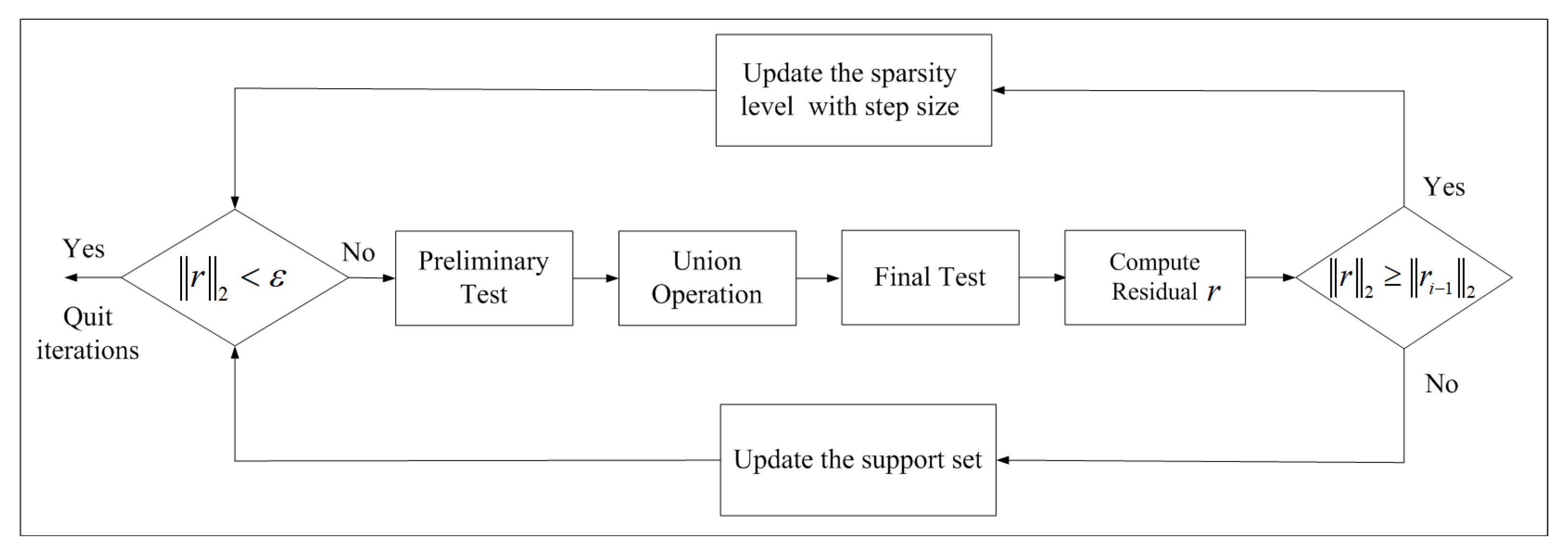
Then, sparsity adaptive matching pursuit (SAMP), which can recover signals without knowing the sparsity level, was proposed by Do et al. [
23]. It alternatively estimates the sparsity level when the residue’s energy increases between two consecutive stages and updates the support set size of the signal using a fixed and small step size. SAMP has apparent advantages when processing one-dimensional sparse signals. However, since one is used as the initial step size, when processing high-dimensional signals, the small step size significantly affects the result and efficiency of reconstruction. To further improve the reconstruction performance, an energy-based adaptive matching pursuit (EAMP) has been proposed [
24]. One limitation of EAMP is that it only focuses on the binary signal reconstruction. Rasha et al. used the structured Wilkinson matrix as the measurement matrix to improve the efficiency of SAMP [
25]. More recently, the improved generalized sparsity adaptive matching pursuit (IGSAMP) algorithm has been proposed. This algorithm uses a nonlinear step size to approximate the sparsity level, and only a small initial step size can be selected. Meanwhile, it requires carefully choosing the parameters without referring to the sensitivity of a large step size [
26].
To improve the reconstruction performance of the sparsity adaptive matching pursuit algorithm and make it less sensitive to the step size, we propose a compositely constrained backtracking matching pursuit (CBMP) algorithm for image reconstruction. The main contributions of this paper are summarized as follows.
- (1)
The restricted isometry property (RIP) is analyzed, and the relationship between observed values and signals is derived and demonstrated.
- (2)
The reconstruction process is divided into three stages, including the large step size stage, small step size stage, and support set update stage. Different step sizes are used in these stages.
- (3)
A backtracking threshold operation is proposed, which adopts a composite strategy and uses dedicated parameters to control the different step sizes in the reconstruction process.
- (4)
The proposed algorithm can achieve satisfactory reconstruction performance and overcome the sensitivity to step size.
3. The Constrained Backtracking Matching Pursuit Algorithm for Image Reconstruction
To overcome the sensitivity to the step size and improve the reconstruction performance of greedy pursuit algorithms, we propose the CBMP algorithm, which introduces restrictions to the backtracking stage, which provides more flexibility as the algorithm gradually approaches the true sparsity level of the unknown signal. The main steps of CBMP are described as follows:
Considering the signal to be reconstructed is a two-dimensional image, the sparsity level is relatively large; the process of sparsity level estimation is divided into large and small step size estimation stages. In the large step size stage, the increment of the step size is . j denotes the stage iteration index. The increment of the sparsity level in the stage of the small step size is fixed and equals the step size of the previous stage.
Due to the advantages of combing information and improving accuracy [
34,
35], a composite strategy is proposed to effectively control the increment of the estimated sparsity level in the two stages. It includes two constraints controlled by parameters
a and
b, which are required in the backtracking threshold operation of CBMP, as described in Algorithm 2. The theoretical support for the composite strategy is clarified as follows:
Theorem 1. Let be a sparse signal and y be a measurement vector. If the measurement matrix Φ satisfies the RIP, then The proof is presented in Appendix A. | Algorithm 2 The proposed CBMP algorithm |
Input: measurement matrix measurement vector step size Initialization: {trivial Initialization}; {initial residue}; {the estimated support set}; {size of the support set (sparsity level)}; {stage index}; i = 1 {}; {union set} Repeat the following steps until the stopping condition holds: 1. Preliminary test: find the matched set indices corresponding to the largest absolute values of that is . 2. Union operation: to broaden the selection space and make candidate list . 3. Final test: to obtain the vector find the matched indices based on the largest absolute values of that is . 4. Compute residual: . 5. Backtracking threshold operation: if and , then shift into the large step size estimation stage: , then shift into 1. if , then shift into the small step size estimation stage: , then shift into 1. Otherwise, shift into the stage that updates the support set based on the current estimated sparsity level: , then shift into 1. Output:{a sparse reconstruction computed by the least squares algorithm}
|
According to Theorem 1, the energy of the original signal x is greater than the square root of one half of that of the measurement vector that is . Different step sizes are used in CBMP. Specifically, the estimated sparsity level is far smaller than the true one at the early stage. Based on this theorem, the energy criterion can be improved by introducing a parameter a to constrain the reconstruction stages.
Inspired by the “four-to-one” practical rule proposed in [
27], the measurement number should be four-times the signal sparsity level for signal reconstruction. In CBMP,
is the union of a new matched set and the estimated support set of the previous iteration.
M is the row number of the measurement matrix. We introduce the “four-to-one” rule to CBMP and use the parameter
b to constrain the estimation stage. The relationship between the parameters
a and
b is analyzed in
Section 4.
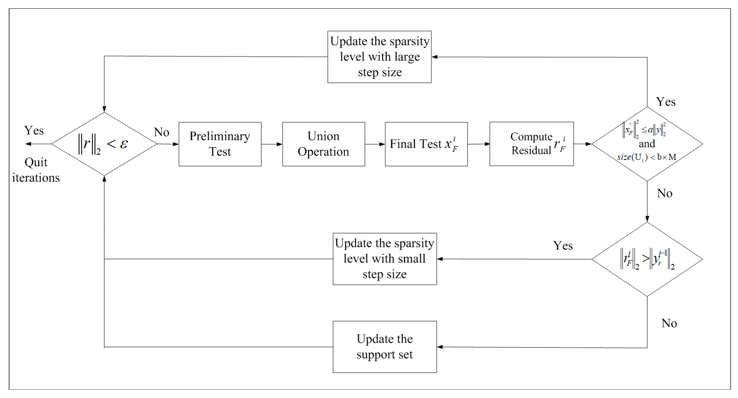
Figure 3 shows the flowchart of the CBMP algorithm. The reconstruction process is divided into the sparsity level update stage and the support set update stage. As for the details, the sparsity level update stage includes both the large and small step size update stages. In the early stage of reconstruction, the estimated sparsity level is far less than the true one, so large step sizes are adopted to estimate the sparsity level. As the iteration goes on, after the threshold condition is satisfied, it enters a small step size stage. The reason why CBMP can achieve better reconstruction performance than SAMP is attributed to its superior capability in handling the wrong indices (atoms). When the current obtained sparsity level is far less than the true one, those false indices can be easily added into the candidate support set. However, these false indices are difficult to eliminate in the later iteration. Therefore, at the beginning of the iteration, a large step size allows those false indices to be filtered out.
4. Experimental Results
Several experiments were conducted to illustrate the performance of the CBMP algorithm. The proposed CBMP was compared with SAMP [
23] and IGSAMP [
26]. The halting condition used by these algorithms was
. For a fair comparison, the same initial step size was used by CBMP, SAMP, and IGSAMP. It should be noted that in SAMP and IGSAMP, the reconstruction results shown in their simulation experiments [
23,
26] are obtained by a small step size (s = 1). In practical applications, when two-dimensional images are stacked into long one-dimensional vectors, the sparsity level in the transform domain is far greater than one. Correspondingly, the step sizes of the proposed algorithm were relatively large. The step sizes used in the experiment were 64, 128, 256, and 512, respectively. Different sampling rates were used to demonstrate the reconstruction performance of CBMP. The wavelet transform was chosen as the sparse basis to represent images. The quality of recovered images was measured by the peak signal-to-noise ratio (PSNR), which is expressed as:
where
,
denotes the original value of the test image at the position
and
denotes the reconstructed value at the position
. The maximum pixel intensity is given as MAX. All images here are expressed using 8 bit intensity values per pixel, so the peak intensity is 255. The experiment configuration is as follows: the CPU was an Intel
® Core™ i5-7200U at 2.50 GHz, and the size of the RAM was 8 GB. The programming language used to perform the experiments was MATLAB. Several experiments were conducted to validate the advantages of CBMP.
According to Theorem 1, . In CBMP, should gradually approach the true one and is much smaller than x at the beginning. Simultaneously, there are two update stages, and then, the threshold parameter a is contracted within . Our experiments demonstrate that the threshold parameters a and b do not distinctively affect the reconstruction performance if the parameter satisfies In CBMP, the support set of the signal obtained by the current iteration is constrained by the parameter a in the step size update stage, while is the union of the estimated support set of the previous iteration and the currently selected support set. Therefore, the relationship between these two parameters is set as . These two parameters play different roles, as a is used after the final test, while b corresponds to the union operation after the preliminary test.
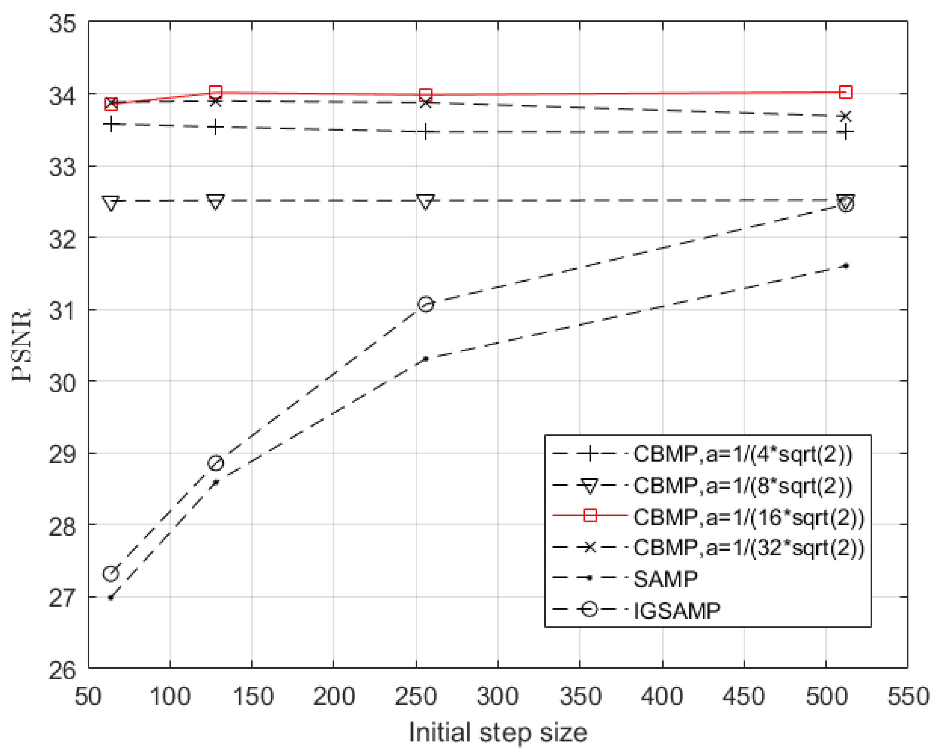
The relationship between the threshold parameters and reconstruction performance is shown in
Figure 4 and
Figure 5. Meanwhile, SAMP and IGSAMP are both tested. Two standard images, “Lena” and “Peppers”, were reconstructed to test the reconstruction performance of different parameter pairs
For a fair comparison, the sampling rate was 0.4, and the same initial step sizes were used. The initial step sizes were chosen from 64 to 512. From
Figure 4, we can see that the reconstruction performance of CBMP with different threshold parameters is better than that of SAMP and IGSAMP. For example, when
, all the PSNR values of CBMP with different initial step sizes are greater than
While the initial step size is
SAMP achieves the maximum PSNR value, which is less than
and IGSAMP offers the maximum PSNR value, which is less than
Therefore, CBMP offers better reconstruction performance than SAMP and IGSAMP. From
Figure 5, it is noticed that if
all the PSNR values of CBMP with different step sizes are greater than
Therefore, the introduction of the threshold operation is necessary for the improvement of greedy pursuit algorithms. At the same time, threshold parameters do not distinctively affect the reconstruction performance if they are satisfied with the constrained condition in CBMP. Meanwhile, the reconstruction performance of CBMP with
is better than the others; thus, this
a value is regarded as the optimal value in the CBMP.
Table 1 and
Table 2 compare CBMP, SAMP, and IGSAMP in terms of the reconstruction performance (PSNR) on the Lena image with different sampling ratios and initial step sizes.
Table 3 and
Table 4 compare CBMP, SAMP, and IGSAMP in terms of the reconstruction performance (PSNR) on the Peppers image with different sampling ratios and initial step sizes.
In
Table 1, when the sampling ratio is 0.3, each PSNR value of the CBMP algorithm is greater than that of SAMP and IGSAMP. For example, with the initial step size of 64, the PSNR value of SAMP and IGSAMP is 25.45 dB and 26.23 dB, respectively, but the PSNR value of CBMP is 32.13 dB.
Table 2 shows the PSNR values of SAMP, IGSAMP, and CBMP with the same sampling ratio of 0.4. Different step sizes are used. The PSNR values of SAMP with different initial step sizes range from 26.99 dB to 31.60 dB. The PSNR values of IGSAMP are increased from 27.32 dB to 32.46 dB. However, the PSNR values of CBMP are greater than those of SAMP and IGSAMP, achieving 33.9675 dB as the average value.
Similarly,
Table 3 shows the PSNR values of the Peppers image by SAMP, IGSAMP, and CBMP when the sampling ratio is 0.3. Each PSNR value of the CBMP algorithm is greater than that of SAMP and IGSAMP.
Table 4 shows the PSNR values of the Peppers image by SAMP, IGSAMP, and CBMP when the sampling ratio is 0.4. Different step sizes are used. For example, as the initial step size is 512, the PSNR value of SAMP and IGSAMP is 30.67 dB and 32.75 dB, respectively, while the PSNR value of CBMP is 32.84 dB.Therefore, CBMP can achieve better reconstruction performance with different sampling ratios and initial step sizes.
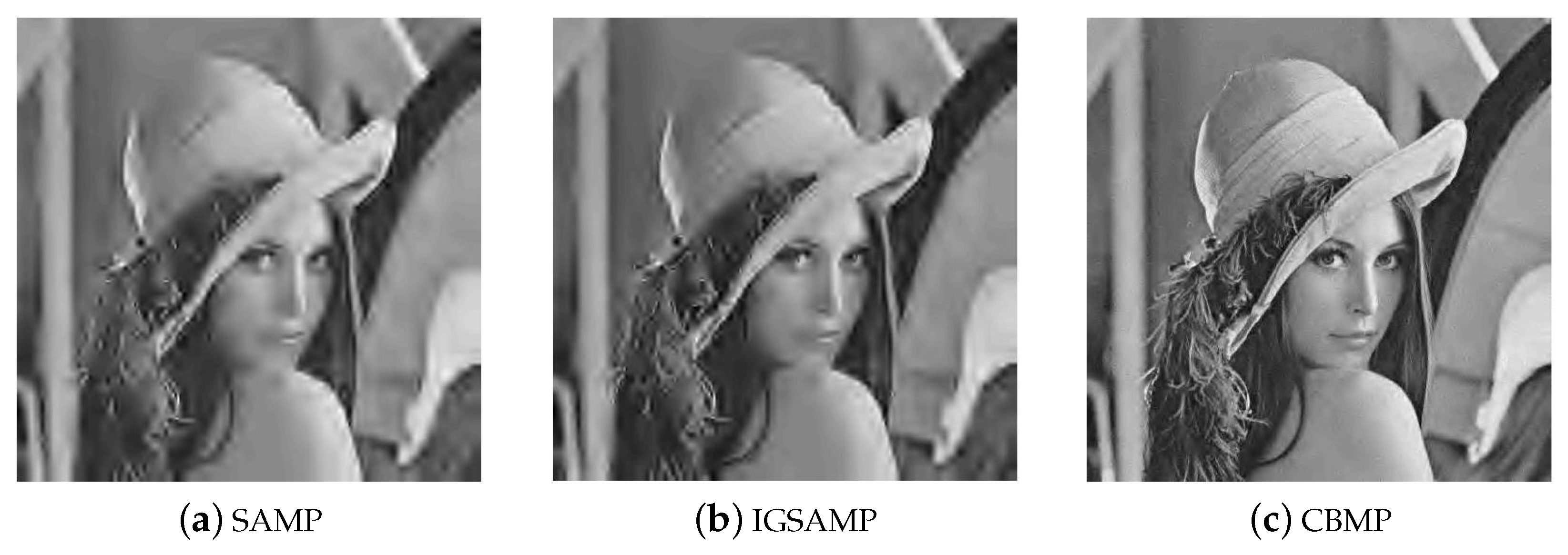
Finally, the reconstructed results of the Lena image using SAMP, IGSAMP, and CBMP are shown in
Figure 6 and
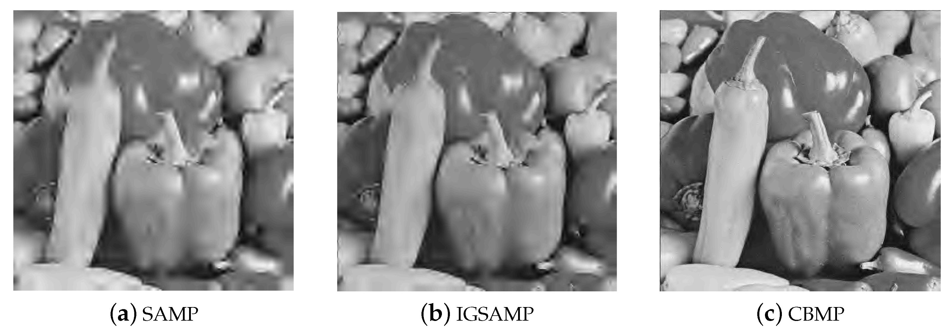
Figure 7. The sampling rate is 0.3; different step sizes are used. The reconstructed results of the Peppers image using SAMP, IGSAMP, and CBMP are shown in
Figure 8 and
Figure 9.
In our test, CBMP outperforms SAMP and IGSAMP in terms of visual effect and PSNR, which is irrelevant to the setup of the initial step size value. At the same time, with different step sizes, the reconstruction performance of CBMP is stable. For example,
Figure 8a and
Figure 9a show different visual reconstruction effects when the initial step size is 64 and 512, individually, and the same conclusion can be made from
Figure 8b and
Figure 9b. It is noted that the visualization effect is not obvious in
Figure 8c and
Figure 9c when the initial step size is 64 and 512, respectively. Therefore, it can be concluded that the CBMP algorithm is relatively insensitive to the step size.


