Weld Metal Microstructure Prediction in Laser Beam Welding of Austenitic Stainless Steel

Featured Application

The proposed modelling of the thermal field allows the evaluation of the fusion zone composition and the solidification mode. With reference to laser beam welding in a single pass of AISI 304L austenitic steel plates, the approach outlines a lean tool for the assessment of the thermal effects on the microstructure resulting from the setup of the main welding parameters, such as the heat source power and welding speed, facilitating the selection of the optimal process conditions, and allowing a proactive welding process control to avoid hot cracking formation.

Abstract

In the present work an approach to weld metal microstructure prediction is proposed, based on an analytical method that allows the evaluation of the thermal fields generated during the laser beam travel on thick plates. Reference is made to AISI 304L austenitic steel as a base material, with the aim to predict the molten zone microstructure and verify the best condition to avoid hot cracking formation, which is a typical issue in austenitic steel welding. The “keyhole” full penetration welding mode, characteristic of high-power laser beam, was simulated considering the phenomenological laws of conduction by the superimposition of a line thermal source along the whole thickness and two point sources located, respectively, on the surface and at the position of the beam focus inside the joint. This model was fitted on the basis of the fusion zone profile, which was experimentally detected on a weld seam obtained by means of a CO₂ laser beam, in a single pass on two squared edged AISI 304L plates, that were butt-positioned. Then the model was applied to evaluate the thermal fields and cooling rates, the fusion zone composition and the solidification mode.

1. Introduction

The tendency toward hot cracking during weld solidification is a serious issue of weldability for austenitic stainless steels, which is influenced by the compositions of base and filler metal and by the level of impurities, such as sulfur and phosphorus [1]. In fact, these elements have a strong tendency to segregate, forming low-melting point eutectics, which are distributed, as a liquid film, along the boundaries of the dendrite grains; then, during the final stage of solidification, they favor the formation of cracks under the force of contraction [2,3].

It is well known that the presence of a small amount of ferrite enhances the resistance to solidification cracking, due to its higher solubility for impurities and the consequent restriction of their partitioning to the interdendritic regions. Therefore, the solidification modes of the austenitic steels (austenitic A, austenitic–ferritic AF, ferritic–austenitic FA) are determinant for the hot cracking phenomenon during cooling from the molten phase [4]. Segregation, and then hot cracking, may occur during the primary austenitic solidification modes (A and AF); conversely, if the austenitic steel solidifies primarily as ferrite-δ (FA), it results less susceptible to hot cracking, due to the higher solubility of the impurities in this phase. The δ/γ interface shows also a better cracking resistance than δ/δ or γ/γ interfaces, because they have higher grain boundary wettability with respect to the eutectic liquid enriched by impurities, as experimentally characterized in [5] and more recently in [6] where the role of the microstructure of the mushy zone is highlighted.

Therefore, the metallurgical features that accompany the transition between AF and FA solidification modes are crucial to establishing the material susceptibility to hot cracking, considering also other issues, such as sensitizing to intergranular corrosion and loss of toughness, due to carbide precipitation and to the formation of embrittling phases [7]. In this respect the ability to predict microstructures and properties of the austenitic stainless steels, according to their composition, has been the topic of many studies. Starting from the historical works of Schaeffler and DeLong, David et al. [8] investigated the effects of cooling rate, Siewert et al. [9] proposed a new ferrite diagram (WRC 1988) that shows, in the austenite/ferrite zone, the ferrite percentages, or ferrite number (FN); then the diagram was modified by Kotecki and Siewert [10] by the inclusion of the solidification mode boundaries (WRC 1992), obtaining a very useful tool to predict weld microstructure on the base of the grade of dilution. This kind of diagram is still attractive for phase evaluations based on the fused zone composition, especially in the case of dissimilar welds [11,12]. Other than composition, cooling rate [13] is a non-negligible parameter in determining the solidification modalities, which in turn results from the welding conditions.

In recent years, numerous studies have been developed to simulate, by the finite element method (FEM), the thermal fields generated during welding: for a review on these numerical methods, see the articles by Rong et al. [14] and Marques et al. [15]). In particular, Sun et al. carried out a work to evaluate the dilution grade in multi pass arc welding and predict the final microstructure of the weld [16]; more recently, Kick [17] calibrated the heat source by selecting the finite element mesh in such a way that the calculated shape of the molten pool corresponded to that from real tests.

In any case, these numerical simulations require increasing computing capacity and time, according to the degree of accuracy of the mesh into which the joint is subdivided [18], and needs to be validated by experimental measurements which, by their nature, are specific of the welding conditions considered [19].

A less complex approach, from the point of view of the thermal field calculation, is given by the phenomenological laws of the heat conduction, which are based on the integration of the Fick’s second law and consist in analytical solutions developed starting from the well-known equation proposed by Rosenthal [20]. Considering a reference system (x,y,z) whose origin is fixed to the thermal source that moves along the welding axis x with speed v (m/s), in the case of a point heat source Q_P (W) the temperature T(x,y,z) in a generic point is given by the following equation:

$$\mathrm{T}\left(\mathrm{x},\mathrm{y},\mathrm{z}\right){=\mathrm{T}}_0+\frac{{\mathrm{Q}}_{\mathrm{P}}}{{\mathrm{c} \mathsf{\pi } \mathrm{k} \mathrm{r}}_{\mathrm{P}}}{\mathrm{e}}^{-\frac{\mathrm{v}}{2\mathsf{\alpha }}\left({\mathrm{r}}_{\mathrm{P}}+\mathrm{x}\right)},$$

(1)

where T₀ is the initial temperature, c a numeric coefficient, k (W/mK) the thermal conductivity, α (m²/s) the diffusivity, r_P (m) the radial distance from the point source:

$${\mathrm{r}}_{\mathrm{P}}=\sqrt{{\mathrm{x}}^2{+\mathrm{y}}^2+{\left(\mathrm{z}-{\mathrm{z}}_{\mathrm{P}}\right)}^2},$$

(2)

where z_P is the depth of the mobile source respect to the axes’ origin, which is located on the body surface.

The numeric coefficient in the denominator of Equation (1) is c = 2 when z_P = 0 (point source on the body surface) and c = 4 when z_P > 0 (point source inside the body).

In the case of a mobile source uniformly distributed on a line along the body thickness (z axis), Rosenthal gives the following equation for the temperature fields in the plane xy [20]:

$$\mathrm{T}\left(\mathrm{x},\mathrm{y}\right)={\mathrm{T}}_0+\frac{{\mathrm{Q}}_{\mathrm{L}}}{2 \mathsf{\pi } \mathrm{k}}{\mathrm{e}}^{-\frac{\mathrm{v}}{2\mathsf{\alpha }}\mathrm{x}}{\mathrm{K}}_0\left(\frac{{\mathrm{v} \mathrm{r}}_{\mathrm{L}}}{2\mathsf{\alpha }}\right),$$

(3)

where Q_L (W/m) is the power per unit of the source length, K₀ the modified Bessel function of the second kind of order zero, r_L (m) the radial distance from the source in the plane xy:

$${\mathrm{r}}_{\mathrm{L}}=\sqrt{{\mathrm{x}}^2{+\mathrm{y}}^2}.$$

(4)

As was exposed in a recent review [21], subsequent works, starting from those of Carslaw and Jaeger [22] and Ashby and Easterling [23], have offered further simulations of the temperature fields generated by the advancement of mobile heat sources of various geometries with surface energy distributions.

However, in the case of high-power laser beam welding, a modelling based only on heat conduction does not take into account the complex fluid dynamics phenomena inside the keyhole, which give rise to thermal distributions that are very difficult to simulate analytically. So, in order to compensate for the simplification inherent in the modelling carried out according to the laws of heat conduction, in this work the authors consider an experimentally-fitted multipoint-line system of the thermal sources, which was proposed in a previous paper [24]. The actual heat input generated by the “keyhole” and its effects on the melt pool and on the weld cross sections are simulated through the adoption of parameters which define the sources layout and the power distribution between them. Due to such peculiarities the fitted model is suitable to analyze in detail the overall thermal field due to a moving heat source that simulates the laser beam welding effects, also focusing on the temperature profiles, as time varies, in fixed detection points of the workpiece.

In this work the analytical model was further implemented by developing the derivatives of the temperature–time curves with the aim of evaluating the cooling rate, which is a crucial parameter for the weld microstructure. So, the model was applied to a laser beam butt-welding, with a single pass, of austenitic stainless-steel plates with the interposition of filler material in the form of thin sheets. The keyhole effect was modelled by a heat sources system constituted by a line source along the entire thickness and two point sources located, respectively, on the surface and inside the joint, at the focus point of the laser beam. The parameters of the source system were set in order to obtain the best fit between the analytical profile of the fused zone (FZ) and the one detected experimentally. The resulting thermal field was used to calculate the FZ boundaries and to simulate the cooling rate distribution, in order to predict the weld composition and microstructure, with the aim to define the solidification mode and susceptibility to hot cracking.

2. Materials and Methods

2.1. Welding Process and Materials

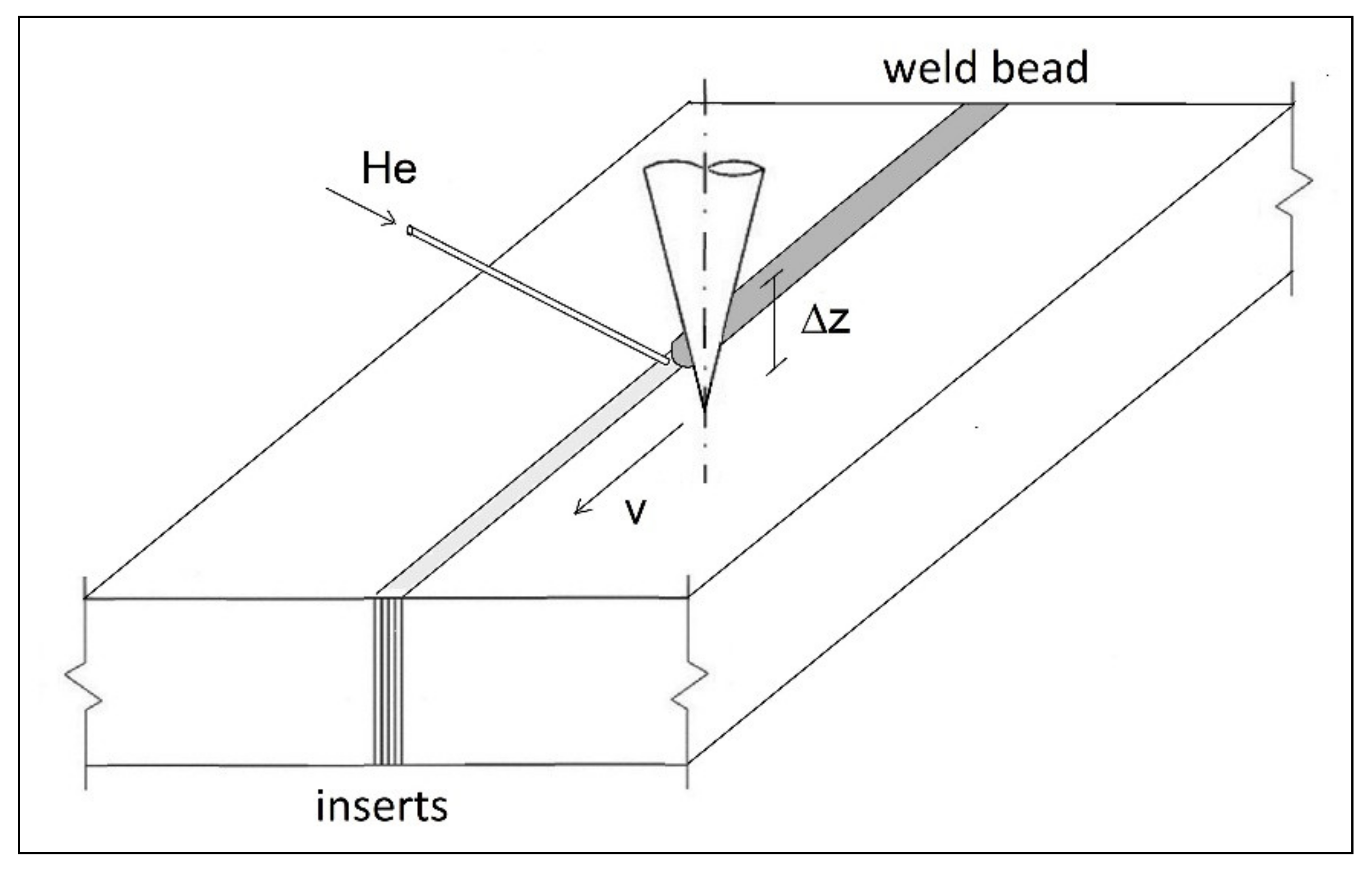
A CO₂ gas laser beam apparatus UT (United Technologies, East Hartford, CT, USA) with a maximum yield power of 25 kW, operating in robotic mode, was used to butt-weld two stainless steel plates in a flat position (Figure 1). Welding was carried out in a single pass. The plates (each one with size 1000 × 1000 mm, thickness of 10 mm), were made of AISI 304L austenitic steel as base material (BM), which was selected for its good weldability due to the reduced carbon content [24]. They were prepared with square edges, no gap, and filler material (FM) interposed in the form of four consumable inserts (each one being a sheet with size 1000 × 10 mm, thickness 0.4 mm), initially fixed by gas tungsten arc tack-welding.

The optical device consisted of a paraboloid mirror with a focal length of 682 mm. By means of a diagnostic system, the operating parameters were checked before welding, evaluating the laser beam quality, depending on degree of focusing, diameter and position of the focus, which was located inside the plates at a distance Δz from their upper surface (

Table 1. Welding parameters.

Laser Beam Power P (kW)	Welding Speed v (m/min)	Focus Diameter (mm)	Focus Position Δz (mm)	Helium Flow Rate (L/min)	Insert Width (mm)
14	1.2	0.5	5.5	20	1.6 (4 sheets, each width 0.4 mm)

).

At the experimented power level, the incident beam energy is so high that the portion of irradiated material melts and vaporizes, forming a capillary cavity (keyhole), surrounded by molten metal. At high temperatures, a part of the vapor ionizes forming plasma, which is harmful because it absorbs energy and attenuates the laser beam effects. The control of plasma was performed by a transverse helium flow, through a nozzle with an internal diameter of 4 mm, directed above the interaction zone of the laser beam with the molten bath. The use of helium, which is technically preferable to argon although more expensive, is justified by a greater resistance offered to ionization.

The compositions of FM and BM are shown in

Table 2. Composition of the base metal and the filler (% by weight).

	C	Mn	Si	P	S	Ni	Cr	Mo	Fe
AISI 304L	0.018	1.15	0.41	0.025	0.001	10.1	18.4	-	Bal.
AWS 309L 1	0.010	1.65	0.33	0.020	0.010	12.4	24.5	0.47	Bal.
AWS 308L 2	0.025	1.40	0.30	0.030	0.030	10.0	20.0	-	Bal.

¹ Filler material (FM) utilized for the experimental welding trials. ² FM considered for simulation.

. Instead of AWS 308 L (considered commonly for welding AISI 304L stainless steel [25]), the inserts used were made of AWS 309 L, in order to diversify the composition of the FZ with respect to that of the BM and compare the levels of Ni and Cr detected experimentally in the joint with those obtained by applying the analytical model. The welded bead was subjected to visual inspections for a quality check and to macrographic observations by a stereo microscope Leica MZ 16 1FA (Leica Microsystem, Milan, Italy) on some cross sections cut at regular intervals along the weld bead, in any case far from the ends. The cross-section surface was prepared by mechanical grinding with abrasive paper (gradation from 180 to 2400), polishing by a velvet cloth with an aqueous suspension of 0.5 µm Al₂O₃ and etching through the Glyceregia reagent (16% HNO₃, 42% HCl, 42% glycerol). The FZ microstructure was characterized by an optical microscope Olimpus G71 (Microscope System Limited, Glascow, UK). Finally, the Ni and Cr contents in the FZ were detected performing energy dispersive X-ray spectroscopy EDS measurements on the welded section by means of a JEOL JSM-7610F apparatus (JEOL Ltd., Tokyo, Japan). The EDS measurements were performed in automatic mode, with no less than 100,000 counts in order to have a precision of 1% with a confidence level of 99%. As for the accuracy, the detector error can be estimated by the relative deviation from the expected value, that is the relative error ε between the measured composition C and the true value C_true (i.e., the concentration of the elements known from an independent analysis): ε = (C − C_true)/C_true. In [26] Newbury and Ritchie determined for an austenitic stainless steel (Fe = 71%, Cr = 18.3%, Ni = 10.7%,), the following values for the relative error of the composition measured by a JEOL apparatus: ε(Fe) = 0.0008, ε(Cr) = 0.0087, ε(Ni) = 0.02.

This specific welding procedure, already tested in [27], was chosen because, in addition to being easy to use, it ensures great tolerance with respect to any geometric imperfections in the preparation of the edges and/or errors in the alignment of the beam; moreover, with a correct number of inserts, it allows the avoidance of the risk of incomplete fusion more easily than using filler wire. By this way, it is also possible to obtain joints with a limited presence of defects and an easier control of the degree of dilution [28].

2.2. Thermal Field Modelling and Analysis

An experimentally-fitted multipoint-line heat sources approach previously presented [24] was used for thermal field modelling. This approach is based on the configuration and fitting of a generalized conductivity-based model, aimed to set up the system of types (1) and (3) sources, able to produce the same thermal effect of the actual interaction between the laser beam and the workpiece, without evaluating the complex energy-transfer processes that characterize keyhole mode laser welding. This effect is represented by the shape and boundaries of the weld bead on the plane orthogonal to the direction of source movement. The generalized model can be adapted to the specific case to be analyzed, on the basis of the geometrical features of the experimentally detected bead cross-section.

By varying the configuration of the model, it is possible to simulate the thermal sources system capable of determining the laser welding beads of the most common shapes, from those typical of deep penetration laser welding, to those characterized by low penetration and parabolic cross-section beads. After the setup of the most suitable combination of heat sources, the multi-source model is defined in detail by fitting, on the shape of the bead cross-section experimentally detected, the parameters that characterize the geometric layout and strength of the sources: the length of the line source and the location depth of the point sources (z_L, z_P1, …, z_Pi, …), which define the layout of the model; the distribution coefficients (γ_L, γ_P1, …, γ_Pi, …) of the laser’s thermal power absorbed by the keyhole, which define the strength distribution among the sources.

In the case under consideration, the thermal analysis was carried out by an analytic model based on the superimposition of two point sources and one line source, whose thermal fields, according to the conductivity-based modelling previously introduced, are expressed by Equations (1) and (3):

$$\mathrm{T}\left(\mathrm{x},\mathrm{y},\mathrm{z}\right)={\mathrm{T}}_0+{\displaystyle {\sum }_{\mathrm{i}=1}^2\frac{{\mathrm{Q}}_{\mathrm{Pi}}}{{\mathrm{c}}_{\mathrm{i}}{\mathsf{\pi }\mathrm{kr}}_{\mathrm{Pi}}}{\mathrm{e}}^{-\frac{\mathrm{v}}{2\mathsf{\alpha }}\left({\mathrm{r}}_{\mathrm{Pi}}+\mathrm{x}\right)}}+\frac{{\mathrm{Q}}_{\mathrm{L}}}{2\mathsf{\pi }\mathrm{k}}{\mathrm{e}}^{-\frac{\mathrm{v}}{2\mathsf{\alpha }}\mathrm{x}}{\mathrm{K}}_0\left(\frac{{\mathrm{vr}}_{\mathrm{L}}}{2\mathsf{\alpha }}\right),$$

(5)

where T₀ is assumed equal to the room temperature (293 K).

To simulate the full penetration welding and the keyhole effect, reproducing the experimental profile of the molten area in the best possible way, the thermal sources were located as follows:

• First point source on the external surface, at the laser beam side (z_P1 = 0 mm);
• Second point source inside the bead where the beam is focused (z_P2 = Δz = 5.5 mm);
• Line source along the whole bead thickness (z_L = 10 mm).

This choice was made according to the morphology of the FZ profile in the welded section: the line source contributes to the formation of a regular shape of the FZ along the entire thickness, while the point sources give rise to the convexities that characterize the experimental profile, respectively, near the surface exposed to the laser beam and inside the joint, where the beam is focused.

Once the model layout was defined, the sources’ strength parameters γ_L and γ_Pi were introduced in order to distribute the overall power of the laser beam between the line and the two point sources. Of course, the sum of these partition coefficients of the thermal power must respect the condition: γ_L + γ_P1 + γ_P2 = 1.

Being P = 14 kW, the net power carried by the laser beam, the fraction absorbed by the plates can be expressed by introducing the coefficient η < 1, in order to exclude the fraction absorbed by the plasma and dispersed in the environment. Therefore, the following expressions of the power delivered by each source are defined by the following expressions:

$${\mathrm{Q}}_{\mathrm{Pi}}={\mathsf{\gamma }}_{\mathrm{Pi}}\mathsf{\eta }\mathrm{P}\hspace{1em}\hspace{1em}\hspace{1em}{\mathrm{Q}}_{\mathrm{L}}={\mathsf{\gamma }}_{\mathrm{L}}\mathsf{\eta }\mathrm{P}/{\mathrm{z}}_{\mathrm{L}},$$

(6)

under the condition of balancing the total power input:

$$\mathsf{\eta }\mathrm{P}={\displaystyle {\sum }_{\mathrm{i}=1}^2{\mathrm{Q}}_{\mathrm{Pi}}}+{\mathrm{Q}}_{\mathrm{L}}{\mathrm{z}}_{\mathrm{L}}.$$

(7)

The absorption coefficient η in Equations (6) and (7), and the sources’ strength distribution parameters γ_Pi and γ_L, are variables to be determined numerically to allow the best fitting of the analytical profile on the experimental FZ boundaries.

The construction of a 3D model of the FZ was achieved by applying Equation (5) to obtain the isothermal curves at the solidus temperature (T_S = 1673 K) on horizontal planes at different values of z. For the thermophysical parameters of the AISI 304L steel, constant values at an intermediate temperature equal to 700 °C were assumed [29]: density ρ = 782 kg/m³, thermal conductivity k = 25 W/(mK), diffusivity α = 5.42 × 10⁻⁶ m²/s.

Equation (5) allows the expression of the thermal field of the two point and line sources model in each point (x,y,z) according to the reference system fixed on the heat source moving on the surface of the workpiece. To analyze the temperature cycles in a fixed detection point, as time varies, i.e., as the distance of the mobile sources from the detection point varies during their movement, the following coordinate transformation must be operated in Equation (5):

$$\mathrm{x}\to \mathsf{\xi }=\mathrm{x}-\mathrm{vt},$$

(8)

where v is the moving speed along the x axis, and t is the time.

By means of this transformation, a fixed point on the workpiece, with respect to the mobile reference system xyz, is identified by the coordinates (ξ,y,z).

The model was further implemented to determine the rate of thermal variation in (ξ,y,z) fixed points of the workpiece, deriving with respect to time Equation (5) to which the transformation x→ξ is applied:

$$\begin{gathered} \frac{\partial \mathrm{T}\left(\mathsf{\xi },\mathrm{y},\mathrm{z}\right)}{\partial \mathrm{t}}={\displaystyle {\sum }_{\mathrm{i}=1}^2\left[\frac{{\mathrm{a}\prime }_{\mathrm{i}}{\mathrm{v} \mathsf{\xi } \mathrm{e}}^{-\mathrm{b} \left({\mathrm{r}}_{\mathrm{Pi}}+\mathsf{\xi }\right)}}{{\mathrm{r}}_{\mathrm{Pi}}^3}-\frac{{\mathrm{a}\prime }_{\mathrm{i}}\mathrm{b} \left(-\frac{\mathrm{v} \mathsf{\xi }}{{\mathrm{r}}_{\mathrm{Pi}}}-\mathrm{v}\right){ \mathrm{e}}^{-\mathrm{b} \left({\mathrm{r}}_{\mathrm{Pi}}+\mathsf{\xi }\right)}}{{\mathrm{r}}_{\mathrm{Pi}}}\right]}+ \\ \left[{\mathrm{a}″\mathrm{b} \mathrm{v} \mathrm{e}}^{-\mathrm{b}\mathsf{\xi }}{ \mathrm{K}}_0\left({ \mathrm{b} \mathrm{r}}_{\mathrm{L}}\right) +\frac{{\mathrm{a}″\mathrm{b} \mathrm{v}\mathsf{\xi } \mathrm{e}}^{-\mathrm{b}\mathsf{\xi }}{ \mathrm{K}}_1\left({ \mathrm{b} \mathrm{r}}_{\mathrm{L}}\right)}{{\mathrm{r}}_{\mathrm{L}}}\right], \end{gathered}$$

(9)

where a′_i = Q_Pi/c_iπk, a″ = Q_L/2πk, b = v/2α, r_Pi and r_L are expressed by Equations (2) and (4) where transformation x→ξ is applied, K₀ and K₁ are the modified Bessel function of the second kind of order zero and one. This equation allows the calculation of the heating and cooling rates at each point (ξ,y,z), as the heat sources approach it and move away along the x direction, respectively.

3. Results

3.1. Weld Inspection

Upon visual inspection, carried out through a reader lens equipped with led light without taking photos, the welded bead resulted free from cracks and other macroscopic defects. Macrographic observations of the cross-section show a full penetration of the FZ along the whole plates thickness (Figure 2a): the FZ has a regular shape, with a width of about 2 mm, which becomes slightly wider near the external surface at the laser beam side and shows a certain enlargement in correspondence to the focus position. From a metallographic point of view, the FZ is characterized by a homogeneous dendritic structure, with the presence of residual ferrite in the austenitic matrix (Figure 2b). From the image analysis, performed by means of ImageJ software (US National Institutes of Health) on the four boxes defined in Figure 2b, thus obtaining the elaborations shown in Figure 2c, resulted a volumetric percentage mean value of ferrite equal to 15.65% with a standard deviation equal to 1.94.

Due to the choice of the AWS 309L as filler, the FZ is more alloyed than the base metal: in fact, the EDS measurements gave Cr and Ni contents, respectively, equal to 22.7% and 12.0% [27].

3.2. Weld Zone Modelling

Figure 3 shows the 3D modelling of the melt pool together with the comparison between the calculated FZ profile and the one detected experimentally in the cross-section plane. The calculated profile was obtained by projecting the maximum contour of the 3D model of the molten pool onto the yz plane (Figure 3a). In this way, the imprint of the maximum width of the FZ on the cross section of the joint was obtained. The fitting with the experimental profile was optimized by minimizing the sum of the squared distances along the y axis, between the experimental and the theoretically calculated profiles, at four different depths along the z axis, drawn by dashed lines in Figure 3b. The optimization was performed by the evolutionary solving tool implemented in Excel, obtaining the convergence to a stable solution that closely approximates the experimental profile. Both calculated and experimental profiles in Figure 3b include the grey rectangle, which indicates the area occupied by the four consumable inserts, demonstrating that thermal input is sufficient for their complete fusion together with a part of the base material.

As a result of this procedure, the distribution parameters of the beam power (γ_L = 0.81, γ_P1 = 0.10, γ_P2 = 0.09) and the absorption coefficient (η = 0.51) were obtained. In particular, the latter value is included within the range η = 0.50-0.80, which was defined on the basis of the minimum and maximum value available in the literature for laser beam welding of steels according to the “keyhole mode” [30,31]. A further study quoted in the literature [32] presents a calculation model for the absorption coefficient that allows the estimation η = 0.55. However, the portion of energy that actually enters the keyhole is considered and that the wings of the incident radiation distribution are not so intense as to melt the material, in the case of steels [30] a further reduction in the laser beam power, around 6–10%, can be assumed, obtaining for η a range of values between 0.49 and 0.52. This observation further validates the fitting of the calculated profile to the experimental one.

Once the model has been fitted, various simulations to evaluate the effects of the mobile heating source can be performed. In Figure 4a the isotherms in the plane xy at z = 5 mm are drawn for three significant temperatures: a 1400 °C solidus temperature, 500 °C lower limit and 850 °C upper limit of temperature for carbide precipitation. The temperature–time curves, obtained by means of x→ξ transformation (8), are shown in Figure 4b at different distances y from the welding axis, starting from y = 1.37 mm, i.e., the FZ boundary.

The rates of thermal variation in fixed points of the workpiece, which are the results of the derivation operations on the temperature–time curves, were calculated by Equation (9), and are shown in the Figure 5: it can be observed that within the FZ, at y = 0.2 mm, the cooling rate is very high, reaching a maximum value of 6 × 10⁴ K/s, while its value is reduced to 1 × 10³ K/s at the FZ boundary (y = 1.37 mm). The results of thermal rates calculation by Equation (9) are reported starting from y = 0.2 mm because, for lower values of y, that means greater proximity to the welding line, the Rosenthal-type equations lose reliability, being based on the incident point source hypothesis, that leads to infinite temperature at the sources (y = 0) [20].

4. Discussion

The isotherms in Figure 4a give an indication of the width of the FZ and the zone heated in the sensitizing range of temperature. First of all, the analytical model was considered to evaluate if steel become sensitized: so, the intersections of the temperature–time curves with the horizontal lines, which define the boundaries of the sensitizing interval, allow the calculation of the permanence time in the range 500–850 °C (Figure 4b). In the case under examination, it can be concluded that, due to the short time (about 4 s), this kind of deterioration has to be excluded [1].

The filler material composition and the degree of dilution are decisive for the properties of the joint. Considering the area occupied in the cross-section by the experimental filler inserts made of AWS 309L (A_FM = 16 mm²) and the calculated area of the FZ (A_FZ), the weld bead composition can be obtained by carrying out a weighted average of the BM and FM compositions, using as weights, respectively, 1-A_FM/A_FZ and A_FM/A_FZ. The results are reported in

Table 3. FZ composition, cooling rate, ferrite volume (insert made of AWS 309L).

		Calculated Compositions (% weight)						CR (K/s)	Ferrite (% vol.)			SM
AFZ (mm2)	AFM/AFZ	C	Ni	Cr	Mo	Nieq	Creq		Meas. value	Ref. [10]	Ref. [8]	Ref. [10]
25.9	0.62	0.013	11.5	22.2	0.29	12.0	22.5	6 × 104	15.65	21.0	12.0	FA

, together with the equivalent compositions, calculated according to the WRC-1992 diagram [10]:

$${\mathrm{Ni}}_{\mathrm{eq}}=\%\mathrm{Ni}+35 \%\mathrm{C}\hspace{1em}\hspace{1em}\hspace{1em}{\mathrm{Cr}}_{\mathrm{eq}}=\%\mathrm{Cr}+\%\mathrm{Mo},$$

(10)

Other than composition, cooling rate (CR) is a crucible parameter to predict both the solidification mode (SM) and fused zone microstructure [33]. Thus, in the same table the following parameters are also shown: the maximum value of CR calculated inside the FZ (at y = 0.2 mm) by means of Equation (9), percentage of the residual ferrite-δ, respectively, according to the WRC-1992 [10] and to the work of David et al. [4], solidification mode (SM) determined through use of the WRC-1992.

It can be observed that the calculated contents of Ni_eq (12.0%) and Cr_eq (22.5), agree with the values measured experimentally by EDS, which are, respectively, equal to 12.0% and 22.7% (mean values with standard deviations, respectively, equal 0.39 and 0.23, obtained from performing 10 measurements).

The content of ferrite in the FZ (15.65%), detected experimentally by image analysis of the micrograph (Section 3.1), is within the range of the values quoted in [8,10]. In particular, it is lower than the FN value, equal to 21%, which can be derived from the WRC-1992 diagram for Cr_eq = 22.5 and Ni_eq = 12.00. Moreover, this composition falls in the field of the FA solidification mode. Nevertheless, the WRC-1992 diagram does not give any indication about the cooling rates involved, which, however, could have a significant effect. In this respect, the maximum cooling rate calculated by us in the FZ is near to the value 6 × 10⁴ K/s, which is quoted in the experimental work [8] for a solidification mode FA and a residual ferrite content equal to 12%, closer to our percentage than that in [10].

The austenitic steels, when the ratio Cr_eq/Ni_eq is in the range 1.5–2.0, solidify as ferrite-δ. Then, if the cooling rate is sufficiently low, it is transformed into austenite (FA mode), according to the following sequence of transformations [34]:

$$\mathrm{L}\to \mathrm{L}+\mathsf{\delta }\to \mathrm{L}+\mathsf{\delta }+\mathsf{\gamma }\to \mathsf{\delta }+\mathsf{\gamma }\to \mathsf{\gamma },$$

(11)

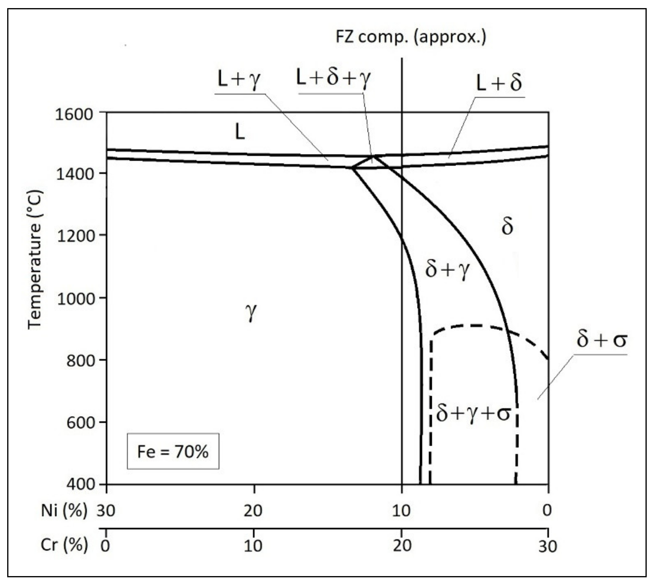
At the later stages of solidification, some secondary austenite solidification in the interdendritic regions may take place. In any case, during the subsequent cooling, the ferrite stability decreases with respect to austenite, resulting in the diffusion-controlled transformation of ferrite into austenite. If there is enough time to allow this process to go towards completion, the final ferrite content at room temperature reaches the equilibrium value, which is given by the ternary phase diagram Fe-Cr-Ni (Figure 6).

As mentioned above, the WRC-1992 diagram does not take into account the effect of cooling rate values, neglecting the role of this parameter. In the FA mode, the percentage of residual ferrite increases with increasing cooling rate, because the δ→γ transformation has less time to occur, and so the δ phase becomes frozen at low temperature. In the case of a very fast cooling rate, the FA mode is altered and the austenitic steels, that normally solidify as primary ferrite, may solidify as primary austenite instead; however, even if the solidification mode changes to primary austenite, some secondary ferrite can be observed at room temperature. For 309A steel considered in [35] (having a composition similar to that calculated for the FZ in Table 3), the switch from the primary ferrite to primary austenite solidification mode takes place at cooling rates greater than 10⁶ K/s [36], which can be excluded in the case examined here.

Solidification as primary ferrite (FA mode) has been shown to ensure better resistance to weld solidification cracking than the other modes. In general, austenitic stainless steels tend to be less susceptible to solidification cracking if the primary solidification phase is ferrite-δ. The main reason is the presence of ferrite–austenite boundaries at the end of solidification, which resists wetting by liquid films and presents a tortuous path (see Figure 7), along which cracks have more difficulty propagating than if they were straight and smooth.

However, the presence of too much ferrite may give adverse effects, because grain can be selectively attacked by certain corrosive media; moreover, at operating temperatures in the range of carbide precipitation, ferrite transforms into the brittle σ phase. Therefore, the FZ composition was calculated again by hypothesizing the inserts made of AWS 308L (

Table 4. FZ composition, cooling rate, ferrite volume (hypothesizing AWS 308L inserts).

		Calculated Compositions (% Weight)						CR (K/s)	Ferrite (% vol.)		SM
AFZ (mm2)	AFM/AFZ	C	Ni	Cr	Mo	Nieq	Creq		Ref. [6]	Ref. [4]	Ref. [6]
25.9	0.62	0.022	10.0	19.4	-	10.8	19.4	6 × 104	10.0	13.5	FA

). In this case lower values of Cr_eq and Ni_eq were obtained, to which corresponds FN = 10 in the WRC-1992 diagram.

5. Conclusions

A parameterized model, based on the assumption of a virtual heat sources system consisting of two point sources and a line source, was used to analytically define the thermal field due to high power laser welding, and its derivative with respect to time. It was applied to simulate the thermal cycles in fixed points of the workpiece and the cooling rates due to full penetration laser beam butt-welding of AISI 304L plates with consumable insertion of AWS 309 L as filler material, with the aim to predict weld composition and microstructure.

The compositions of Ni and Cr, calculated in the fused zone, agree with the values measured experimentally. The calculated composition allowed the prediction of microstructure and solidification modes through the WRC-1992 diagram, which consists of residual ferrite in an austenitic matrix as demonstrated by the metallographic observations and is a microstructure effective at reducing the risks of hot cracking. The weld microstructure prediction is confirmed by the results of cooling rate calculation, which agree with the data presented in the literature for the solidification mode as primary ferrite.

To obtain a lesser percentage of ferrite, more suitable for a good resistance to corrosion, the use of less alloyed inserts, made of AISI 308L, is necessary, as verified by simulation.