Featured Application
This work demonstrates the feasibility of using wireless networks with Wi-Fi technology in the deployment of sensor networks for precision agriculture.
Abstract
The application of deficit irrigation techniques is essential in arid or semi-arid areas of the southeast of Spain, where water is a scarce and very costly resource. However, to apply these techniques, it is necessary to carry out preliminary tests on the specific crop in order to develop the models that allow the optimization of water use while achieving acceptable yields. The system proposed in this article demonstrates the feasibility of using wireless technologies available in most facilities (Wireless Fidelity) to deploy a high-density network of nodes with a variety of heterogeneous sensors to collect data from the soil, plant, and atmosphere. The data are sent and stored in a cloud server for real-time visualization from any mobile device and further analysis. The nodes have been developed using low-cost processors and are equipped with batteries and solar panels, allowing their autonomy to be virtually unlimited, as shown by the consumption studies and tests carried out.
1. Introduction
In arid and semi-arid zones, such as the southeast of Spain, the agriculture yield is conditioned by limiting factors, the main one being the available irrigation water. Regulated deficit irrigation (RDI) techniques allow controlling the water applied to the crop in critical and non-critical phenological stages, determining periods where the crop can be irrigated with much less water. Therefore, these techniques have been widely used in these areas where water is a scarce resource [1,2,3]. However, the application of RDI strategies is conditioned by crop and climatic conditions. The development of irrigation models specifically designed for a crop would allow the application of RDI for water optimization purposes. In order to develop these models, it is necessary to carry out several comparative tests on different areas of the same crop, where the conditions of the applied RDI are modified. By studying the production and soil and plant water relations on trees subjected to the different treatments, it is possible to determine the most appropriate models for optimal irrigation management. In order to establish these RDI models, sensors that report on the state of the soil, plant and atmosphere are required. In addition, to achieve sufficient precision, it is important to have several repetitions of the measurements deploying different deficit irrigation regimes to obtain relations among the agronomic results and the water stress indicators studied [4,5,6].
Sensor networks are widely used when a high density of instrumentation is required on test plots. In the particular case of wireless sensor networks (WSN), their usefulness has been demonstrated in different papers [7,8,9,10], where the absence of wiring has resulted in a very important improvement in terms of installation flexibility and time savings in installation and maintenance. Several protocols have been described in the bibliography for the deployment of WSN in precision agriculture (PA) [11,12]. Zigbee is one of the most commonly used technologies in recent years with positive results [13,14,15,16,17,18], although it is claimed that ZigBee communication has the problem of short distance, complicated networking and high communication frequency [19]. From the experience of our research group in previous installations, in which we deployed WSNs with Zigbee nodes [20,21,22,23], we found significant drawbacks such as the high maintenance required by the nodes, the difficulty of programming the Zigbee stack, the high price of the software licenses and the limited availability of microcontrollers that supported this stack. Some authors such as [11], who conducted a comprehensive review of WSN technologies and their applications in PA, claim that the most suitable technology for this type of applications is narrowband internet of things (NB-IoT). A well-known example is long-range radio (LoRa), which allows very low energy consumption and long life (i.e., 10 years with battery), low cost, wide coverage and large networks (52,000 devices/channel/cell). This is why LoRa is being used extensively in IoT applications in all fields, including PA [19,24,25,26,27,28,29,30,31,32]. However, there are numerous WSN deployments in PA that use 802.11 wireless fidelity (Wi-Fi) [18,33,34,35,36,37,38]. It is important to highlight that the suitability of each technology in terms of range, robustness and, above all, in terms of instrumentation capacity, must be analyzed and studied to use it properly. Wi-Fi networks have also been used previously in other disciplines such as post-harvest for monitoring perishable products in transport and conservation [39].
The sensor network described in this article aims to support agronomic trials to relate criteria of deficit irrigation in almond trees with measured values of soil-plant-atmosphere. To this end, it is necessary to study different deficit irrigation treatments. Due to the size of the plot, the number of trees and parameters to measure, a large and reliable network infrastructure was needed. WSN was selected as the best option for this study, since cabling would be very expensive and unfeasible in practice (due to the need of ducts and ditches, problems with animals, soil moisture...) and a Wi-Fi network was already available at the farm. In particular, using Wi-Fi allows us to take advantage of an infrastructure that already exists in several installations, it is easy to use and the development of the nodes can be very cheap due to its widespread integration in conventional microcontrollers. In technologies such as LoRa, the chips are licensed by a unique company (Semtech Corporation, Camarillo, CA, USA) and they are subjected to Intellectual property [29,40,41]. In addition, Wi-Fi enables the integration of very heterogeneous equipment and sensors. On the other hand, there are a lot of very low-cost system on a chip (SoC) devices with Wi-Fi communication, which are very popular among IoT developers (like ESP8266 and ESP32 [38,42,43]). These devices allow easy integration of soil sensors with specific protocols in agriculture such as SDI-12. Although this technology has disadvantages including high power consumption (compared to others such as Zigbee or LoRa), the use of energy harvesting elements such as solar panels or micro wind turbines [44,45], allows the design of nodes with virtually unlimited autonomy. In fact, one of the objectives of this article is to demonstrate the feasibility of deploying WSN using Wi-Fi by properly managing the energy consumption of the nodes.
2. Materials and Methods
2.1. Experimental Plot
The deployment was carried out at the ‘‘Tomás Ferro’’ Experimental Agri-food Station of the Technical University of Cartagena (37°41′18.9″ N; 0°57′01.7″ W; 32 m above the sea level), located at La Palma (Murcia, Spain) during three growing seasons (2017–2019). The plant material consisted of seventeen-year-old almond trees (Prunus dulcis (Mill.) D. A. Webb cv. Marta, grafted on Mayor rootstock) and spaced 6 × 7 m (238 trees ha−1).
The soil was a silty-clay-loam texture and the bulk density ranged 1.3–1.5 g cm−3. The irrigation water, from the Tajo-Segura Water Transfer System, has low salinity (Electrical conductivity, EC25 °C, of 1.2 dS m−1) and was applied with an automatic controller (Agronic 4000, Sistemes Electrònics PROGRÉS, S.A., Lérida, Spain) that performed control of irrigation, fertilization, pH regulation, pumping and filter cleaning with fault detection. The irrigation system was comprised of a double drip line per row with 12 pressure-compensated drippers (PC dripper 4.0 L h−1, Netafim, Tel Aviv, Israel) per tree and spaced 1.0 m.
Daily agrometeorological data were recorded by a weather station at the experimental orchard owned by the Agricultural Information Network System of Murcia (SIAM—siam.imida.es (accessed on 6 April 2020)). The climate of the area was classified as Mediterranean, with dry and warm summers and mild winters. During the experimental period, most rainfall events occurred between September and May, with the average annual rainfall of 327 mm. The average annual reference evapotranspiration (ET0) of 1320 mm with daily average temperatures ranged between 5.5 °C (January) and 29.5 °C (August) whereas air temperature rarely drops below 0.0 °C. Daily average relative humidity was ranged between 36.5% and 86.0%.
2.2. Irrigation Treatments
The irrigation scheduling was carried out in taking into account the evaporative demand (reference crop evapotranspiration, ET0), the corresponding crop coefficients KC [46,47] and the percentage of ground area shaded by the tree canopy (Kr). Therefore, plants irrigation requirements (ETC) were determined as ETC = ET0·KC·Kr. In our case, the irrigation was managed remotely using a Wi-Fi infrastructure to facilitate and guarantee the reliability of the treatments.
Irrigation treatments were distributed according to a randomized complete block design with three blocks per treatment. Each experimental plot consisted of three adjacent rows of four trees per row, but only the two central trees of the central row were used for experimental measurements. A total of five irrigation treatments were applied in this experiment and the annual average of water applied was 7658, 4758, 3490, 5220 and 4770 m3 ha−1 for the control treatment (this treatment is irrigated at 115% ETC in order to obtain non-limiting soil water conditions), sustained deficit irrigation (SDI) at 80% ETC (SDI80), and another at 50% ETC (SDI50), regulated deficit irrigation at 45% ETC (RDI45) and another at 30% ETc (RDI30) only in phenological stage IV and at 100% ETc during the rest of irrigation season, respectively. Irrigation timing and frequency were varied during the irrigation seasons (February–November).
2.3. WSN Infrastructure
The experimental plot already provided a basic Wi-Fi installation and data connection network, as it was included in the network infrastructure of the Technical University of Cartagena.
Figure 1 depicts the general scheme of the devices, networks and services deployed in this work for the collection and monitoring of data, as well as for the remote management of the devices. On the laboratory terrace of the farm building (spot a), a device that integrates a 19 dBi 120-degree sector antenna and router board (mANTBox 19 s, MikroTik, Riga, Latvia) was installed. This router, powered by power over ethernet standard (PoE), was connected to the university network available at the laboratory. A virtual private network (VPN) server was configured in this router to facilitate network maintenance and access to equipment such as the datalogger and the fertigation controller. In addition, the router also implements the connection via 5 GHz Wi-Fi (802.11 ac) with a second router with integrated 16 dBi drum antenna (SXT Lite5 ac, MikroTik, Riga, Latvia), located at spot b. The following devices are located at this spot (b): (i) A large weighing lysimeter (2.5 × 2.5 × 1.7 m) with forced suction at the bottom, installed in the middle of a 0.4 ha almond orchard with trees spaced at 5 × 6 m. The soil tank was laid on a platform equipped with load cells (model FX2, Sensocar, Spain) which supplied the total weight of the lysimeter. A 15-year old almond tree (P. dulcis (Mill) D. A. Webb cv. Marta) was used as a lysimeter tree for evapotranspiration determination (ETc). The accuracy of the whole weighing system was estimated to be ±500 g. The tree was drip irrigated by four laterals with six 4 L h−1 pressure compensating drippers. Irrigation management consisted of restoring water losses due to evapotranspiration and drainage from the previous day; (ii) A data-logger (CR1000, Campbell Scientific, Inc., Logan, UT, USA) used to collect data every 15 min from the sensors installed in the lysimeter: weight and drainage measurement, soil sensors for matric potential (MPS−6 Decagon Devices) and volumetric water content (VWC) (Enviroscan Sentek technologies, Stepney SA 5069 Australia), tree sensors for stress water index determination using dendrometers and thermo-radiometers. A climatic station with ET0 and vapor pressure deficit (VPD) was also installed; (iii) an Ethernet switch to connect the access points of the wireless links; (iv) a router (BaseBox 2, MikroTik, Riga, Latvia) and a dual polarity, 120°, 2.4 GHz 15 dB, sector antenna (AM2G15-120, Ubiquiti, New York, NY, USA) which provides 2.4 GHz Wi-Fi wireless coverage (802.11n) to the sensor nodes; (v) a 60 degrees 2 × 2 MIMO 10 dbi sector antenna with wireless on-board (SXT 2, MikroTik, Riga, Latvia) to establish an 802.11 wireless link to the irrigation controller, located at spot c. The fertigation control device (Agronic 4000) was connected to a serial Wi-Fi converter (USR-WIFI232-610, Jinan USR IOT Technology Limited, Shandong, China) through its RS-232 serial port to enable its wireless connection to the access point of spot b for the remote management of the fertigation programmer from any computer connected to the VPN of our installation.
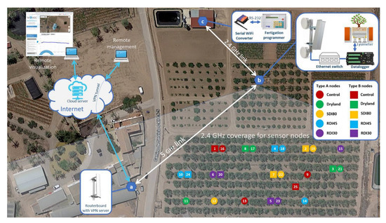
Figure 1.
WSN infrastructure of the experimental orchard.
Thanks to this infrastructure, the sensor nodes of the almond plot send the data to a server hosted in the cloud, which provides all the necessary services for its visualization from any personal computer or mobile device. This application allows real-time visualization, logging and querying of historical data, and alarm reporting among other features.
2.4. Agronomic Sensors
To allow for real-time monitoring, several sensors were connected to wireless nodes (see Table 1):

Table 1.
Overview of the sensors used in the plot.
- A total of four sensors per replicate (twelve in total) deployed as follows: two volumetric soil water content sensors (10HS, Decagon devices, Inc., Pullman, WA, USA) and two matric potential of soil water sensors (MPS-6, Decagon devices, Inc., Pullman, WA, USA), installed at 23 cm from each dripper and 25 and 45 cm depth located under the canopy and along the tree drip lines.
- A total of two linear variable displacement transducer sensors (LVDT, Model DF ± 2.5 mm, Solartron Metrology, Bognor Regis, UK) per replicate (six in total) were installed on the main tree branch for measuring micrometric branch diameter variations.
- A total of two infrared radiometer sensors (IR120, Campbell Scientific Inc., USA) per treatment were mounted on wooden poles and installed at 0.5–1.0 m over the trees canopy for monitoring canopy temperature.
- A total of four climatic sensors (VP4, Decagon devices, Inc., Pullman, WA USA) were installed to record air temperature, relative humidity and vapor pressure deficit.
2.5. Sensor Nodes
From the hardware/software point of view, there are two types of nodes: type A and type B, with different subtypes according to the sensors connected to them. The electronics of nodes A and B are housed inside a 120 × 120 × 90 mm IP65 box (G279C, Gainta AEK GmbH—Electrical Enclosures, Frankfurt, Germany). The power supply system consists of a 3.7 V, 3000 mAh Li-ion rechargeable battery, charged by an 80 × 80 mm solar panel (5 V, 0.8 W). Figure 2 shows pictures of both types of node installed in the field.
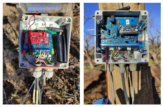
Figure 2.
Pictures of type-A (left) and type-B (right) nodes.
Table 2 shows the 25 nodes installed in the plot (see Figure 1), detailing, for each of them, the type it belongs to, the replicate, the irrigation treatment it is monitoring and the sensors connected to it.
Table 2.
Description of the deployed nodes.
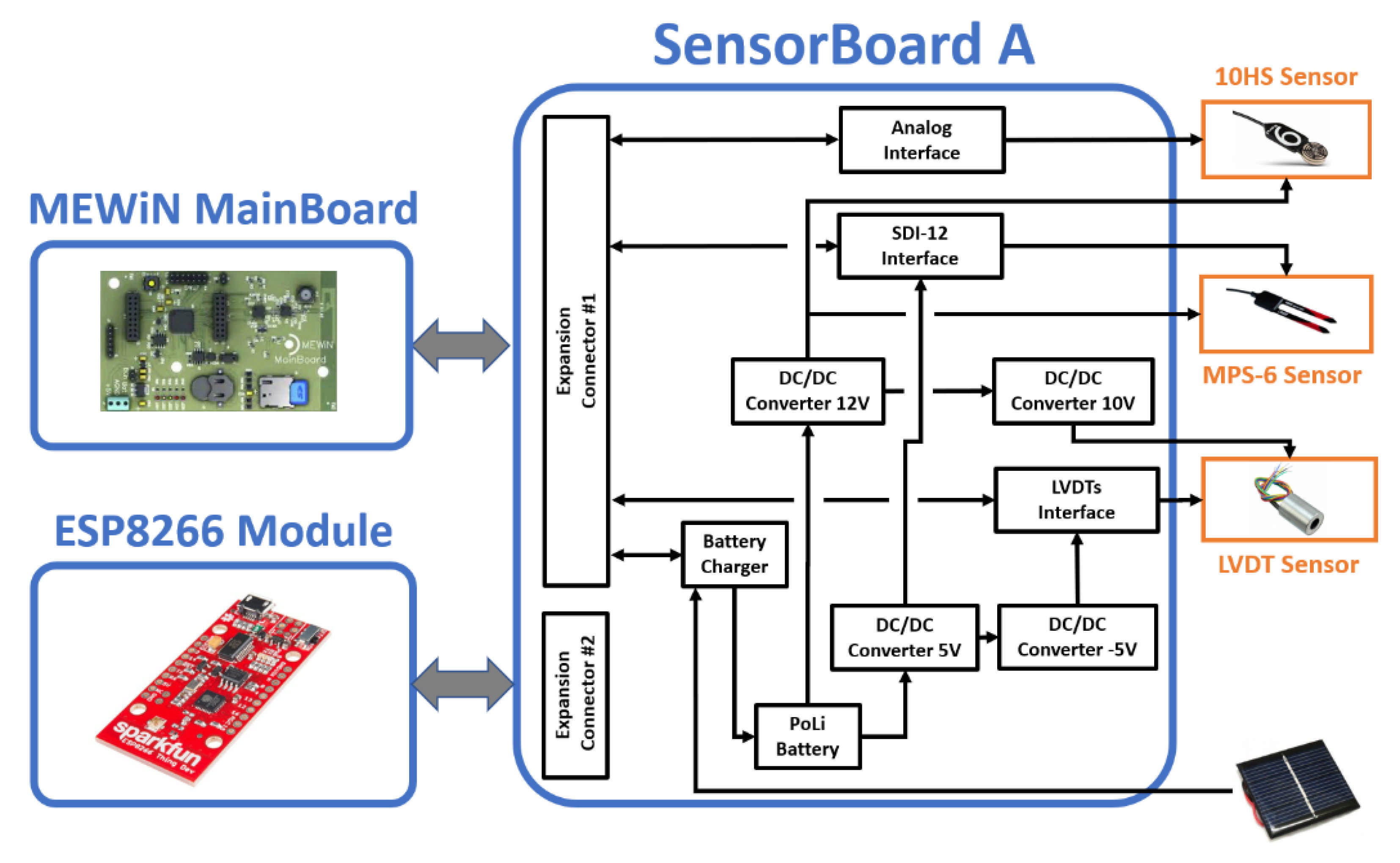
The hardware of the type A node (see Figure 3) is based on a wireless datalogger designed by our research group for PA applications (MEWiN MainBoard) [20]. For the signal conditioning from the sensors, an interface board (SensorBoard A) has been designed, connected to the first one by means of expansion connectors. An ESP8266 microcontroller (Esspressif Systems Co. LTD., Shanghai, China) with WiFi communication capability is also plugged to the SensorBoard A.
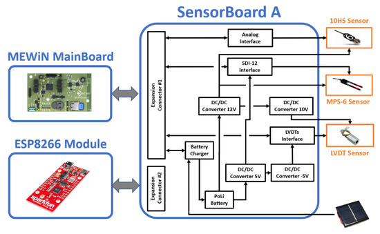
Figure 3.
Block diagram of type-A node.
The SensorBoard A consists of four DC/DC voltage converters (12, 10, 5 and −5 V), required to supply the sensors and to guarantee the operation of the different interfaces on the board: one for SDI12 sensors, another for radial dendrometers and one for analogue sensors (0–3 V). Finally, the board includes a circuit for the management of the rechargeable battery that supplies the power to the node.
The type B Node is similar to type A, but it is based on the use of a Wipy 3.0 (Pycom©, London, UK) (see Figure 4).
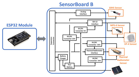
Figure 4.
Block diagram of type-B node.
The SensorBoard B includes four DC/DC voltage converters (12, 10, −3.3 and −2.5 V), required to supply the sensors and to guarantee the operation of the different interfaces on the board: one for SDI12 sensors, another for thermal radiometers and one for analogue sensors (0–3 V). Finally, the board includes a circuit for the management of the rechargeable battery that supplies the power to the node.
The software of the nodes was developed using the MicroPython programming language and a variety of open source libraries for Wi-Fi connectivity and sensor reading, among others. For some tasks, such as data acquisition from SDI-12 sensors, specific algorithms were developed.
2.6. Time Synchronization
One of the requirements established by the agronomists for this study was that all the nodes should take the sensor measurements at the same time every 15 min so that they could be compared. Therefore, a synchronization algorithm was implemented: Once a day, the nodes connected to a time server (NTP) and update their real-time clock (RTC), which is very inaccurate (it has a daily drift of approximately 50 s). This inaccuracy, together with the drift of the internal timer in deep sleep mode (about 0.3%), generated a time drift that resulted in desynchronized measurements between nodes. To solve this problem, a time correction algorithm was developed. This algorithm determined the time the system requires to perform the measuring and data sending processes, working out the remaining time needed to be in deep sleep mode before waking up at the exact minute defined by the sampling period. In this deployment, measurements were performed every 15 min (minute 0, 15, 30 and 45 of each hour) and measurements were sent every 30 min (minute 0 and 30 of each hour).
3. Results and Discussion
After the functional validation, in view of the importance of achieving the maximum autonomy, the current consumption of each of the node types was measured in the field. The measurements were performed with a data acquisition card (USB-6008, National Instruments Corp., Austin, TX, USA) that measured the voltage drop at a 1 Ohm shunt resistor placed in series with the battery that powered the node. The analog input of the card was configured in differential mode in the range of ±1 V and the acquisition was carried out in continuous mode at 1 kHz obtaining the averages every 0.25 s. In this mode, the card has a 12-bit resolution (equivalent to 0.48 mA) and an absolute precision at 25 °C of 1.53 mV (1.53 mA in current).
For both type A and type B nodes, consumption tests were performed for the three possible operating modes, (i) the node connects to synchronize the date and time, collects data from the sensors and sends them to the server (this is the most energy-demanding operating mode and is therefore programmed to occur only every 24 h), (ii) the node collects data and sends them to the server (occurs every 30 min) and (iii) the node collects data and stores them in the memory card waiting for the next connection to the server (occurs in the middle of the period between sending events, i.e., 15 min later).
3.1. Consumption of Type A Nodes
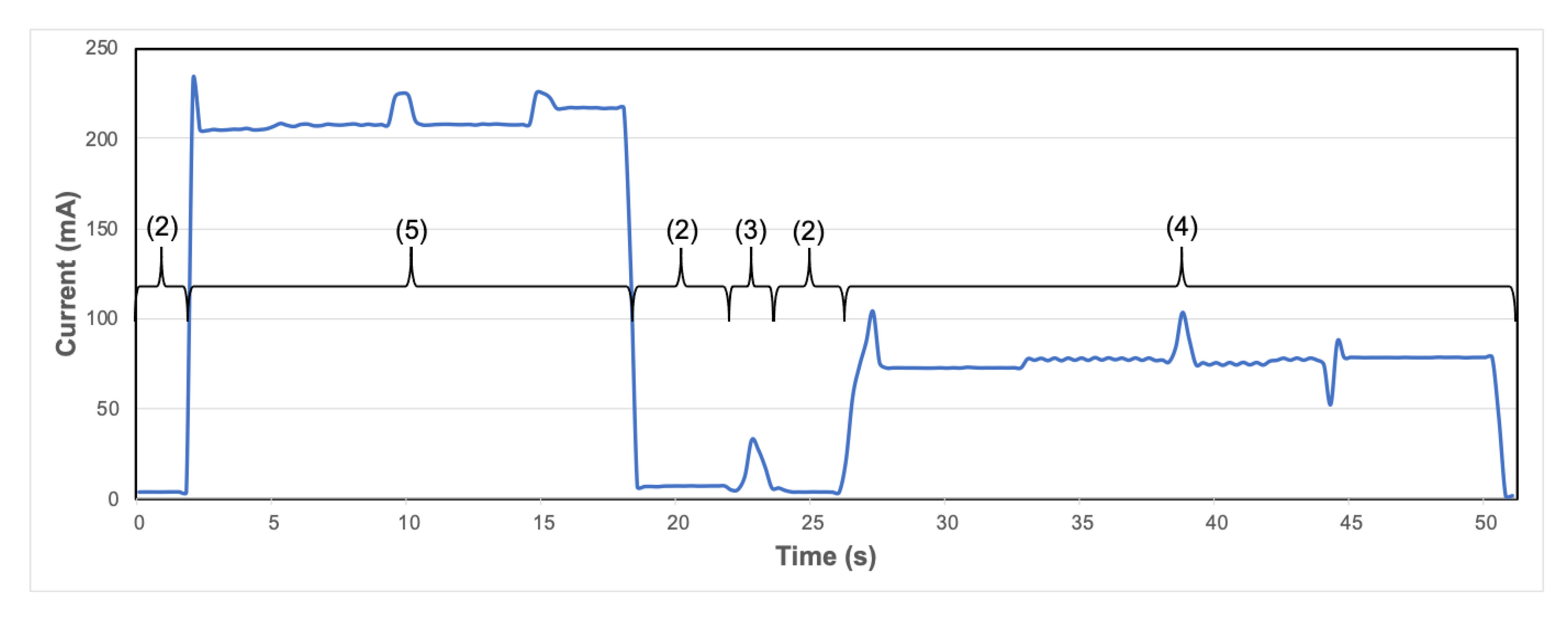
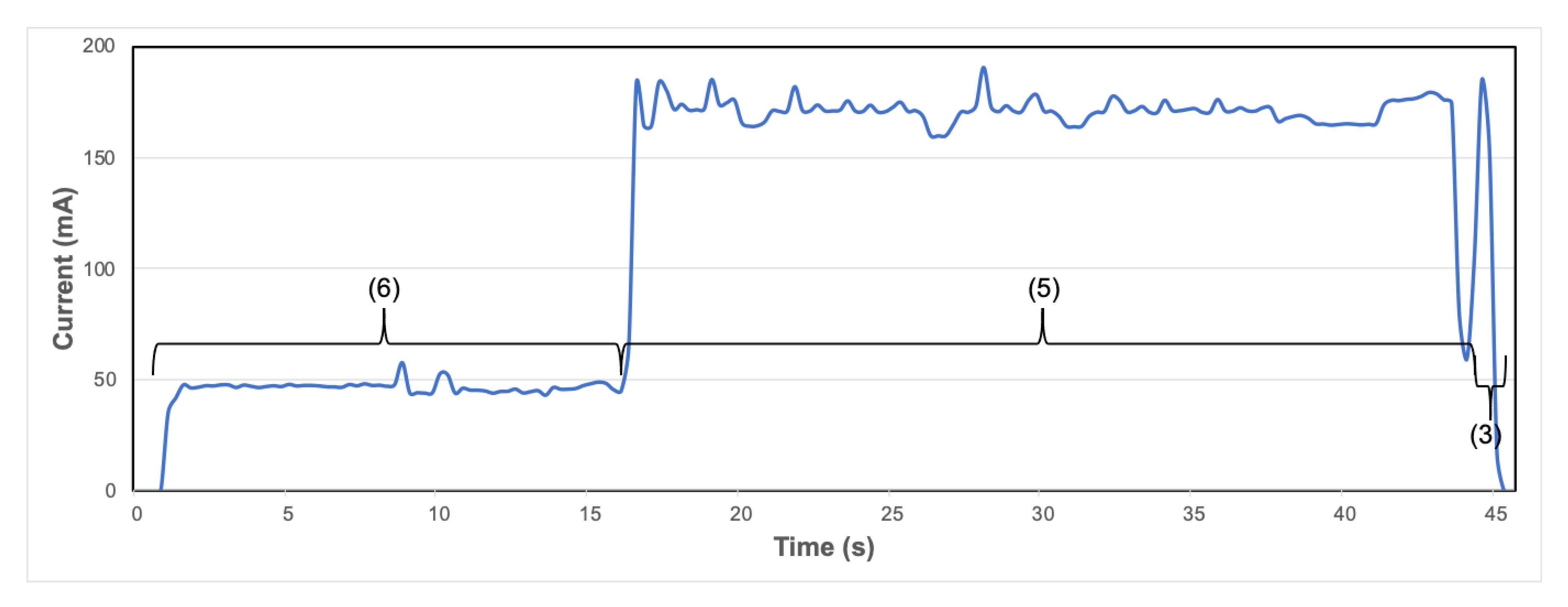
Node type A had a standby consumption of 1.1 mA. Figure 5 shows the current required in each of the states through which the node passes in operating mode (i). The measured current and the duration of each of these states are shown in Table 3. With these values, taking into account the standby current, the total consumption of the mode has been calculated with Equation (1).
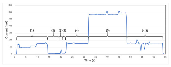
Figure 5.
Node A—mode (i): NTP sync, sensor reading and data sending (once every 24 h).
Table 3.
Description of functional states of node A—mode (i).
The function of each state is indicated in its description (Table 3). In state 2 (task signaling), the node displays information about the task it is executing by means of a lighting sequence of four LEDs. This information helps the user to perform maintenance and commissioning tasks in the field.
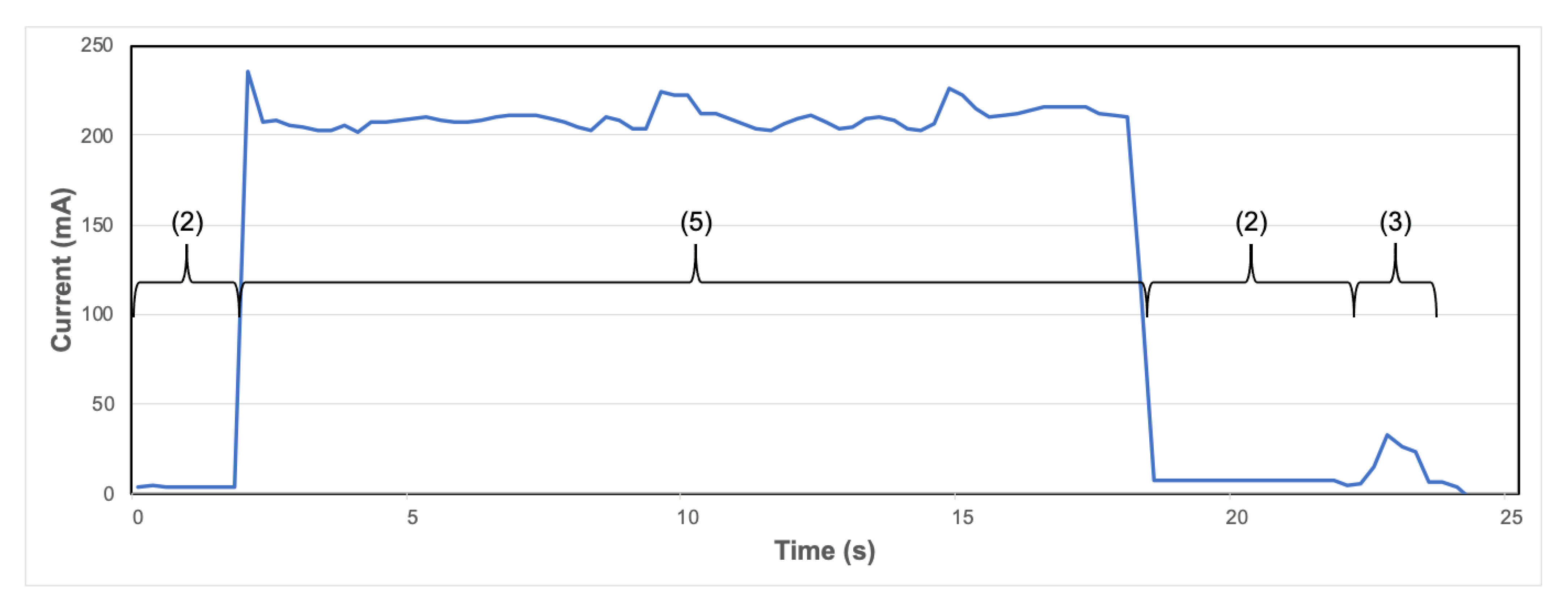
Figure 6 and Figure 7, Table 4 and Table 5, and Equations (2) and (3) show similar calculations for the other two modes of operation of the node: modes (ii) and (iii). Note that mode (i) occurs once a day, i.e., every 86,400 s (24·60·60) and modes ii and iii every 30 min, i.e., every 1800 s (30 × 60).
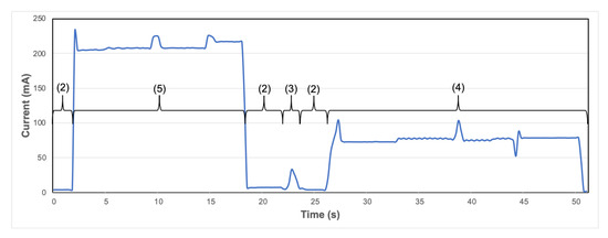
Figure 6.
Node A—mode (ii): Sensor reading with data sending (every 30 min).
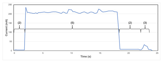
Figure 7.
Node A—mode (iii): Sensor reading without data sending (every 30 min).
Table 4.
Description of functional states of node A—mode (ii).
Table 5.
Description of functional states of node A—mode (iii).
Once the total consumption current of each of the operating modes has been determined, taking into account the standby current and the capacity of the battery installed in the nodes, it is possible to calculate (Equation (4)) the autonomy (in days) provided that the battery is not charged by any means.
3.2. Consumption of Type B Nodes
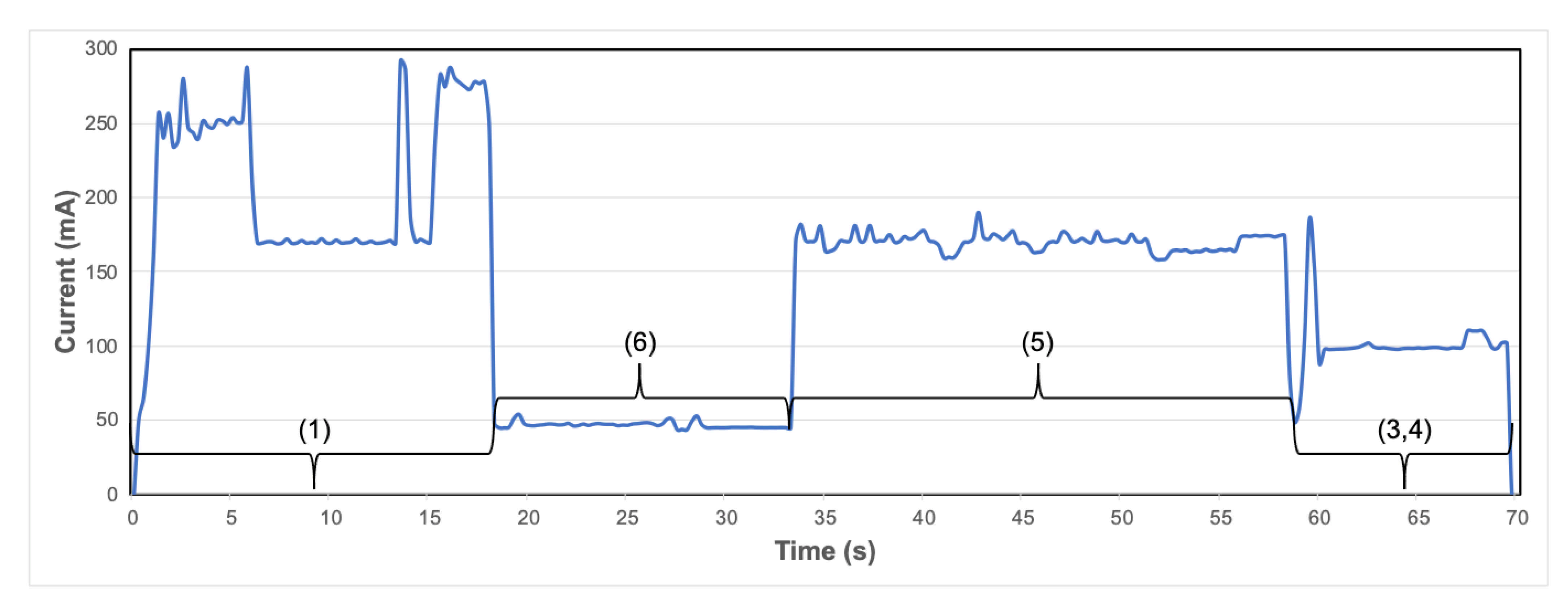
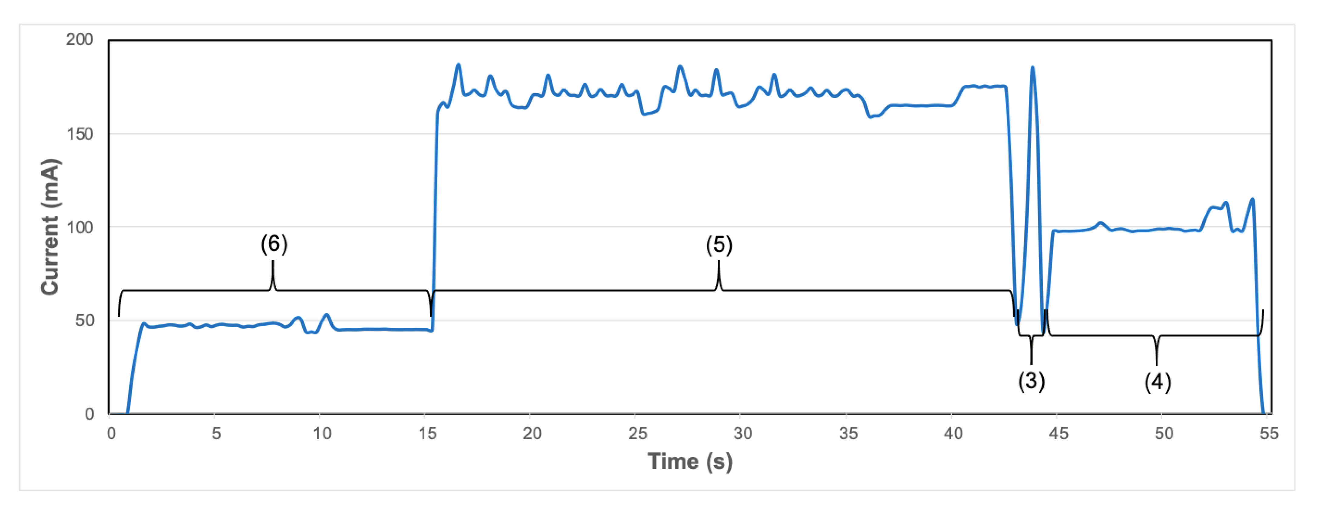
The same measurements and calculations made for node A were carried out for type B node. These calculations are shown in Figure 8, Figure 9 and Figure 10, Table 6, Table 7 and Table 8, and Equations (5)–(7). In this case, node B had a standby current of 1.5 mA.
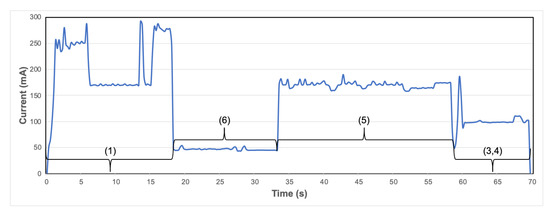
Figure 8.
Node B—mode (i): NTP sync, sensor reading and data sending (once every 24 h).
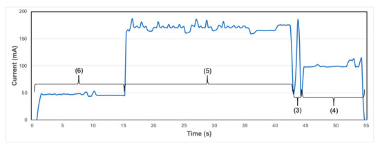
Figure 9.
Node B—mode (ii): Sensor reading and data sending (every 30 min).
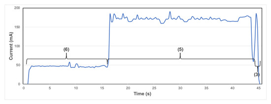
Figure 10.
Node B—mode (iii): Sensor reading without data sending mode (every 30 min).
Table 6.
Description of functional states of node B—mode (i).
Table 7.
Description of functional states of node B—mode (ii).
Table 8.
Description of functional states of node B—mode (iii).
The autonomy of node B, provided that the battery is not charged by any means, is depicted in Equation (8).
3.3. Sensor Data Validation
In order to demonstrate the usefulness and viability of the deployed network of nodes, data registered over a significant period of time from an agronomic and sensor network reliability point of view are shown below.
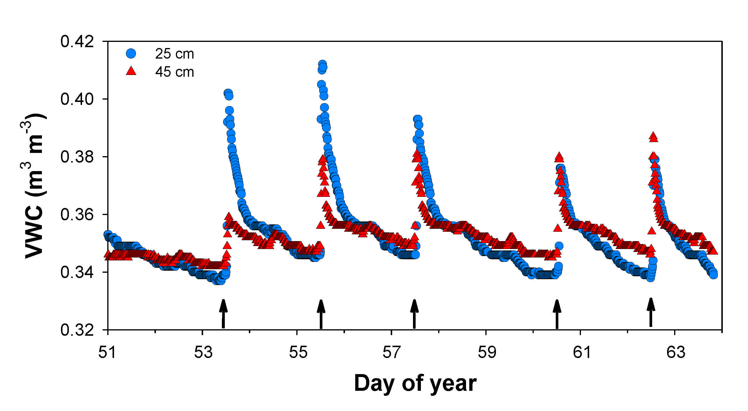
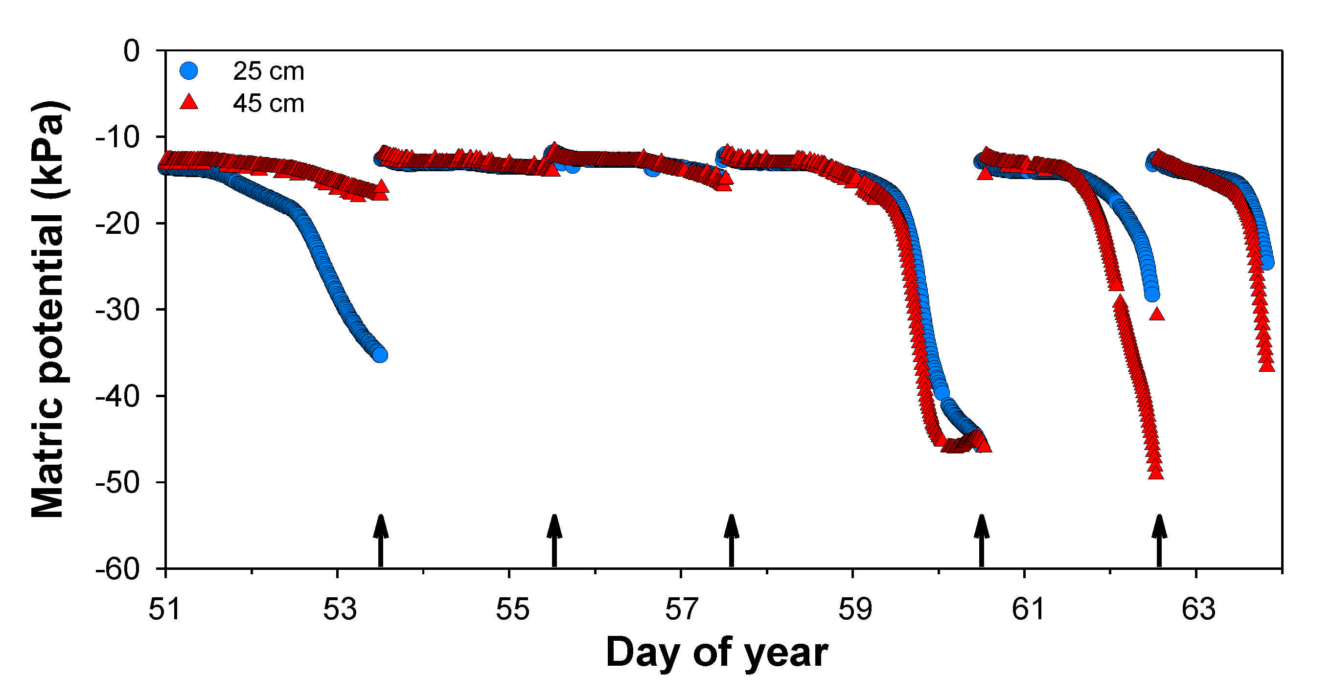
Figure 11 shows the evolution of the VWC at both 25 and 45 cm depth, measured by 10HS sensors (node 04). Irrigation was scheduled every two or three days at 11 a.m. and it took 2 h. VWC values ranged between 0.413 and 0.336 m3 m−3 during the test period. The maximum values were reached during the irrigation events. After the irrigation events, VWC values fell due to infiltration and they stabilized at values close to 0.358 m3 m−3. The information registered by MPS-6 sensors (Figure 12) was complementary to that obtained by 10HS sensors (Figure 11). In each irrigation event and depth, the value increased until it was close to −7 kPa, being considered this as field capacity [48]. The falls of MPS-6 sensors were steeper than those registered by 10HS sensors. Both types of sensors detected the irrigation events between 1 and 2 h after irrigation events started in both depths. During the test period, evaporative demand increased strongly, going from a reference crop evapotranspiration of 2.5 to 4.0 mm d−1 at the end of the study period, which accelerated the falls of the VWC and soil matric potential values, as well as it showed a greater drop in values. The values showed both types of sensors at saturation level were similar to those reported by [49] on similar texture soil.

Figure 11.
Evolution of VWC sensors at 25 and 45 cm depth measured by node 04 with 10HS sensors (year 2020). The arrows indicate the irrigation events.
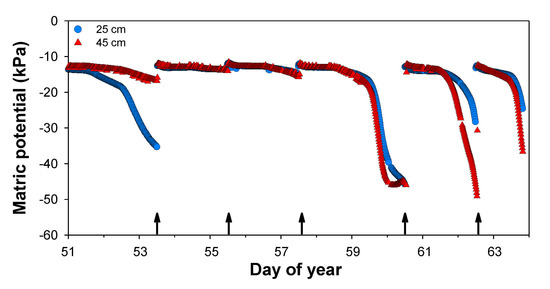
Figure 12.
Evolution of matric potential at 25 and 45 cm depth measured by node 04 with MPS-6 sensors (year 2020). The arrows indicate the irrigation events.
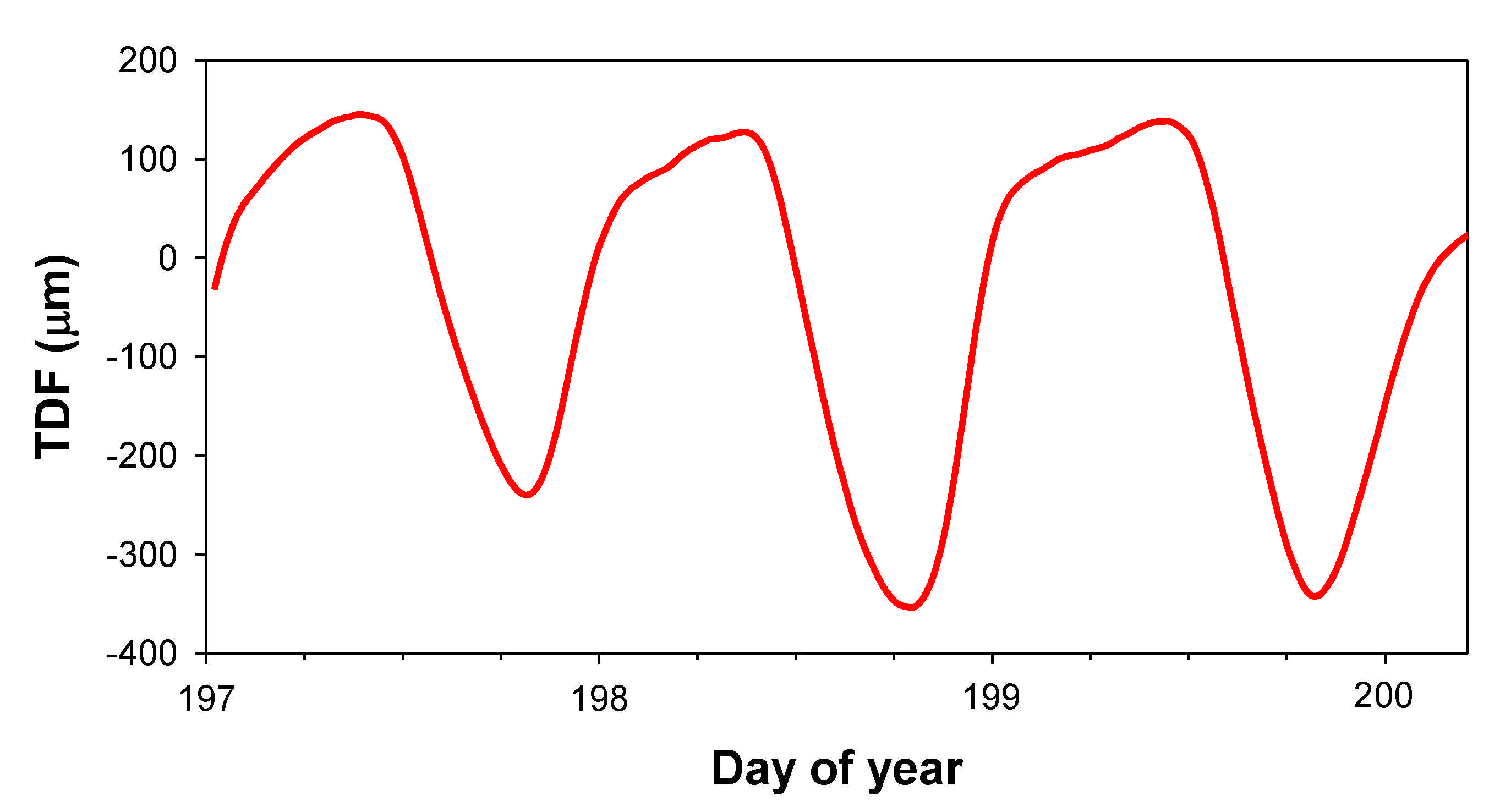
Additionally, the nodes automatically and continuously monitored plant water status with LVDT sensors. Figure 13 shows trunk diameter fluctuations (TDF) where the daily cycle of shrinkage for RDI30 for three consecutive days can be observed. The maximum trunk diameter (MXTD) was reached at the beginning of the day and the minimum trunk diameter (MNTD) was recorded during the afternoon. From data obtained from TDF, two indices were calculated to establish plant water status. The daily trunk shrinkage values, calculated as the difference between MXDT and MNTD on the same day, were 271, 411 and 292 μm for three consecutive days, respectively. The trunk growth rate values were calculated as the difference between MXTD of two consecutive days. In general, they were close to 0 μm throughout the period considered. The trend and values obtained were in agreement with those reported by [50,51].
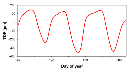
Figure 13.
Evolution of trunk diameter fluctuations (TDF) of the RDI30 treatment trees during deficit irrigation period (stage IV). The data was stored by node 23 equipped with linear variable displacement transducer sensors (year 2019).
3.4. Reliability of the Nodes
In general terms, the performance of the nodes was satisfactory. Obviously, the installation required periodic maintenance tasks, such as cleaning the solar panels, and eventual interventions due to occasional failures in the hardware of the nodes.
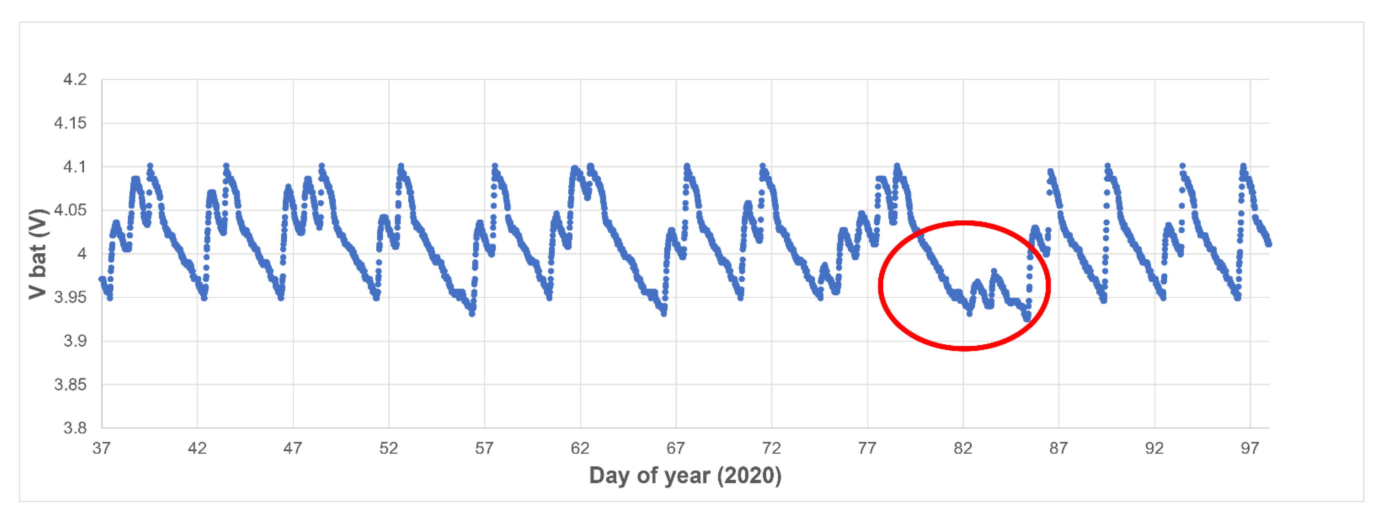
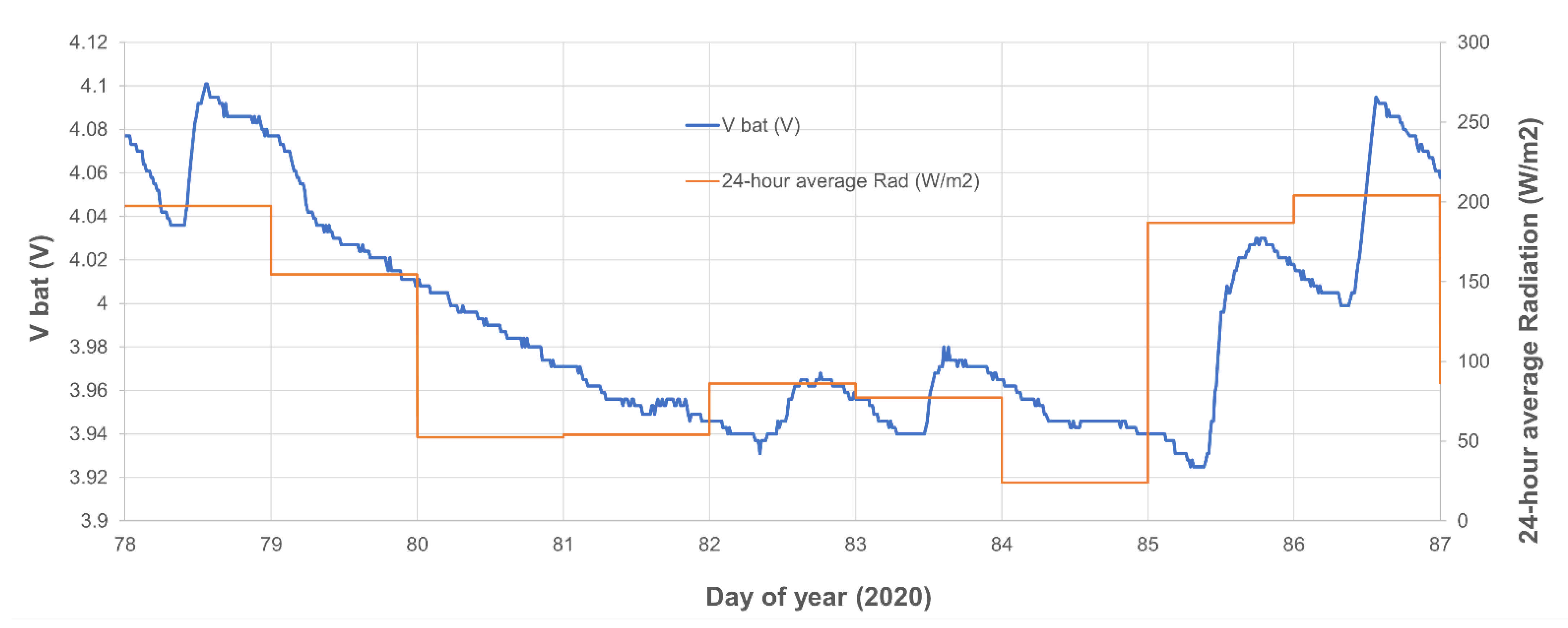
The evolution of the battery voltage of the nodes is a useful indicator of the “health” of the node. As an example, Figure 14 shows the evolution of the battery voltage of one of the nodes (node 25) in typical conditions. As can be seen, the battery management algorithm starts the charge when the voltage falls below the lower threshold (3.95 V) and stops when the upper threshold is reached (4.1 V). In this way, it works within the optimum voltage range for the battery and reduces the charge cycles, extending its useful life. During the charge there are different voltage peaks corresponding to the daylight hours (the solar panel supplies charge) and the hours of darkness during the night (there is no photovoltaic generation and the battery discharges due to the node consumption). The “discrepancy” that appears between days 82 and 87 (22 and 27 March 2020) corresponds to days when solar radiation was lower due to the existence of cloudiness (see Figure 15).

Figure 14.
Typical behavior of the battery voltage in a node without operational problems.
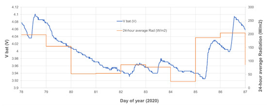
Figure 15.
Battery voltage (node 25) vs. daily average radiation (source: http://siam.imida.es/ Agro-Meteorological Weather Station CA12-La Palma, accessed on 6 April 2020). Cloudy days.
3.5. Typical Node Failures
Among the common problems detected during the operation of the deployment, the most frequent were those that led to the exhaustion or destruction of the battery. The usual reasons were (i) overheating due to the high temperatures reached inside the box in summer, (ii) dirt or ageing of the solar panels and (iii) natural ageing of the batteries as they reached the end of their lifespan.
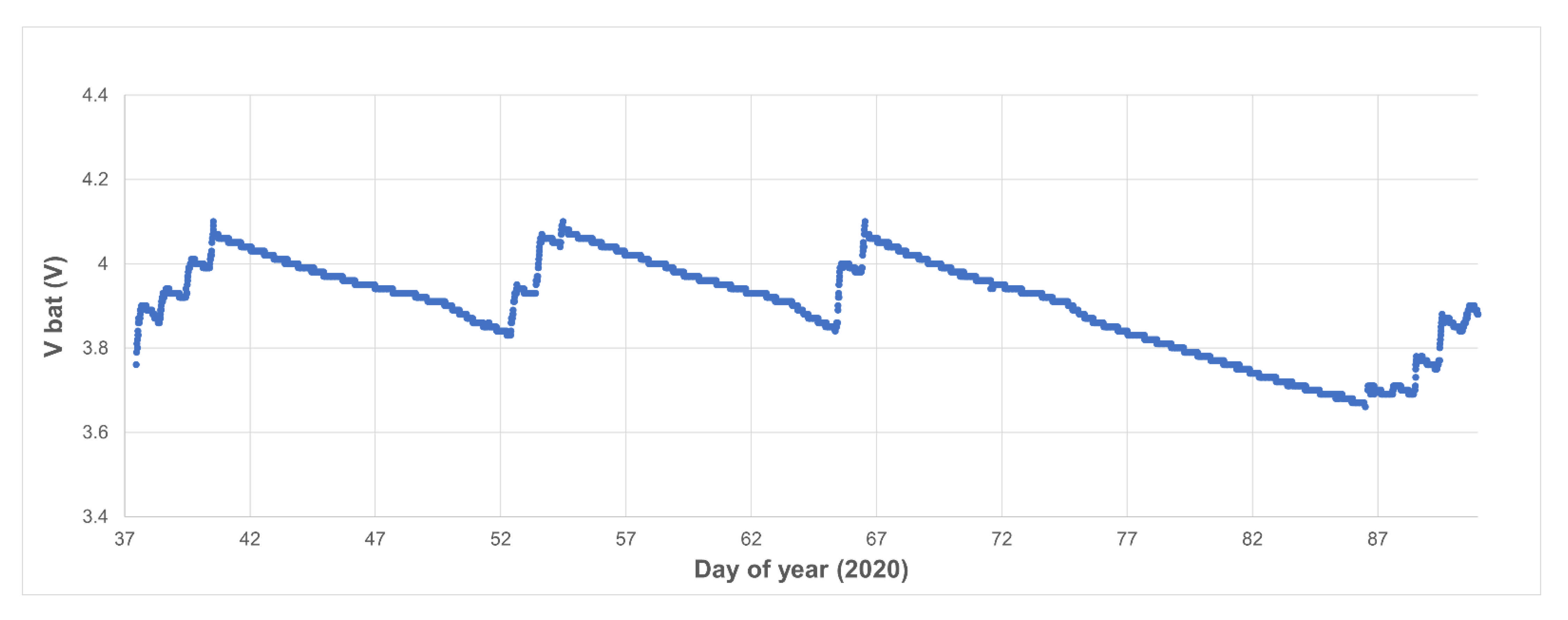
Figure 16 presents the evolution of the battery voltage of node 23. As can be seen, between 7 and 27 March there was a prolonged discharge due to the ageing of the panel, which stopped charging (this was later verified in a field intervention). Once the solar panel was replaced on the 27th, the node started charging again. It is worth noting that from this graph it is possible to extract very interesting information: due to the failure of the panel, the node showed an autonomy of approximately 20 days, which validates the theoretical calculations indicated in the section of consumption and autonomy estimation of the nodes.

Figure 16.
Evolution of the battery voltage of node 23.
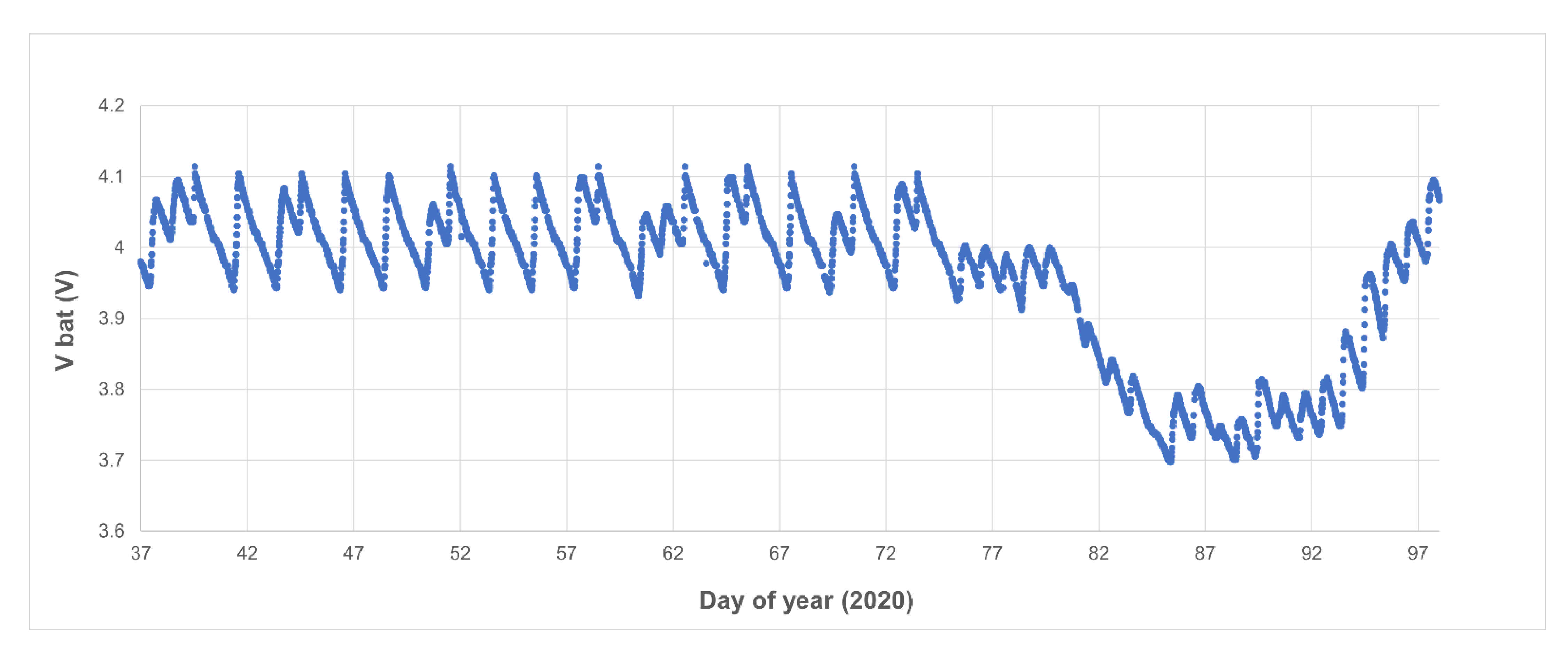
Figure 17 and Figure 18 depict failures in two other nodes due to dirt on the solar panels (mainly dust and bird droppings). In the case of node 5 (Figure 17), it can be seen that since 15 March, there were successive loads that did not reach the upper threshold. From 21 March, the panel did not supply the required current to increase the battery charge, whose voltage started a downward trend until 25 March, the day on which the panel was cleaned, and the node recovered. In the case of node 4 (Figure 18), the node never managed to reach the upper threshold because the panel current was not sufficient, so on 24 March, the voltage fell below the minimum operating voltage and the node stopped transmitting.
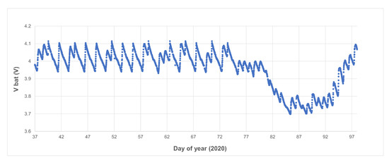
Figure 17.
Evolution of the battery voltage of a node with a dirty panel (node 05).
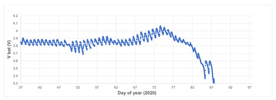
Figure 18.
Evolution of the battery voltage of a node with a dirty panel (node 04).
4. Conclusions
The results described in this work demonstrate the viability of using new or existing Wi-Fi infrastructures for the collection of agronomic data with low-cost nodes in deployments for taking measurements over long periods of time. Although some authors argue that Wi-Fi is not the most suitable technology for WSN in PA, the application of techniques to reduce consumption and the use of energy harvesting methods (solar panels) allows for virtually unlimited node operating autonomy. Consequently, this work demonstrates that, properly managing the energy demand, WSN deployment using Wi-Fi is feasible and even advantageous in installations where Wi-Fi coverage is already available or a major investment in the communications infrastructure is not desired. In addition, the use of Wi-Fi is particularly convenient when using multi-node deployments on the same plot (high density), e.g., in research trials where it is necessary to replicate measurements in several locations to minimize variability, and also to perform them with different parameters to evaluate the performance of irrigation strategies on a given crop.
In addition, time synchronization techniques have been implemented to ensure time alignment of the data measured by the sensors. This facilitates its subsequent analysis for the realization of agronomic studies that relate the different irrigation treatments with the state of the plant and the crop yield.
Likewise, the experimental installation described in this work has demonstrated the reliability of the nodes, sensors and communications infrastructure used. The experimental results have shown that, although wireless networks require less installation and maintenance tasks than wired ones, they do need programmed servicing interventions and occasional troubleshooting.
Next steps would involve the integration of nodes with other communication technologies such as LoRa to carry out studies to compare the advantages and disadvantages of each technology.
Author Contributions
Conceptualization, R.T.-S. and M.J.-B.; methodology, R.D.-M. and P.J.B.-R.; software, A.T.-M., F.S.-V. and M.J.-B.; validation, P.J.B.-R., F.S.-V. and A.T.-M.; formal analysis, F.S.-V. and P.J.B.-R.; investigation, R.D.-M. and P.J.B.-R.; resources, R.T.-S. and R.D.-M.; data curation, M.J.-B. and A.T.-M.; writing—original draft preparation, M.J.-B.; writing—review and editing, M.J.-B., P.J.B.-R., F.S.-V. and R.T.-S.; visualization, M.J.-B.; supervision, R.T.-S. and R.D.-M.; project administration, R.T.-S. and R.D.-M.; funding acquisition, R.T.-S. and R.D.-M. All authors have read and agreed to the published version of the manuscript.
Funding
This research was funded by the Spanish Science and Innovation Ministry (MICIIN) and the European Agricultural Funds for Rural Development, grant numbers: AGL2016-77282-C3-3-R and PID2019-106226RB-C22/AEI/10.13039/501100011033.
Conflicts of Interest
The authors declare no conflict of interest.
References
- Food and Agriculture Organization of the United Nations. Deficit Irrigation Practices; Food and Agriculture Organization of the United Nations: Rome, Italy, 2002; Volume 22. [Google Scholar]
- Yu, L.; Zhao, X.; Gao, X.; Siddique, K.H.M. Improving/maintaining water-use efficiency and yield of wheat by deficit irrigation: A global meta-analysis. Agric. Water Manag. 2020, 228, 105906. [Google Scholar] [CrossRef]
- Pardo, J.J.; Martínez-Romero, A.; Léllis, B.C.; Tarjuelo, J.M.; Domínguez, A. Effect of the optimized regulated deficit irrigation methodology on water use in barley under semiarid conditions. Agric. Water Manag. 2020, 228, 105925. [Google Scholar] [CrossRef]
- Kang, S.; Zhang, L.; Liang, Y.; Hu, X.; Cai, H.; Gu, B. Effects of limited irrigation on yield and water use efficiency of winter wheat in the Loess Plateau of China. Agric. Water Manag. 2002, 55, 203–216. [Google Scholar] [CrossRef]
- Du, T.; Kang, S.; Zhang, J.; Davies, W.J. Deficit irrigation and sustainable water-resource strategies in agriculture for China’s food security. J. Exp. Bot. 2015, 66, 2253–2269. [Google Scholar] [CrossRef]
- Blanco, V.; Torres-Sánchez, R.; Blaya-Ros, P.J.; Pérez-Pastor, A.; Domingo, R. Vegetative and reproductive response of ‘Prime Giant’ sweet cherry trees to regulated deficit irrigation. Sci. Hortic. 2019, 249, 478–489. [Google Scholar] [CrossRef]
- Haule, J.; Michael, K. Deployment of wireless sensor networks (WSN) in automated irrigation management and scheduling systems: A review. In Proceedings of the 2nd Pan African International Conference on Science, Computing and Telecommunications, PACT 2014, Arusha, Tanzania, 14–18 July 2014; pp. 86–91. [Google Scholar]
- Wang, N.; Li, Z. Wireless sensor networks (WSNs) in the agricultural and food industries. In Robotics and Automation in the Food Industry: Current and Future Technologies; Elsevier Ltd.: Amsterdam, The Netherlands, 2012; pp. 171–199. ISBN 9781845698010. [Google Scholar]
- Balendonck, J.; Hemming, J.; van Tuijl, B.A.J.; Incrocci, L.; Pardossi, A.; Marzialetti, P. Sensors and wireless sensor networks for irrigation management under deficit conditions (FLOW-AID). In Proceedings of the International Conference on Agricultural Engineering (AgEng 2008), Hersonissos, Crete, 23–25 June 2008; pp. 3–452. [Google Scholar]
- Elijah, O.; Rahman, T.A.; Orikumhi, I.; Leow, C.Y.; Hindia, M.N. An Overview of Internet of Things (IoT) and Data Analytics in Agriculture: Benefits and Challenges. IEEE Internet Things J. 2018, 5, 3758–3773. [Google Scholar] [CrossRef]
- Jawad, H.M.; Nordin, R.; Gharghan, S.K.; Jawad, A.M.; Ismail, M. Energy-efficient wireless sensor networks for precision agriculture: A review. Sensors 2017, 17, 1781. [Google Scholar] [CrossRef] [Green Version]
- Aqeel-ur-Rehman; Abbasi, A.Z.; Islam, N.; Shaikh, Z.A. A review of wireless sensors and networks’ applications in agriculture. Comput. Stand. Interfaces 2014, 36, 263–270. [Google Scholar] [CrossRef]
- De Oliveira, K.V.; Castelli, H.M.E.; Montebeller, S.J.; Avancini, T.G.P. Wireless Sensor Network for Smart Agriculture Using ZigBee Protocol. In Proceedings of the 2017 IEEE 1st Summer School on Smart Cities, S3C 2017—Proceedings, Natal, Brazil, 6–11 August 2017; pp. 61–66. [Google Scholar]
- Prakash, S. Zigbee based wireless sensor network architecture for agriculture applications. In Proceedings of the 3rd International Conference on Smart Systems and Inventive Technology, ICSSIT 2020, Tirunelveli, India, 20–22 August 2020; pp. 709–712. [Google Scholar]
- Rodríguez, S.; Gualotuña, T.; Grilo, C. A System for the Monitoring and Predicting of Data in Precision Agriculture in a Rose Greenhouse Based on Wireless Sensor Networks. In Proceedings of the Procedia Computer Science; Elsevier B.V.: Amsterdam, The Netherlands, 2017; Volume 121, pp. 306–313. [Google Scholar]
- Sahitya, G.; Balaji, N.; Naidu, C.D. Wireless sensor network for smart agriculture. In Proceedings of the 2016 2nd International Conference on Applied and Theoretical Computing and Communication Technology, iCATccT 2016, Bengaluru, Karnataka, India, 21–23 July 2016; pp. 488–493. [Google Scholar]
- Samijayani, O.N.; Darwis, R.; Rahmatia, S.; Mujadin, A.; Astharini, D. Hybrid ZigBee and WiFi Wireless Sensor Networks for Hydroponic Monitoring. In Proceedings of the 2nd International Conference on Electrical, Communication and Computer Engineering, ICECCE 2020, Istanbul, Turkey, 12–13 June 2020. [Google Scholar]
- Xiao, J.; Li, J.T. Design and implementation of intelligent temperature and humidity monitoring system based on ZigBee and WiFi. In Proceedings of the Procedia Computer Science; Elsevier B.V.: Amsterdam, The Netherlands, 2020; Volume 166, pp. 419–422. [Google Scholar]
- Wang, Z.; Jiang, Z.; Hu, J.; Song, T.; Cao, Z. Research on Agricultural Environment Information Collection System Based on LoRa. In Proceedings of the 2018 IEEE 4th International Conference on Computer and Communications (ICCC), Chengdu, China, 7–10 December 2018; pp. 2441–2445. [Google Scholar]
- Albaladejo, C.; Soto, F.; Torres, R.; Sánchez, P.; López, J.A. A Low-Cost Sensor Buoy System for Monitoring Shallow Marine Environments. Sensors 2012, 12, 9613–9634. [Google Scholar] [CrossRef]
- López, J.; Soto, F.; Sánchez, P.; Iborra, A.; Suardiaz, J.; Vera, J. Development of a Sensor Node for Precision Horticulture. Sensors 2009, 9, 3240–3255. [Google Scholar] [CrossRef]
- Navarro-Hellín, H.; Torres-Sánchez, R.; Soto-Valles, F.; Albaladejo-Pérez, C.; López-Riquelme, J.A.; Domingo-Miguel, R. A wireless sensors architecture for efficient irrigation water management. Agric. Water Manag. 2015, 151, 64–74. [Google Scholar] [CrossRef] [Green Version]
- Riquelme, J.A.L.; Soto, F.; Suardíaz, J.; Sánchez, P.; Iborra, A.; Vera, J.A. Wireless Sensor Networks for precision horticulture in Southern Spain. Comput. Electron. Agric. 2009, 68, 25–35. [Google Scholar] [CrossRef]
- Alahi, M.E.E.; Pereira-Ishak, N.; Mukhopadhyay, S.C.; Burkitt, L. An Internet-of-Things Enabled Smart Sensing System for Nitrate Monitoring. IEEE Internet Things J. 2018, 5, 4409–4417. [Google Scholar] [CrossRef]
- Bhattacherjee, S.S.; Shreeshan, S.; Priyanka, G.; Jadhav, A.R.; Rajalakshmi, P.; Kholova, J. Cloud based Low-Power Long-Range IoT Network for Soil Moisture monitoring in Agriculture. In Proceedings of the 2020 IEEE Sensors Applications Symposium (SAS), Kuala Lumpur, Malaysia, 9–11 March 2020; pp. 1–5. [Google Scholar]
- Jing, L.; Wei, Y. Intelligent Agriculture System Based on LoRa and Qt Technology. In Proceedings of the 31st Chinese Control and Decision Conference, CCDC 2019, Nanchang, China, 3–5 June 2019; pp. 4755–4760. [Google Scholar]
- Kokten, E.; Caliskan, B.C.; Karamzadeh, S.; Soyak, E.G. Low-Powered Agriculture IoT Systems with LoRa. In Proceedings of the 2020 IEEE Microwave Theory and Techniques in Wireless Communications (MTTW), Riga, Latvia, 1–2 October 2020; pp. 178–183. [Google Scholar]
- Ma, Y.W.; Chen, J.L. Toward intelligent agriculture service platform with lora-based wireless sensor network. In Proceedings of the 4th IEEE International Conference on Applied System Innovation 2018, ICASI 2018, Chiba, Japan, 13–17 April 2018; pp. 204–207. [Google Scholar]
- Mohammed, T.S.; Khan, O.F.; Al-Bazi, A. A Novel Algorithm Based on LoRa Technology for Open-Field and Protected Agriculture Smart Irrigation System. In Proceedings of the 2019 2nd IEEE Middle East and North Africa COMMunications Conference, MENACOMM 2019, Manama, Bahrain, 19–21 November 2019. [Google Scholar]
- Nursyahid, A.; Aprilian, T.; Setyawan, T.A.; Helmy; Nugroho, A.S.; Susilo, D. Automatic sprinkler system for water efficiency based on lora network. In Proceedings of the 2019 6th International Conference on Information Technology, Computer and Electrical Engineering, ICITACEE 2019, Semarang, Indonesia, 26–27 September 2019.
- Sarker, V.K.; Queralta, J.P.; Gia, T.N.; Tenhunen, H.; Westerlund, T. A survey on LoRa for IoT: Integrating edge computing. In Proceedings of the 2019 4th International Conference on Fog and Mobile Edge Computing, FMEC 2019, Rome, Italy, 10–13 June 2019; pp. 295–300. [Google Scholar]
- Usmonov, M.; Gregoretti, F. Design and implementation of a LoRa based wireless control for drip irrigation systems. In Proceedings of the 2017 2nd International Conference on Robotics and Automation Engineering, ICRAE 2017, Shanghai, China, 29–31 December 2017; Volume 2017, pp. 248–253. [Google Scholar]
- Ahmed, N.; De, D.; Hussain, I. Internet of Things (IoT) for Smart Precision Agriculture and Farming in Rural Areas. IEEE Internet Things J. 2018, 5, 4890–4899. [Google Scholar] [CrossRef]
- Liang, M.H.; He, Y.F.; Chen, L.J.; Du, S.F. Greenhouse Environment dynamic Monitoring system based on WIFI. IFAC-PapersOnLine 2018, 51, 736–740. [Google Scholar] [CrossRef]
- Ndzi, D.L.; Harun, A.; Ramli, F.M.; Kamarudin, M.L.; Zakaria, A.; Shakaff, A.Y.M.; Jaafar, M.N.; Zhou, S.; Farook, R.S. Wireless sensor network coverage measurement and planning in mixed crop farming. Comput. Electron. Agric. 2014, 105, 83–94. [Google Scholar] [CrossRef] [Green Version]
- Sadowski, S.; Spachos, P. Wireless technologies for smart agricultural monitoring using internet of things devices with energy harvesting capabilities. Comput. Electron. Agric. 2020, 172, 105338. [Google Scholar] [CrossRef]
- Tzounis, A.; Katsoulas, N.; Bartzanas, T.; Kittas, C. Internet of Things in agriculture, recent advances and future challenges. Biosyst. Eng. 2017, 164, 31–48. [Google Scholar] [CrossRef]
- Bartolini, A.; Corti, F.; Reatti, A.; Ciani, L.; Grasso, F.; Kazimierczuk, M.K. Analysis and Design of Stand-Alone Photovoltaic System for precision agriculture network of sensors. In Proceedings of the 2020 IEEE International Conference on Environment and Electrical Engineering and 2020 IEEE Industrial and Commercial Power Systems Europe, EEEIC/I and CPS Europe 2020, Madrid, Spain, 9–12 June 2020. [Google Scholar]
- Torres-Sánchez, R.; Martínez-Zafra, M.T.; Castillejo, N.; Guillamón-Frutos, A.; Artés-Hernández, F. Real-Time Monitoring System for Shelf Life Estimation of Fruit and Vegetables. Sensors 2020, 20, 1860. [Google Scholar] [CrossRef] [Green Version]
- Montori, F.; Bedogni, L.; Di Felice, M.; Bononi, L. Machine-to-machine wireless communication technologies for the Internet of Things: Taxonomy, comparison and open issues. Pervasive Mob. Comput. 2018, 50, 56–81. [Google Scholar] [CrossRef]
- SigFox, V.s. LoRa: A Comparison between Technologies & Business Models. Available online: https://www.link-labs.com/blog/sigfox-vs-lora (accessed on 16 November 2020).
- Doshi, J.; Patel, T.; Bharti, S.K. Smart Fanning using IoT, a solution for optimally monitoring fanning conditions. In Proceedings of the Procedia Computer Science; Elsevier B.V.: Amsterdam, The Netherlands, 2019; Volume 160, pp. 746–751. [Google Scholar]
- Frei, M.; Deb, C.; Stadler, R.; Nagy, Z.; Schlueter, A. Wireless sensor network for estimating building performance. Autom. Constr. 2020, 111, 103043. [Google Scholar] [CrossRef]
- Sharma, H.; Haque, A.; Jaffery, Z.A. Maximization of wireless sensor network lifetime using solar energy harvesting for smart agriculture monitoring. Ad. Hoc. Netw. 2019, 94, 101966. [Google Scholar] [CrossRef]
- Sardini, E.; Serpelloni, M. Self-powered wireless sensor for air temperature and velocity measurements with energy harvesting capability. IEEE Trans. Instrum. Meas. 2011, 60, 1838–1844. [Google Scholar] [CrossRef]
- Allen, R.G.; Pereira, L.S.; Raes, D.; Smith, M. Crop Evapotranspiration: Guidelines for Computing Crop Water Requirements; FAO Irrigation and Drainage Papers; Food and Agriculture Organization of the United Nations (FAO): Rome, Italy, 1998; ISBN 978-92-5-104219-9. [Google Scholar]
- Todorovic, M. Crop Evapotranspiration. In Water Encyclopedia; John Wiley & Sons, Inc.: Hoboken, NJ, USA, 2005. [Google Scholar]
- Jones, H.G. Monitoring plant and soil water status: Established and novel methods revisited and their relevance to studies of drought tolerance. J. Exp. Bot. 2007, 58, 12. [Google Scholar] [CrossRef] [Green Version]
- González-Teruel, J.; Torres-Sánchez, R.; Blaya-Ros, P.; Toledo-Moreo, A.; Jiménez-Buendía, M.; Soto-Valles, F. Design and Calibration of a Low-Cost SDI-12 Soil Moisture Sensor. Sensors 2019, 19, 491. [Google Scholar] [CrossRef] [Green Version]
- Ortuño, M.F.; Conejero, W.; Moreno, F.; Moriana, A.; Intrigliolo, D.S.; Biel, C.; Mellisho, C.D.; Pérez-Pastor, A.; Domingo, R.; Ruiz-Sánchez, M.C.; et al. Could trunk diameter sensors be used in woody crops for irrigation scheduling? A review of current knowledge and future perspectives. Agric. Water Manag. 2010, 97, 1–11. [Google Scholar] [CrossRef]
- Blanco, V.; Domingo, R.; Pérez-Pastor, A.; Blaya-Ros, P.J.; Torres-Sánchez, R. Soil and plant water indicators for deficit irrigation management of field-grown sweet cherry trees. Agric. Water Manag. 2018, 208, 83–94. [Google Scholar] [CrossRef]


Publisher’s Note: MDPI stays neutral with regard to jurisdictional claims in published maps and institutional affiliations. |
© 2021 by the authors. Licensee MDPI, Basel, Switzerland. This article is an open access article distributed under the terms and conditions of the Creative Commons Attribution (CC BY) license (http://creativecommons.org/licenses/by/4.0/).