Abstract
Surface defects on bearings can directly affect the service life and reduce the performance of equipment. At present, the detection of bearing surface defects is mostly done manually, which is labor-intensive and results in poor stability. To improve the inspection speed and the defect recognition rate, we proposed a bearing surface defect detection and classification method using machine vision technology. The method makes two main contributions. It proposes a local multi-neural network (Lc-MNN) image segmentation algorithm with the wavelet transform as the classification feature. The precision segmentation of the defect image is accomplished in three steps: wavelet feature extraction, Lc-MNN region division, and Lc-MNN classification. It also proposes a feature selection algorithm (SCV) that makes comprehensive use of scalar feature selection, correlation analysis, and vector feature selection to first remove similar features through correlation analysis, further screen the results with a scalar feature selection algorithm, and finally select the classification features using a feature vector selection algorithm. Using 600 test samples with three types of defect in the experiment, an identification rate of 99.5% was achieved without the need for large-scale calculation. The comparison tests indicated that the proposed method can achieve efficient feature selection and defect classification.
1. Introduction
1.1. Background
Bearings are important components of mechanical equipment. They can convert the direct friction from parts in relative rotation into rolling friction or sliding friction of the bearing, hence reducing the friction coefficient and ensuring the long-term stable operation of the machine. The bearing surface, the critical part in direct contact with the rotating parts, has an important impact on the installation performance, usage performance, quality, and life of the bearing. If there are defects on the bearing surface, such as wear, cracks, bruises, pitting, scratches, or deformation, they can lead to machine vibration and noise, accelerate the oxidation and wear of the bearing [1], and even damage the machine. It is thus necessary to inspect the surface of the bearing to prevent defective products from entering the market. The assembly of bearings here and abroad has been fully automated for the most part, but the inspection of the bearing surface before and after assembly is still based on the naked eye of the workers. Such an inspection method is labor-intensive, low-efficiency, high-cost, and easily affected by such factors as inspector qualification and experience, visual resolution of the naked eye, and fatigue. A new detection method is, therefore, urgently needed to replace the traditional naked-eye detection method.
Machine vision inspection technology, with its high speed, a high degree of automation, and non-destructive quality, has rapidly developed in recent years. Therefore, it is naturally advantageous to apply machine vision to the inspection of surface defects on bearings [2]. Under the backdrop of China’s Industry 4.0 aim to upgrade the country’s manufacturing industry, and the production needs of bearing manufacturing enterprises, now is the time to investigate bearing surface defect detection and to study inspection and classification systems based on machine vision. In-depth analysis of weak links, including the acquisition of high-definition images of the bearing surface, precision segmentation of defect areas, and selection of defect classification features, can provide efficient and automated detection methods for detecting exterior defects on bearings, which are important for improving bearing manufacturing.
1.2. Current Status and Bottlenecks in the Detection and Classification of Bearing Surface Defects
The bearing surface defect detection system based on machine vision is a complex system that touches upon many fields, including mechanical design, automatic control, computer applications, image acquisition, image processing, image analysis, image interpretation, and pattern recognition. At present, the mainstream visual inspection process for bearing surface defects generally consists of image preprocessing, region-of-interest (ROI) extraction, and pattern recognition. With the continuous development of visual inspection technology for bearing surface defects, research in this area has been successful. For example, Hemmati et al. [3] designed a new signal-processing algorithm and used acoustic emission technology to measure the size of bearing surface defects. Bastami et al. [4] used autoregressive models and envelope analysis to enhance the features when a rolling object enters and exits a defect region and used the duration between two flawed events to estimate the size of a defect. Sobie et al. [5] generated training data using information obtained from a high-resolution simulation of rolling bearing dynamics and applied the data to train machine learning algorithms for bearing defect detection. Zheng et al. [6] developed a set of metal surface visual inspection experimental equipment based on genetic algorithms and image morphology. Furthermore, Pernkopf et al. [7] proposed three image acquisition schemes suitable for metal surface defect detection. Phung et al. [8] studied the pitting that often occurs on rolling bearings, and chose the area of the defect region, elongation, thickness, roundness, and smoothness of the edge as classification characteristics and as inputs to a neural network to finally identify the type of defect. Kunakornvon et al. [9] investigated exterior defects generated in service, such as scratches, and focused on the analysis of geometric characteristics, the shape moment characteristics of binary images of surface defects, and the selection of neural network parameters in the classification of surface defects. Chen et al. [10] studied manufacturing defects such as striping on steel ball bearings, took integrated entropy as the criterion for whether defects exist on a steel ball bearing, and designed a linear classifier to classify defect types based on defect area, shape factor, aspect ratio, roundness similarity, rectangular similarity, and direction angle. Mikołajczyk, Nowicki et al. [11] used neural network classifier based on single classification to process the data of tool image, proposed a method to determine the tool wear rate based on image analysis, discussed the evaluation of errors, and implemented a special neural wear software in visual basic to analyze the wear position of cutting edge. This work creates a new way for us to use neural network to detect the surface defects of bearings. Van et al. [12] conducted a visual inspection study on the surface defects of the anti-friction coating on a sliding bearing working surface and classified the defects using 12-dimensional features including 5-dimensional geometry features, 3-dimensional shape features, and 4-dimensional texture features. Mikołajczyk, Nowicki, et al. [13] proposed a two-step method for automatic tool life prediction in the turning process. The development of image-recognition software and an artificial neural network model can be used as a useful industrial tool for low-cost tool life estimation in a turning operation. This conclusion makes us more confident to carry out our work.
To summarize, the image segmentation methods used in existing bearing surface defect detection systems are mostly based on traditional methods of threshold segmentation and edge detection or the improved versions of the algorithms. Such algorithms, in their pursuit of inspection speed, do not have high precision in extracting the defect region. Defects on the bearing surface are either micro-defects or defects of small size, so the aforementioned methods cannot meet the precision requirement. However, feature selection in current machine-vision-based systems for bearing surface defect detection and classification methods mostly rely on the designer’s experience or intuition and lack quantitative requirements for the selection and extraction of classification features. As a result, the selected features are heavily influenced by environmental changes, and the performance of the classifier cannot be scaled.
This indicates that more research effort is needed for the image segmentation algorithm and feature selection algorithm in the area of bearing defect detection and identification, and an important consideration in defect classification is the selection of an appropriate classifier. We thus focused this research on image segmentation, feature selection, and classification algorithms.
1.3. Main Contents of Research
The main effort of this work is related to defect detection and the design of classification algorithms, including the image segmentation algorithm and the feature selection algorithm. The proper selection of a classifier is also important for defect classification, so we focused this work on image segmentation, feature selection, and classification algorithms.
(1) To improve the image segmentation accuracy of the machine vision system, we investigated a local multi-neural network image segmentation algorithm with the wavelet transform as the classification feature. After combining all the target pixels, some post-processing was performed, and the segmentation result was obtained.
(2) We targeted the weak link of classification feature selection in existing machine-vision-based bearing surface defect identification, and studied how to effectively implement feature selection, improve the accuracy of defect classification, and avoid large-scale calculations.
2. Related Work
In the process of detecting and classifying bearing surface defects based on machine vision, image segmentation and feature selection have a great effect on the accuracy and efficiency of defect detection. Additionally, choosing an appropriate classifier is also important in defect classification. Previous researchers have done extensive work on defect image segmentation, defect feature selection and classification identification in different fields. Their work is referenced in the development of this work.
2.1. Defect Image Segmentation
The accurate extraction of defects on the bearing surface relies mainly on image segmentation. The image segmentation method can be divided into edge segmentation, threshold segmentation, regional growth segmentation, and image segmentation based on a specific theory [14,15,16,17]. In edge segmentation, the edges are detected with the aid of first-order or second-order derivatives and then fitted to form a contour of the region before the image is segmented [18,19,20]. In threshold segmentation, an appropriate set of thresholds is obtained so that pixels of the image can be compared with the thresholds to group pixels with similar features in one category. The key is to choose a suitable set of thresholds based on the characteristics of the image [21,22,23]. Regional growth segmentation is a serial segmentation algorithm. We find one or more seed pixels, design an index for measuring the similarity between other pixels and the seed pixels, and then, based on this quantitative metric, determine whether to include a peripheral pixel into the area where the seed pixels are located. This iteration continues until there are no matching pixels. The result is the segmented region of the regional growth segmentation algorithm [24,25,26]. Segmentation methods based on specific theories include watershed segmentation methods based on mathematical morphology and segmentation methods based on fuzzy theory, neural networks, graph theory, and models. This type of algorithm [27,28,29,30] involves complex calculations, and the segmentation effect varies from image to image. For online inspection of surface defects on bearings, it is difficult to process images in real-time. By combining the local binary fitting (LBF), energy function, and the modified Lapalcian-of-Gaussian (MLoG) approach, Biswas et al. [31] proposed an active contour model to reduce the sensitivity of the initial contour. Similarly, Tarkhaneh et al. [32] made a trade-off between the accuracy and efficiency of image segmentation using a new adaptive method and a new mutation strategy. Abd Elaziz et al. [33] proposed a group selection method for multi-threshold image segmentation. By selecting an appropriate number of group algorithms from 11 algorithms, they provided expert systems with problem-solving tools. Alroobaea et al. [34], by introducing a priori information into the model parameters and taking into account the uncertainty of model parameters, solved problems related to accurate data classification during image segmentation, such as the effective estimation of model parameters and the selection of optimal model complexity. Narisetti et al. [35] combined the adaptive threshold and morphological filtering to achieve a semi-automatic root image segmentation with an average dice coefficient of 0.82 and a Pearson coefficient of 0.8.
Although some researchers have paid attention to the accuracy of defect segmentation and the problem of defect feature extraction and classification, during the inspection of bearing surface defects the defect area needs to be accurately segmented in real-time, and randomness and complexity coexist in collected images. As a result, a literature search has thus far failed to identify a general segmentation method with both high accuracy and efficiency. Given this, our study applies to the accurate segmentation of defect regions in bearing surface defect images and has moderate complexity.
2.2. Defect Feature Selection and Classification
To classify bearing surface defects, one must first extract the features of the gray-scale image of the segmented defect, and then perform appropriate dimensionality reduction according to the dimension of the extracted defect features. A feature data set suitable for the pattern recognition classifier is then formed, and the defect is finally classified using the pattern recognition classifier.
Many investigators have extracted features of research targets by combining geometric features, gray-scale features, texture features, and projection features. For example, Zhang et al. [36] extracted a total of 25 features of wood defect images, including geometry, region, and texture, and moment invariants, to achieve the detection of wood defects. Lu M. et al. [37] propose a bearing defect classification network based on an autoencoder to enhance the efficiency and accuracy of bearing defect detection. Yan et al. proposed a support vector machine recursive feature elimination (SVM-RFE) method that is capable of lowering the overfitting probability and improving feature selection efficiency [38,39,40,41] by fully utilizing the information in the training set. Similarly, Zhao and Jia [42] proposed a curvelet-transform-based global and local embedded algorithm for nonlinear feature extraction of weldment defects. Its classification accuracy was shown to be better than that of the principal component analysis (PCA) and locally linear embedding (LLE) algorithms. Yildiz et al. [43] extracted defect images on the surface of woven fabric based on the textures of the gray-scale co-occurrence matrix and used the K-nearest-neighbor algorithm to classify the defect images. Further, Dubey et al. [44] extracted the spatial and color features of the color images of fruit defects and used the K-means clustering algorithm to detect and classify fruit defects. Mu et al. [45] used PCA to extract the main components of weld defect images and used support vector machines to detect and classify weld defects.
In summary, our search on feature extraction and classification and recognition methods revealed that different feature extraction and classification and recognition methods all have their advantages and disadvantages, and the classification performance of the pattern recognition classifier that researchers pay attention to depends on the feature extraction algorithm, the classification algorithm, and the number of samples. Thus, there is no general feature extraction and classification algorithm for different types of defect data. Therefore, this research is suitable for the feature extraction and classification algorithm for online detection of bearing surface defects. Based on specific characteristics of the defects, the number of extracted defect features, and the number of samples, and considering the actual detection cost, the goal of this study was to realize an efficient feature extraction and classification algorithm for online detection and classification.
3. Materials and Methods
The bearing surface defect detection and classification algorithm comprise the following five steps, as shown in Figure 1:
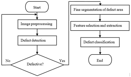
Figure 1.
Flow chart of the algorithm.
- Step 1:
- Perform image preprocessing, filtering, and correction.
- Step 2:
- Perform defect detection, position the inspection object, and detect whether it has defects.
- Step 3:
- Perform fine segmentation of the defect area. If a defect is detected, the defect area will be precisely segmented, and the detailed features of the defect area will be retained to the greatest extent possible.
- Step 4:
- Perform feature selection. According to the sample data and dimensionality reduction goals, use the designed feature selection algorithm to select a feature combination with good classification performance from the feature pool.
- Step 5:
- Perform defect classification. Based on the selected features, use pattern recognition technology to identify the type of defect.
3.1. Image Preprocessing
The basic principle of this step of the algorithm is to read the image to be inspected, first filtering the image to make the edges of the image smoother and more continuous, then performing edge detection on the image to detect the upper edge of the bearing, and finally adjusting the image according to the y-coordinate difference in edge pixel coordinates. The corresponding column is adjusted to position the edge line at the same y coordinate to correct the distortion. The goal of the image correction is to correct the distortion of the image collected by the line array camera to restore the original characteristics of the image. The specific algorithm steps are as follows:
- Step 1:
- Perform a 3 × 3 median value filter on the distorted image.
- Step 2:
- Detect an obvious edge of the bearing ring with the Canny operator to serve as a reference line.
- Step 3:
- Using the starting point of the reference line as the reference point, calculate the y-coordinate difference between each pixel point of the edge and the reference point in the y-direction.
- Step 4:
- Keeping the reference point unchanged, cyclically move the remaining columns of pixels according to the magnitude and sign of the difference to obtain a corrected image.
For the images of the inner and outer sides of the bearing ring, a flute of the bearing may be chosen as the reference line, as lines marked by a star shown in Figure 2a,c. Perform the correction according to the above algorithm to obtain the corrected results, shown in Figure 2b,d.
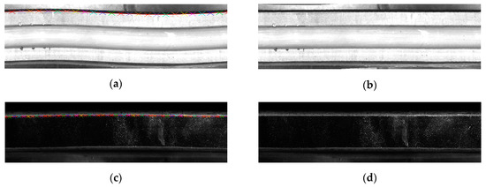
Figure 2.
Comparison of side images before and after correction: (a) inner side image before correction; (b) inner side image after correction; (c) outer side image before correction; (d) outer side image after correction.
3.2. Defect Detection
Defect detection is divided into two steps. Locate the position of the bearing image in the whole image and separate it from the background to automatically obtain the ROI. Then, use the defect detection algorithm to determine whether the bearing in the ROI is defective.
3.2.1. Region-of-Interest (ROI) Extraction
The bearing is placed flat on the turntable, the linear array camera is parallel to the axis of the bearing, the turntable rotates at a constant speed, and the linear array camera scans the outer ring of the bearing synchronously. The acquired bearing image is divided into three areas: the bottom turntable area, the central bearing area, and the upper background area. As the three areas are distributed along the y-axis, they are well aligned in the x-axis, the gray level of the black background in the upper part is low, and the gray level of the turntable image in the bottom part is high, where the features are more pronounced and relatively stable, and it is easy to detect them by using the feature region localization algorithm. The design algorithm goes as follows:
- Step 1:
- Perform a mean value filter on the image.
- Step 2:
- Convert the filtered image into a binary image.
- Step 3:
- Based on local features of the binary image, select the dark background portion of the bearing image.
- Step 4:
- Using the smallest circumscribed rectangle, determine the coordinate of the center of the dark background.
- Step 5:
- Based on the size of the bearing image at the center, establish a rectangular model for the central bearing region.
- Step 6:
- Using the position information of the dark background region and its relative position to the central bearing image, locate the rectangular model of the bearing and obtain the ROI region.
Figure 3 shows the processing procedure on a ground waste sample according to the steps described above.
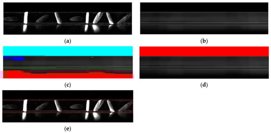
Figure 3.
Feature location region-of-interest (ROI) extraction process: (a) original image; (b) filtered image; (c) region after conversion into binary; (d) dark background region; (e) ROI extraction result.
3.2.2. Defect Detection Algorithm
The structural characteristics of the bearing determine the high level of gray-scale consistency of the images along the x-axis, but the appearance of defects often disrupts this consistency. Based on this, we designed the following algorithm:
- Step 1:
- Perform a Gaussian filter on the image to eliminate the influence of noise, such as fingerprints on the bearing surface, and generate a Gaussian-filtered image.
- Step 2:
- Calculate the average value of each row of pixels along the x-axis to generate an average filtered image.
- Step 3:
- Form a difference value image using the difference between the Gaussian-filtered image and the mean filtered image.
- Step 4:
- Identify the defective region, which is the region in the difference image where the amplitude is greater than the preset threshold.
Figure 4 shows the detection results of images with a certain level of noise.
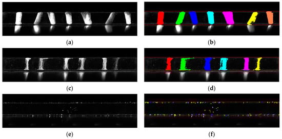
Figure 4.
Test results obtained using image detection algorithm for different defects: (a) original image of over-grinding; (b) detection result of over-grinding; (c) original image of the scratch defect; (d) detection results of the scratch defect; (e) original image of the bruise defect; (f) detection results of the bruise defect.
3.3. Precision Segmentation of Defect Region
Gaussian filter processing is used in the defect detection process. The process eliminates noise but also blurs the boundary of the defect, reduces the accuracy of the segmentation of the defect region, and can even affect the classification of the defect. Therefore, it is necessary to perform accurate segmentation of the region obtained above.
To address this situation based on previous research, we proposed a local multiple neural network (Lc-MNN) image segmentation algorithm for extracting the features with the wavelet transform to further process the initial segmented images to improve the accuracy of segmentation. The application of the algorithm was carried out based on the initially segmented results. The algorithm comprises three steps: feature extraction with the wavelet transform, region division with Lc-MNN, and classification and post-processing with Lc-MNN. The steps are as follows.
- Step 1:
- Wavelet transform feature extraction: perform a three-layer wavelet transform on the original image to obtain a series of high-frequency and low-frequency images stacked in a pyramid structure (as shown in Figure 5a). These images are expanded to the size of the original image by nearest-neighbor interpolation (as shown in Figure 5b), together with the original image. Each pixel location is characterized by an 11-dimensional feature to form a feature vector for each pixel.
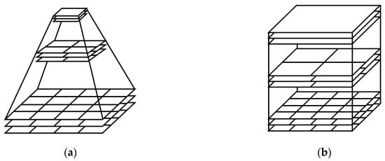 Figure 5. Multi-scale image feature structure: (a) pyramid structure of the images; (b) cuboid structure of the images.
 - Step 2:
- Lc-MNN region division: first, perform morphological processing of the image using the boundary of the initial segmentation to form an overall to-be-classified region, a target sample region, and a background sample region centered on the boundary. Then, fit the boundary curve with an N-sided polygon and generate N symmetric rectangles centered on the N sides, with each rectangle representing a neural-network region. Finally, each rectangle is intersected with the overall to-be-classified region, the target sample region, and the background sample region to obtain the to-be-classified region, the target sample region, and the background sample region of each neural-network region.
- Step 3:
- Lc-MNN classification and post-processing. After the above two steps, the training sample and to-be-classified pixel in the i-th neural network region can be represented by 11-dimensional features. Use training samples to train the neural network to obtain the neural network classifier, and then the feature vector of the pixel to be classified is input into the classifier to obtain the classification result of whether each pixel belongs to the target region. This process may produce unconnected areas or holes in the area, but these artifacts may be eliminated through regional operations to obtain the segmentation results.
The framework of the algorithm is shown in Figure 6.
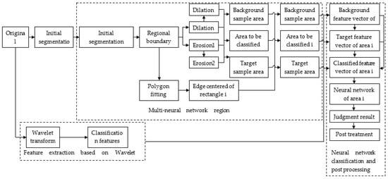
Figure 6.
The framework of the multi-neural network segmentation algorithm.
3.4. Feature Selection and Extraction
To accurately identify the type of bearing surface defects, it is necessary to select efficient classification features. We proposed the comprehensive use of a practical algorithm that combines scalar feature selection [25,26,27,28,29,30,31], correlation analysis [27,28], and vector selection [29,30], abbreviated as the SCV algorithm.
The SCV feature selection algorithm is mainly divided into the following four steps:
- Step 1:
- Establish a feature pool. Collect as many features of the classified object as possible and combine them into a set of candidate features.
- Step 2:
- Perform data acquisition and processing. Complete the conversion of a sample from an image to a normalized feature vector through the steps of image acquisition, image processing, and feature calculation.
- Step 3:
- Set a target of dimension reduction. Make a comprehensive determination of the number of features to be used for classification based on the dimension of features in the feature pool, peak phenomenon, and number of training samples.
- Step 4:
- Perform SCV feature selection. Based on the sample data and the dimensionality reduction target, use the designed feature selection algorithm to select a set of features from the feature pool with good classification performance. First, rank the features by their classification performance, from good to poor, based on the separability criterion to realize the conversion from feature pool to feature vector . Second, perform correlation analysis between features to eliminate strongly correlated features and reduce the dimensionality of the feature vector from to . Then, carry out a scalar feature selection on , i.e., select only the first features from to form a new feature vector to complete the second dimensionality reduction. Finally, perform a vector feature selection on to select the optimal classification set of features from to obtain the final classification feature vector .
According to the above algorithm design, we established a feature selection criterion based on the correlation coefficient. The specific algorithm uses the Fisher criterion for scalar feature selection and as the selection criterion for the feature vector.
According to the algorithm procedure, assume that a feature pool, , has been established, a standardized training sample set, , has been obtained, and a dimensionality reduction goal, , has been established. Here, the feature pool has d features, expressed as . Moreover, has types (), designated as , respectively, with each type having samples, for a total of training samples. The aim of is to choose features as the final classification features from the feature pool of d features. The specific steps are:
- Step 1:
- Perform Fisher discrimination ratio (FDR) feature sequence. The features in the feature pool exist in an aggregate form. For the ease of representation and computation, all features need to be sequenced in a certain order to form a feature vector. They may be ordered according to the FDR in descending order. FDR is used to characterize the separability of a single feature. The larger the FDR value, the better the separability of the feature.
For any feature in the feature pool, its FDR value [46] is
Here, is the k-th sample of the type represented by the feature, is the average value of feature of type , and is the variance of feature of type .
By carrying out the above calculation for all features in X, one can obtain the FDR values for all the features. By rearranging the FDR values according to their magnitude, one can obtain the feature vector .
- Step 2:
- Perform correlation feature selection. Arrange features xl of all the samples in training sample set T according to the sequence to form vector . As each sample has d features, it is possible to generate d vectors of this kind. The correlation coefficient between any two vectors and is:
Select the features for their correlation coefficient based on the sequence of the features and their correlation coefficient. First, eliminate features with correlation coefficients with x1 that are greater than the preset threshold. Then, use the remaining features to eliminate features with correlation coefficients that are greater than the threshold, until the last feature is reached. Through this screening, one obtains a feature vector x(d1) that has a low correlation with the various features, thus accomplishing the first dimensionality reduction.
- Step 3:
- Perform FDR feature selection. After screening according to the correlation coefficient, the remaining features not only retain the classification information of the original features but also greatly reduce the correlation between the features, hence satisfying the basic conditions of scalar feature selection. Moreover, as the features have already been sorted by FDR, so the first d2 features may be chosen directly to form a new feature vector to achieve the second dimensionality reduction.
- Step 4:
- Perform vector feature selection. After the above two-dimensionality reduction operations, the number of features is sufficiently reduced for the normal use of the feature vector selection method. For example, if 10 of the 60 features are directly selected as the classification features, one must compute the criterion value times, which is too large to implement. If there are 24 features after the two-dimensionality reductions, then selecting 10 features out of 24 will only require computing the criterion value times, which is four orders of magnitude smaller. The feature vector selection is implemented in two steps:
(1) Select any features from the features in as a set and calculate the value of all combinations, namely, which is as follows [24]:
where is the feature vector of the k-th sample of the type.
(2) Select the combination that maximizes the value, realize the third dimensionality reduction, and obtain the final classification feature .
3.5. Defect Classification
The classification of bearing surface defects is completed by the classifier, and an error back-propagation training algorithm is used to complete the non-linear mapping from the input signal to the output mode. The steps are as follows:
- Step 1:
- Choose an initial value of the weight coefficient.
- Step 2:
- Input a sample and its expected output .
- Step 3:
- Calculate the actual output .
- Step 4:
- Backward-adjust the weights from the output layer forward, layer by layer, using the adjustment formula [36]:
Here, represents all the nodes on the layer before node . To improve the convergence, the following formula may be used for weight update correction:
Here, 0 < < 1; that is, a subsequent adjustment of the weight value takes into account the last update of weight value.
- Step 5:
- Go back to Step 3 and repeat the execution until the error requirements are met.
4. Experiment
4.1. Experimental Design
The test object of this paper is the outer ring of 6204 deep groove ball bearings (6204 bearings, outer diameter 47 mm, inner diameter 20 mm, height 14 mm, weight 0.11 kg, Cr: 15.8KN, Cor: 7.88KN, DW: 9.525 mm, Z: 7). Based on the experimental requirements, the detection system consisted of a lower machine and the main computer. The lower machine included a programmable logic controller (PLC), DALSA linear array camera, linear light source, and self-made loading and unloading control mechanism. The main computer was a Dell Precision T3630 graphics workstation (Intel i7-10700K, 8-core, 16 lines, 3.8 G, 32 G memory, and a Windows operating system), The programming languages used were MATLAB and C++. The lower machine was responsible for digital IO (input and output) and motion control, and the main computer was responsible for image acquisition, image processing, and the resulting output. In operation, the bearing to be inspected was automatically placed on the turntable and centered, the image acquisition switch was turned on, the encoder drove the turntable to rotate at a constant preset speed, the line light source was turned on, and the line array camera automatically-collected images and sent them to the main computer, which performed various operations and processing on the image, positioned the image under test, detected and identified the inspected object, and generated motion control decisions based on the processing results.
In the test of model 6204 bearing, three types of commonly occurring surface defects in the machining process of the outer ring, namely over-grinding, scratches, and bruises, were selected as identification objects. A total of 900 defect samples were collected, with 300 of each type of defect. Some examples of the defects are shown in Figure 7.
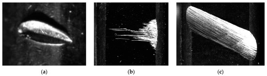
Figure 7.
Examples of the defect images: (a) original image of the bruise defect; (b) original image of the scratch defect; (c) original image of over-grinding.
4.2. Segmentation Experiment
4.2.1. Experiment Process
This experiment was to verify that the Lc-MNN algorithm can effectively improve the accuracy of segmentation for images of bearing surface defects. The threshold algorithm has the advantages of simple calculation, high operating efficiency, and strong versatility, and is widely used. It was used here as a comparison algorithm for the Lc-MNN algorithm. During the experiment, the maximum error acceptance rate in each network training was set to 0.001. Figure 8 shows the original image to be segmented, Figure 9 shows the standard image of manual segmentation, Figure 10 shows the multi-scale feature of the extracted original image, and Figure 11 shows the process and result of the multi-region division. The small region in Figure 11d starts from the small area in the upper right-hand corner and is labeled a, b, and c in a clockwise direction.
Figure 8.
Image to be segmented.
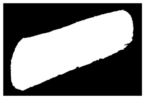
Figure 9.
Standard segmented image.
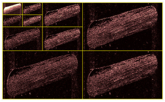
Figure 10.
Multi-scale feature images.
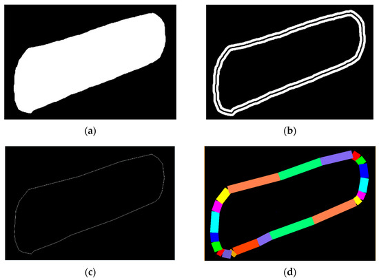
Figure 11.
Region segmentation process with multi-neural network: (a) initial segmented region; (b) morphological processing result; (c) boundary polygon; (d) multi-neural network region.
To illustrate the classification process of each small region, the segmentation process of a small area, a, in Figure 11d was chosen for the detailed description. Figure 12a is an image of the region to be classified, Figure 12b is an image of the background region, and Figure 12c is an image of the target area. The neural network was established with MATLAB, and the corresponding training was carried out. Pixels in the region to be classified were classified using the trained neural network to obtain pixels belonging to the target region, as shown in Figure 12d. By performing this operation on all small regions, we obtained the target pixels in the region to be classified. By combining all the target pixels with the original region, the final segmentation result was obtained.
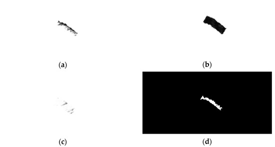
Figure 12.
Segmentation process of a small region, (a) small region a to be segmented; (b) background region in the small region a; (c) target region in the small region a; (d) segmentation result of the small region.
4.2.2. Discussion of Results
This experiment used the pixel number error criterion, which is defined as follows [32]:
where is the probability that the object is incorrectly classified as the background, is the probability that the background is incorrectly classified as the object, and and represent the a priori probability of the proportion of the object and the background in the image, respectively. The smaller PE was, the fewer pixels were misclassified, and the higher the accuracy of image segmentation. Figure 13 shows the results obtained from the Lc-MNN segmentation algorithm and those obtained from the threshold segmentation algorithm, as well as the difference from the standard image.
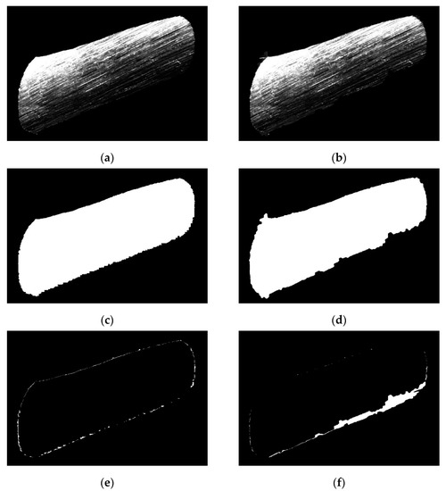
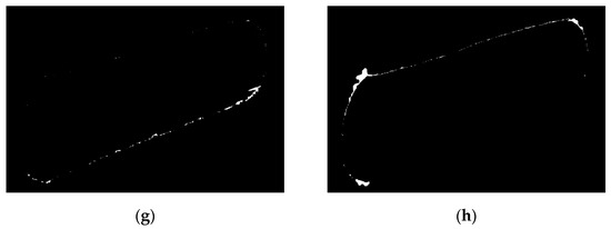
Figure 13.
Comparison of segmentation results between the local multi-neural network (Lc-MNN) algorithm and the threshold algorithm: (a) Lc-MNN algorithm segmentation result; (b) threshold algorithm segmentation result; (c) Lc-MNN algorithm segmented region; (d) threshold algorithm segmented region; (e) Lc-MNN algorithm ; (f) threshold algorithm ; (g) Lc-MNN algorithm ; (h) threshold algorithm .
The calculated values of the two methods are listed in Table 1.

Table 1.
Lc-MNN segmentation algorithm and threshold segmentation algorithm PE values.
Table 1 lists the PE values computed from the two algorithms. As the results in Table 1 show, the segmented image using the Lc-MNN algorithm proposed in this work showed considerable improvement over the threshold segmentation algorithm both in terms of background misclassification and object misclassification. The PE value based on Lc-MNN algorithm was 75% less than that based on the threshold segmentation algorithm. Thus, the segmentation accuracy improved substantially, and the expected target was reached.
4.3. Defect Classification Experiment
4.3.1. Experimental Process
Three sets of features were chosen using the random selection algorithm, and one set of features was extracted with the scalar feature selection algorithm and the algorithm proposed in this work, for a total of five sets of experiments. Then, 100 samples were randomly chosen from each defect category as training samples, each sample was assigned an ID number, and the remaining 600 samples were each assigned an ID number and used as test samples. The 57 features listed in Table 1 were treated as original features. The target for dimensionality reduction was set to 10 features chosen from 60 features. Images were collected with a linear camera in a scanning mode, the defective regions were segmented using the dynamic threshold segmentation algorithm, and a component whitening algorithm was used for normalization processing. Based on 300 training samples, features were selected using the random extraction algorithm, the scalar feature selection algorithm, and the algorithm from this paper. The neural network structure was determined according to the dimension of the input features, categories of the output, and other factors. The selected features were then used to train multiple neural networks with the same structure, and the trained neural networks were used to identify the test samples. The identification rate of each method was obtained and used in the comparison study.
4.3.2. Discussion of Results
The test results are shown in Table 2. The table shows that the identification rates were low and quite unstable for the three groups of random algorithm tests; the highest identification rate reached was 82.2%, and the lowest identification rate was only 19.0%. The scalar feature selection experiment conducted with the FDR criterion did not achieve good results; the identification rate was only 66.7%. Further analysis revealed that the classification error was mainly misidentifying all 200 over-grinding defects like scratches, but the other two categories were both identified correctly. This result confirmed a flaw of the algorithm itself: the individually selected features have good separability, but there may be a strong correlation between the features, which reduced the overall classification ability of the feature combination and led to misidentification. In comparison, the algorithm of this paper achieved good results. Among the 600 test samples, only three were misidentified: The scratch defect of #402 was misidentified as a bruise, and the scratch defects of #492 and #600 were misidentified as over-grinding, as shown in Figure 14. The remaining samples were all correctly identified, and the identification rate was as high as 99.5%, reaching the expected goal. Table 3 shows the rest of the experimental data, including the five sets of data for each type of defect and the sample data (marked in gray) that were incorrectly identified.
Table 2.
Comparison of the identification rate of each feature selection algorithm.
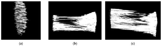
Figure 14.
Misclassified sample: (a) scratch defect, #402; (b) scratch defect, #492; (c) scratch defect, #600.
Table 3.
Input and output values of the back-propagation neural network of some of the samples detected by the proposed algorithm.
5. Conclusions
We proposed a method for detecting and classifying bearing surface defects. The main content and innovations of this work were as follows:
- (1)
- A local multi-neural network algorithm (Lc-MNN) for image segmentation is proposed; the method includes three stages: wavelet feature extraction, Lc-MNN region division, and Lc-MNN classification. The classification features are obtained by expanding the images at the various layers of the wavelet transform. The Lc-MNN regional division divides the area near the initial segmentation boundary into a region of training samples and a region of samples to be classified, and a polygon fitting algorithm is used to divide the above area into multiple local areas. The Lc-MNN classification process classifies the pixels in each region to be classified using the neural networks within the region to discriminate target pixels and background pixels. After combining the target pixels obtained and performing some post-processing, one obtains the segmentation results of higher precision. The experiments indicated that the proposed algorithm can effectively improve the accuracy of segmentation, which is one of the innovations of the algorithm.
- (2)
- We proposed an SCV algorithm for feature selection. The algorithm first removes similar features through correlation analysis, further screens the results using the scalar feature selection algorithm, and finally uses the feature vector selection algorithm to select the final classification features. The experiments indicated that the SCV algorithm can effectively improve the classification accuracy and avoid large-scale computation, which is another innovation of the algorithm developed in this research.
Through comparative experiments, and with the two improvements described above, we found that the identification rate reached 99.5% and large-scale calculations could be avoided in experiments on 600 test samples with three types of defect. In future work, we hope to add more sample images to the bearing surface defect data and improve the network structure for defect feature extraction. We also plan to study defect detection and classification and identification techniques based on deep learning and the automatic iteration of internet-based classifiers.
Author Contributions
M.L. and C.-L.C. made substantial contributions to the conception and design. M.L. was involved in drafting the manuscript. M.L. acquired data and analysis and conducted the interpretation of the data. The critically important intellectual content of this manuscript was revised by C.-L.C. All authors have read and agreed to the published version of the manuscript.
Funding
This research was supported by the National Social Science Fund of China (20BGL141).
Informed Consent Statement
This study is only based on theoretical basic research. It does not involve human subjects.
Data Availability Statement
The data used to support the findings of this study are available from the corresponding author upon request.
Conflicts of Interest
The authors declare no conflict of interest.
Abbreviations
| ROI | Region of Interest |
| LBF | Local Binary Fitting |
| MLoG | Modified Lapalcian-of-Gaussian |
| BP | Back Propagation |
| SVM-RFE | Support Vector Machine Recursive Feature Elimination |
| PCA | Principal Component Analysis |
| LLE | Locally linear Embedding |
| Lc-MNN | Local Multiple Neural Network Algorithm |
| SCV | Scalar selection, Correlation analysis, Vector selection |
| FDR | Fisher Discrimination Ratio |
| PLC | Programmable Logic Controller |
References
- Shen, H.; Li, S.; Gu, D.; Chang, H. Bearing defect inspection based on machine vision. Measurement 2012, 45, 719–733. [Google Scholar] [CrossRef]
- Malamas, E.N.; Petrakis, E.G.M.; Zervakis, M.; Petit, L.; Legat, J.-D. A survey on industrial vision systems, applications, and tools. Image Vis. Comput. 2003, 21, 171–188. [Google Scholar] [CrossRef]
- Hemmati, F.; Miraskari, M.; Gadala, M.S. Application of wavelet packet transform in roller bearing fault detection and life estimation. J. Phys. Conf. Ser. 2018, 1074, 012142. [Google Scholar] [CrossRef]
- Bastami, A.R.; Vahid, S. Estimating the size of naturally generated defects in the outer ring and roller of a tapered roller bearing based on autoregressive model combined with envelope analysis and discrete wavelet transform. Measurement 2020, 159, 107767. [Google Scholar] [CrossRef]
- Sobie, C.; Freitas, C.; Nicolai, M. Simulation-driven machine learning: Bearing fault classification. Mech. Syst. Signal Process. 2018, 99, 403–419. [Google Scholar] [CrossRef]
- Zheng, H.; Kong, L.X.; Nahavandi, S. Automatic inspection of metallic surface defects using genetic algorithms. J. Mater. Process. Technol. 2002, 125, 427–433. [Google Scholar] [CrossRef]
- Pernkopf, F.; O’Leary, P. Image acquisition techniques for automatic visual inspection of metallic surfaces. NDT E Int. 2003, 36, 609–617. [Google Scholar] [CrossRef]
- Phung, V.T.; Pacas, M. Senseless harmonic speed control and detection of bearing faults in repetitive mechanical systems. In Proceedings of the IEEE 3rd International Future Energy Electronics Conference and ECCE Asia, Kaohsiung, Taiwan, 3–7 June 2017; pp. 1646–1651. [Google Scholar]
- Kunakornvong, P.; Sooraksa, P. A Practical Low-Cost Machine Vision Sensor System for Defect Classification on Air Bearing Surfaces. Sens. Mater. 2017, 29, 629–644. [Google Scholar]
- Chen, Y.J.; Tsai, J.C.; Hsu, Y.C. A real-time surface inspection system for precision steel balls based on machine vision. Meas. Sci. Technol. 2016, 27, 74–100. [Google Scholar] [CrossRef]
- Mikołajczyk, T.; Nowicki, K.; Kłodowski, A.; Pimenov, D.Y. Neural network approach for automatic image analysis of cutting edge wear. Mech. Syst. Signal Process. 2017, 88, 100–110. [Google Scholar] [CrossRef]
- Van, M.; Kang, H.J. Bearing Defect Classification Based on Individual Wavelet Local Fisher Discriminant Analysis with Particle Swarm Optimization. IEEE Trans. Ind. Inform. 2017, 12, 124–135. [Google Scholar] [CrossRef]
- Mikołajczyk, T.; Nowicki, K.; Bustillo, A.; Pimenov, D.Y. Predicting tool life in turning operations using neural networks and image processing. Mech. Syst. Signal Process. 2018, 104, 503–513. [Google Scholar] [CrossRef]
- Guo, Y.; Jiao, L.; Wang, S.; Wang, S.; Liu, F. Fuzzy Sparse Autoencoder Framework for Single Image per Person Face Recognition. IEEE Trans. Cybern. 2018, 48, 2402–2415. [Google Scholar] [CrossRef] [PubMed]
- Chen, H.; Zhang, B.; Li, M.; Zhang, C. Surface defect detection of bearing roller based on image optical flow. Chin. J. Sci. Instrum. 2018, 39, 198–206. [Google Scholar]
- Ciobanu, R.; Rizescu, D.; Rizescu, C. Automatic Sorting Machine Based on Vision Inspection. Int. J. Model. Optim. 2017, 7, 286–290. [Google Scholar]
- Riggio, M.; Sandak, J.; Franke, S. Application of imaging techniques for detection of defects, damage and decay in timber structures onsite. Constr. Build. Mater. 2015, 101, 1241–1252. [Google Scholar] [CrossRef]
- Martínez, S.S.; Vázquez, C.O.; García, J.G.; Ortega, J.G. Quality inspection of machined metal parts using an image fusion technique. Measurement 2017, 111, 374–383. [Google Scholar] [CrossRef]
- Huang, D.; Liao, S.; Sunny, A.I.; Yu, S. A novel automatic surface scratch defect detection for fluid-conveying tube of Coriolis mass flow-meter based on 2D-direction filter. Measurement 2018, 126, 332–341. [Google Scholar] [CrossRef]
- Chondronasios, A.; Popov, I.; Jordanov, I. Feature selection for surface defect classification of extruded aluminum profiles. Int. J. Adv. Manuf. Technol. 2015, 83, 33–41. [Google Scholar] [CrossRef]
- Tao, X.; Zhang, D.; Ma, W.; Liu, X.; Xu, D. Automatic Metallic Surface Defect Detection and Recognition with Convolutional Neural Networks. Appl. Sci. 2018, 8, 1575. [Google Scholar] [CrossRef]
- Lin, J.; Yao, Y.; Ma, L.; Wang, Y. Detection of a casting defect tracked by deep convolution neural network. Int. J. Adv. Manuf. Technol. 2018, 97, 573–581. [Google Scholar] [CrossRef]
- Yu, W.; Yanjie, L. An intelligent machine vision system for detecting surface defects on packing boxes based on support vector machine. Meas. Control 2019, 52, 1102–1110. [Google Scholar]
- Labudzki, R.; Legutko, S.; Raos, P. The essence and applications of machine vision. Teh. Tech. Gaz. 2019, 21, 903–909. [Google Scholar]
- Kittler, J.; Illingworth, J. Minimum error thresholding. Pattern Recognit. 1986, 19, 41–47. [Google Scholar] [CrossRef]
- Wong, A.K.; Sahoo, P.K. A gray-level threshold selection method based on maximum entropy principle. IEEE Trans. Syst. Man Cybern. 1989, 19, 866–871. [Google Scholar] [CrossRef]
- Tsai, W.-H. Moment-preserving thresholding: A new approach. Comput. Vis. Graph. Image Process. 1985, 29, 377–393. [Google Scholar] [CrossRef]
- Chen, P.C.; Pavlidis, T. Segmentation by texture using a co-occurrence matrix and a split-and-merge algorithm. Comput. Graph. Image Process. 1979, 10, 172–182. [Google Scholar] [CrossRef]
- Hojjatoleslami, S.; Kittler, J. Region growing: A new approach. IEEE Trans. Image Process. 1998, 7, 1079–1084. [Google Scholar] [CrossRef]
- Gao, Y.; Mas, J.F.; Kerle, N.; Navarrete Pacheco, J.A. Optimal region growing segmentation and ts effect on classification accuracy. Int. J. Remote Sens. 2011, 32, 3747–3763. [Google Scholar] [CrossRef]
- Biswas, S.; Hazra, R. Active contours driven by modified LoG energy term and optimised penalty term for image segmentation. IET Image Process. 2020, 14, 3232–3242. [Google Scholar] [CrossRef]
- Tarkhaneh, O.; Shen, H. An adaptive differential evolution algorithm to optimal multi-level thresholding for MRI brain image segmentation. Expert Syst. Appl. 2019, 138, 112820. [Google Scholar] [CrossRef]
- Abd Elaziz, M.; Bhattacharyya, S.; Lu, S. Swarm selection method for multilevel thresholding image segmentation. Expert Syst. Appl. 2019, 138, 112818. [Google Scholar] [CrossRef]
- Alroobaea, R.; Rubaiee, S.; Bourouis, S.; Bouguila, N.; Alsufyani, A. Bayesian inference framework for bounded generalized Gaussian-based mixture model and its application to biomedical images classification. Int. J. Imaging Syst. Technol. 2019, 30, 18–30. [Google Scholar] [CrossRef]
- Narisetti, N.; Henke, M.; Seiler, C.; Shi, R.; Junker, A.; Altmann, T.; Gladilin, E. Semi-automated Root Image Analysis (saRIA). Sci. Rep. 2019, 9, 19674. [Google Scholar] [CrossRef] [PubMed]
- Zhang, Y.; Xu, C.; Li, C.; Yu, H.; Cao, J. Wood defect detection method with PCA feature fusion and compressed sensing. J. For. Res. 2015, 26, 745–751. [Google Scholar] [CrossRef]
- Lu, M.; Mou, Y. Bearing Defect Classification Algorithm Based on Autoencoder Neural Network. Adv. Civ. Eng. 2020, 12. [Google Scholar] [CrossRef]
- Yan, K.; Zhang, D. Feature selection and analysis on correlated gas sensor data with recursive feature elimination. Sens. Actuators B Chem. 2015, 212, 353–363. [Google Scholar] [CrossRef]
- Lu, M.; Chen, L. Efficient Object Detection Algorithm in Kitchen Appliance Scene Images Based on Deep Learning. Math. Probl. Eng. 2020, 12. [Google Scholar] [CrossRef]
- Spetale, F.E.; Bulacio, P.; Guillaume, S.; Murillo, J.; Tapia, E. A spectral envelope approach towards effective SVM-RFE on infrared data. Pattern Recognit. Lett. 2016, 71, 59–65. [Google Scholar] [CrossRef]
- Ding, X.; Yang, Y.; Stein, E.A.; Ross, T.J. Multivariate classification of smokers and nonsmokers using SVM-RFE on structural MRI images. Hum. Brain Mapp. 2015, 36, 4869–4879. [Google Scholar] [CrossRef]
- Zhao, J.; Jia, M. Feature extraction with global-locally preserving projections based on curvelet transform. In Electronics, Electrical Engineering, and Information Science, Proceedings of the 2015 International Conference on Electronics, Electrical Engineering, and Information Science (EEEIS2015), Guangzhou, China, 7–9 August 2015; World Scientific: Singapore, 2015. [Google Scholar]
- Yildiz, K.; Buldu, A.; Demetgul, M. A thermal-based defect classification method in textile fabrics with K-nearest neighbor algorithm. J. Ind. Text. 2016, 45, 780–795. [Google Scholar] [CrossRef]
- Dubey, S.R.; Dixit, P.; Singh, N.; Gupta, J.P. Infected fruit part detection using K-means clustering segmentation technique. IJIMAI 2013, 2, 65–72. [Google Scholar] [CrossRef]
- Mu, W.; Gao, J.; Jiang, H.; Wang, Z.; Chen, F.; Dang, C. Automatic classification approach to weld defects based on PCA and SVM. Insight-Non-Destr. Test. Cond. Monit. 2013, 55, 535–539. [Google Scholar] [CrossRef]
- Muhammad, G. Date fruits classification using texture descriptors and shape-size features. Eng. Appl. Artif. Intell. 2015, 37, 361–367. [Google Scholar] [CrossRef]


Publisher’s Note: MDPI stays neutral with regard to jurisdictional claims in published maps and institutional affiliations. |
© 2021 by the authors. Licensee MDPI, Basel, Switzerland. This article is an open access article distributed under the terms and conditions of the Creative Commons Attribution (CC BY) license (http://creativecommons.org/licenses/by/4.0/).