
Performance Evaluation of Hybrid WOA-SVR and HHO-SVR Models with Various Kernels to Predict Factor of Safety for Circular Failure Slope


Abstract
:1. Introduction
2. Methodology
2.1. Support Vector Regression (SVR)
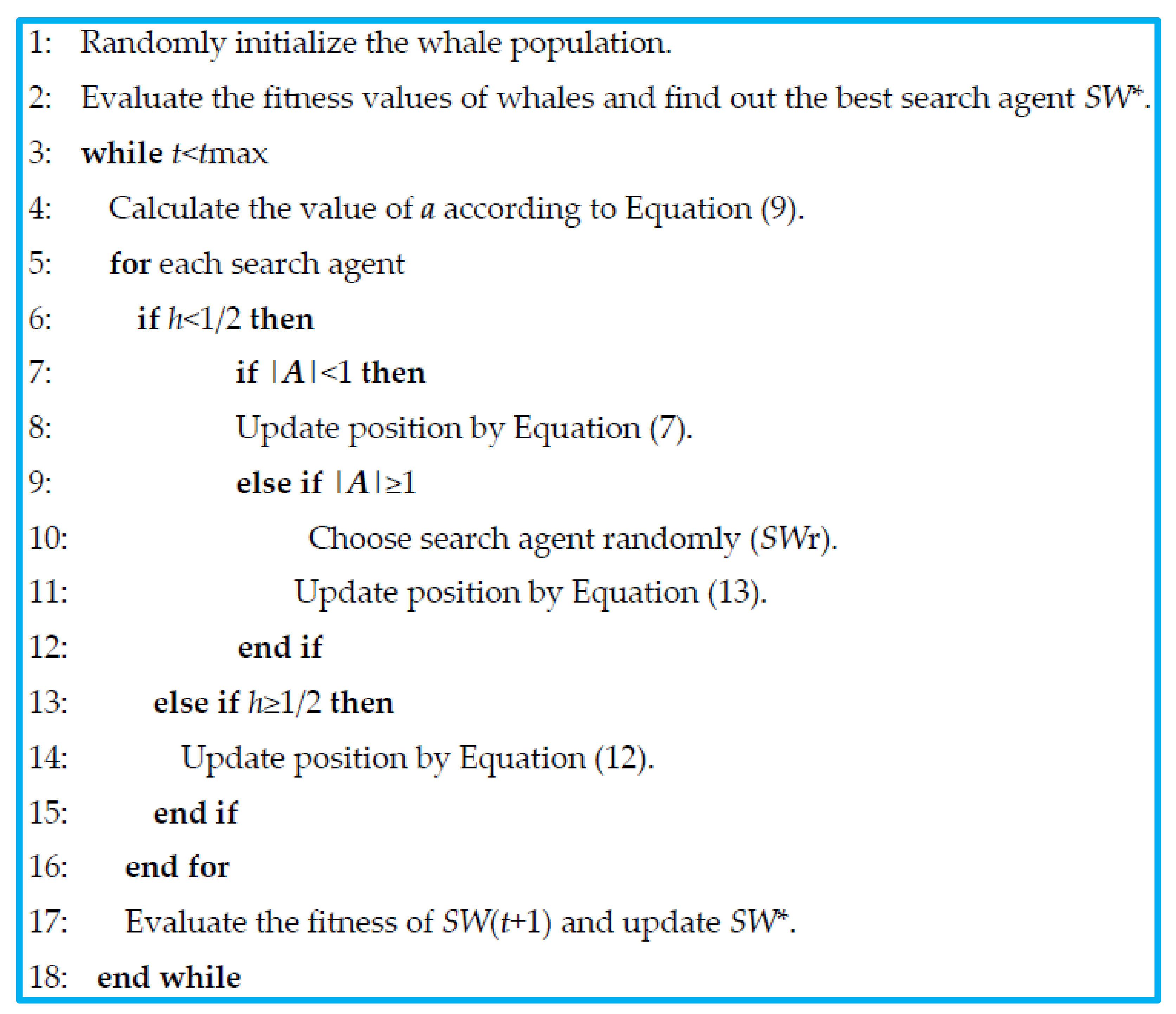
2.2. Whale Optimization Algorithm (WOA)
2.3. Harris Hawks Optimization (HHO)
2.4. Evaluation
3. Results and Discussion
3.1. Data Preparation
3.2. Study Steps
3.3. Simulation
3.4. Model Validation
3.5. Optimization
4. Discussion
5. Conclusions
Author Contributions
Funding
Institutional Review Board Statement
Informed Consent Statement
Data Availability Statement
Conflicts of Interest
References
- Zhou, J.; Li, E.; Yang, S.; Wang, M.; Shi, X.; Yao, S.; Mitri, H.S. Slope stability prediction for circular mode failure using gradient boosting machine approach based on an updated database of case histories. Saf. Sci. 2019, 118, 505–518. [Google Scholar] [CrossRef]
- Tan, Ö. Investigation of soil parameters affecting the stability of homogeneous slopes using the Taguchi method. Eurasian Soil Sci. 2006, 39, 1248–1254. [Google Scholar] [CrossRef]
- Erzin, Y.; Cetin, T. The prediction of the critical factor of safety of homogeneous finite slopes using neural networks and multiple regressions. Comput. Geosci. 2013, 51, 305–313. [Google Scholar] [CrossRef]
- Nash, D. A comparative review of limit equilibrium methods of stability analysis. Slope Stab. 1987, 10008435061, 11–75. [Google Scholar]
- Duncan, J.M. State of the Art: Limit Equilibrium and Finite-Element Analysis of Slopes. J. Geotech. Eng. 1996, 122, 577–596. [Google Scholar] [CrossRef]
- Zucca, M.; Valente, M. On the limitations of decoupled approach for the seismic behaviour evaluation of shallow multi-propped underground structures embedded in granular soils. Eng. Struct. 2020, 211, 110497. [Google Scholar] [CrossRef]
- Su, Z.; Shao, L. A three-dimensional slope stability analysis method based on finite element method stress analysis. Eng. Geol. 2021, 280, 105910. [Google Scholar] [CrossRef]
- Liang, H.; Zhang, H. Identification of slope stability based on the contrast of BP neural network and SVM. In Proceedings of the 3rd International Conference on Computer Science and Information Technology, Chengdu, China, 9–11 July 2010; Volume 9, pp. 347–350. [Google Scholar]
- Shahin, M.A.; Jaksa, M.B.; Maier, H.R. State of the art of artificial neural networks in geotechnical engineering. Electron. J. Geotech. Eng. 2008, 8, 1–26. [Google Scholar]
- Zhou, J.; Li, C.; Arslan, C.A.; Hasanipanah, M.; Amnieh, H.B. Performance evaluation of hybrid FFA-ANFIS and GA-ANFIS models to predict particle size distribution of a muck-pile after blasting. Eng. Comput. 2021, 37, 265–274. [Google Scholar] [CrossRef]
- Mohamad, E.T.; Koopialipoor, M.; Murlidhar, B.R.; Rashiddel, A.; Hedayat, A.; Armaghani, D.J. A new hybrid method for predicting ripping production in different weathering zones through in situ tests. Measurement 2019, 147, 106826. [Google Scholar] [CrossRef]
- Sun, L.; Koopialipoor, M.; Armaghani, D.J.; Tarinejad, R.; Tahir, M.M. Applying a meta-heuristic algorithm to predict and optimize compressive strength of concrete samples. Eng. Comput. 2019, 1–13. [Google Scholar] [CrossRef]
- Armaghani, D.J.; Hatzigeorgiou, G.D.; Karamani, C.; Skentou, A.; Zoumpoulaki, I.; Asteris, P.G. Soft computing-based techniques for concrete beams shear strength. Procedia Struct. Integr. 2019, 17, 924–933. [Google Scholar] [CrossRef]
- Asteris, P.G.; Apostolopoulou, M.; Skentou, A.D.; Moropoulou, A. Application of artificial neural networks for the prediction of the compressive strength of cement-based mortars. Comput. Concr. 2019, 24, 329–345. [Google Scholar]
- Huang, L.; Asteris, P.G.; Koopialipoor, M.; Armaghani, D.J.; Tahir, M.M. Invasive Weed Optimization Technique-Based ANN to the Prediction of Rock Tensile Strength. Appl. Sci. 2019, 9, 5372. [Google Scholar] [CrossRef] [Green Version]
- Zhou, J.; Chen, C.; Du, K.; Armaghani, D.J.; Li, C. A new hybrid model of information entropy and unascertained measurement with different membership functions for evaluating destressability in burst-prone underground mines. Eng. Comput. 2020, 1–19. [Google Scholar] [CrossRef]
- Asteris, P.G.; Douvika, M.G.; Karamani, C.A.; Skentou, A.D.; Chlichlia, K.; Cavaleri, L.; Daras, T.; Armaghani, D.J.; Zaoutis, T.E. A Novel Heuristic Algorithm for the Modeling and Risk Assessment of the COVID-19 Pandemic Phenomenon. Comput. Model. Eng. Sci. 2020, 125, 815–828. [Google Scholar] [CrossRef]
- Zhou, J.; Asteris, P.G.; Armaghani, D.J.; Pham, B.T. Prediction of ground vibration induced by blasting operations through the use of the Bayesian Network and random forest models. Soil Dyn. Earthq. Eng. 2020, 139, 106390. [Google Scholar] [CrossRef]
- Apostolopoulou, M.; Asteris, P.G.; Armaghani, D.J.; Douvika, M.G.; Lourenço, P.B.; Cavaleri, L.; Bakolas, A.; Moropoulou, A. Mapping and holistic design of natural hydraulic lime mortars. Cem. Concr. Res. 2020, 136, 106167. [Google Scholar] [CrossRef]
- Zhou, J.; Qiu, Y.; Armaghani, D.J.; Zhang, W.; Li, C.; Zhu, S.; Tarinejad, R. Predicting TBM penetration rate in hard rock condition: A comparative study among six XGB-based metaheuristic techniques. Geosci. Front. 2021, 12, 101091. [Google Scholar] [CrossRef]
- Asteris, P.G.; Armaghani, D.J.; Hatzigeorgiou, G.D.; Karayannis, C.G.; Pilakoutas, K. Predicting the shear strength of reinforced concrete beams using artificial neural networks. Comput. Concr. 2019, 24, 469–488. [Google Scholar] [CrossRef]
- Zhou, J.; Chen, C.; Armaghani, D.J.; Ma, S. Developing a hybrid model of information entropy and unascertained measurement theory for evaluation of the excavatability in rock mass. Eng. Comput. 2020, 1–24. [Google Scholar] [CrossRef]
- Hajihassani, M.; Abdullah, S.S.; Asteris, P.G.; Armaghani, D.J. A Gene Expression Programming Model for Predicting Tunnel Convergence. Appl. Sci. 2019, 9, 4650. [Google Scholar] [CrossRef] [Green Version]
- Guo, H.; Zhou, J.; Koopialipoor, M.; Armaghani, D.J.; Tahir, M.M. Deep neural network and whale optimization algorithm to assess flyrock induced by blasting. Eng. Comput. 2021, 37, 173–186. [Google Scholar] [CrossRef]
- Armaghani, D.J.; Mohamad, E.T.; Narayanasamy, M.S.; Narita, N.; Yagiz, S. Development of hybrid intelligent models for predicting TBM penetration rate in hard rock condition. Tunn. Undergr. Space Technol. 2017, 63, 29–43. [Google Scholar] [CrossRef]
- Zhou, J.; Li, X.; Mitri, H.S. Classification of Rockburst in Underground Projects: Comparison of Ten Supervised Learning Methods. J. Comput. Civ. Eng. 2016, 30, 04016003. [Google Scholar] [CrossRef]
- Cavaleri, L.; Asteris, P.G.; Psyllaki, P.P.; Douvika, M.G.; Skentou, A.D.; Vaxevanidis, N.M. Prediction of Surface Treatment Effects on the Tribological Performance of Tool Steels Using Artificial Neural Networks. Appl. Sci. 2019, 9, 2788. [Google Scholar] [CrossRef] [Green Version]
- Armaghani, D.J.; Momeni, E.; Asteris, P. Application of group method of data handling technique in assessing deformation of rock mass. Metaheuristic Comput. Appl. 2020, 1, 1–18. [Google Scholar]
- Armaghani, D.J.; Koopialipoor, M.; Marto, A.; Yagiz, S. Application of several optimization techniques for estimating TBM advance rate in granitic rocks. J. Rock Mech. Geotech. Eng. 2019, 11, 779–789. [Google Scholar] [CrossRef]
- Zhou, J.; Li, X.; Mitri, H.S. Evaluation method of rockburst: State-of-the-art literature review. Tunn. Undergr. Space Technol. 2018, 81, 632–659. [Google Scholar] [CrossRef]
- Cavaleri, L.; Chatzarakis, G.E.; Di Trapani, F.; Douvika, M.G.; Roinos, K.; Vaxevanidis, N.M.; Asteris, P.G. Modeling of surface roughness in electro-discharge machining using artificial neural networks. Adv. Mater. Res. 2017, 6, 169–184. [Google Scholar]
- Armaghani, D.J.; Asteris, P.G. A comparative study of ANN and ANFIS models for the prediction of cement-based mortar materials compressive strength. Neural Comput. Appl. 2020, 1–32. [Google Scholar] [CrossRef]
- Zhou, J.; Guo, H.; Koopialipoor, M.; Armaghani, D.J.; Tahir, M.M. Investigating the effective parameters on the risk levels of rockburst phenomena by developing a hybrid heuristic algorithm. Eng. Comput. 2020, 1–16. [Google Scholar] [CrossRef]
- Yang, H.; Koopialipoor, M.; Armaghani, D.J.; Gordan, B.; Khorami, M.; Tahir, M.M. Intelligent design of retaining wall structures under dynamic conditions. Steel Compos. Struct. 2019, 31, 629–640. [Google Scholar]
- Huang, J.; Koopialipoor, M.; Armaghani, D.J. A combination of fuzzy Delphi method and hybrid ANN-based systems to forecast ground vibration resulting from blasting. Sci. Rep. 2020, 10, 1–21. [Google Scholar] [CrossRef] [PubMed]
- Lu, S.; Koopialipoor, M.; Asteris, P.G.; Bahri, M.; Armaghani, D.J. A Novel Feature Selection Approach Based on Tree Models for Evaluating the Punching Shear Capacity of Steel Fiber-Reinforced Concrete Flat Slabs. Materials 2020, 13, 3902. [Google Scholar] [CrossRef]
- Pham, B.T.; Nguyen, M.D.; Nguyen-Thoi, T.; Ho, L.S.; Koopialipoor, M.; Quoc, N.K.; Armaghani, D.J.; Van Le, H. A novel approach for classification of soils based on laboratory tests using Adaboost, Tree and ANN modeling. Transp. Geotech. 2021, 27, 100508. [Google Scholar] [CrossRef]
- Gao, J.; Koopialipoor, M.; Armaghani, D.J.; Ghabussi, A.; Baharom, S.; Morasaei, A.; Shariati, A.; Khorami, M.; Zhou, J. Evaluating the bond strength of FRP in concrete samples using machine learning methods. Smart Struct. Syst. 2020, 26, 403–418. [Google Scholar] [CrossRef]
- Koopialipoor, M.; Tootoonchi, H.; Armaghani, D.J.; Mohamad, E.T.; Hedayat, A. Application of deep neural networks in predicting the penetration rate of tunnel boring machines. Bull. Int. Assoc. Eng. Geol. 2019, 78, 6347–6360. [Google Scholar] [CrossRef]
- Tang, D.; Gordan, B.; Koopialipoor, M.; Armaghani, D.J.; Tarinejad, R.; Pham, B.T.; Van Huynh, V. Seepage Analysis in Short Embankments Using Developing a Metaheuristic Method Based on Governing Equations. Appl. Sci. 2020, 10, 1761. [Google Scholar] [CrossRef] [Green Version]
- Koopialipoor, M.; Armaghani, D.J.; Hedayat, A.; Marto, A.; Gordan, B. Applying various hybrid intelligent systems to evaluate and predict slope stability under static and dynamic conditions. Soft Comput. 2019, 23, 5913–5929. [Google Scholar] [CrossRef]
- Verma, A.K.; Singh, T.N.; Chauhan, N.K.; Sarkar, K. A Hybrid FEM–ANN Approach for Slope Instability Prediction. J. Inst. Eng. Ser. A 2016, 97, 171–180. [Google Scholar] [CrossRef]
- Rukhaiyar, S.; Alam, M.N.; Samadhiya, N.K. A PSO-ANN hybrid model for predicting factor of safety of slope. Int. J. Geotech. Eng. 2017, 3, 1–11. [Google Scholar] [CrossRef]
- Chakraborty, A.; Goswami, D. Prediction of slope stability using multiple linear regression (MLR) and artificial neural network (ANN). Arab. J. Geosci. 2017, 10, 385. [Google Scholar] [CrossRef]
- Samui, P. Slope stability analysis: A support vector machine approach. Environ. Earth Sci. 2008, 56, 255–267. [Google Scholar] [CrossRef]
- Abdalla, J.; Attom, M.F.; Hawileh, R.A. Prediction of minimum factor of safety against slope failure in clayey soils using artificial neural network. Environ. Earth Sci. 2014, 73, 5463–5477. [Google Scholar] [CrossRef]
- Khandelwal, M.; Rai, R.; Shrivastva, B.K. Evaluation of dump slope stability of a coal mine using artificial neural network. Geomech. Geophys. Geo Energy Geo Resour. 2015, 1, 69–77. [Google Scholar] [CrossRef] [Green Version]
- Cortes, C.; Vapnik, V. Support vector machine. Mach. Learn. 1995, 20, 273–297. [Google Scholar] [CrossRef]
- Li, E.; Zhou, J.; Shi, X.; Armaghani, D.J.; Yu, Z.; Chen, X.; Huang, P. Developing a hybrid model of salp swarm algorithm-based support vector machine to predict the strength of fiber-reinforced cemented paste backfill. Eng. Comput. 2020, 1–22. [Google Scholar] [CrossRef]
- Zhou, J.; Qiu, Y.; Zhu, S.; Armaghani, D.J.; Li, C.; Nguyen, H.; Yagiz, S. Optimization of support vector machine through the use of metaheuristic algorithms in forecasting TBM advance rate. Eng. Appl. Artif. Intell. 2021, 97, 104015. [Google Scholar] [CrossRef]
- Ghezelbash, R.; Maghsoudi, A.; Carranza, E.J.M. Performance evaluation of RBF- and SVM-based machine learning algorithms for predictive mineral prospectivity modeling: Integration of S-A multifractal model and mineralization controls. Earth Sci. Inform. 2019, 12, 277–293. [Google Scholar] [CrossRef]
- Yu, Z.; Shi, X.; Zhou, J.; Rao, D.; Chen, X.; Dong, W.; Miao, X.; Ipangelwa, T. Feasibility of the indirect determination of blast-induced rock movement based on three new hybrid intelligent models. Eng. Comput. 2019, 1–16. [Google Scholar] [CrossRef]
- Shi, X.-Z.; Zhou, J.; Wu, B.-B.; Huang, D.; Wei, W. Support vector machines approach to mean particle size of rock fragmentation due to bench blasting prediction. Trans. Nonferrous Met. Soc. China 2012, 22, 432–441. [Google Scholar] [CrossRef]
- Armaghani, D.J.; Koopialipoor, M.; Bahri, M.; Hasanipanah, M.; Tahir, M.M. A SVR-GWO technique to minimize flyrock distance resulting from blasting. Bull. Int. Assoc. Eng. Geol. 2020, 1–17. [Google Scholar] [CrossRef]
- Zhou, J.; Li, X.; Shi, X. Long-term prediction model of rockburst in underground openings using heuristic algorithms and support vector machines. Saf. Sci. 2012, 50, 629–644. [Google Scholar] [CrossRef]
- Wu, H.-C. The Karush–Kuhn–Tucker optimality conditions in an optimization problem with interval-valued objective function. Eur. J. Oper. Res. 2007, 176, 46–59. [Google Scholar] [CrossRef]
- Mirjalili, S.; Lewis, A. The Whale Optimization Algorithm. Adv. Eng. Softw. 2016, 95, 51–67. [Google Scholar] [CrossRef]
- Aljarah, I.; Faris, H.; Mirjalili, S. Optimizing connection weights in neural networks using the whale optimization algorithm. Soft Comput. 2018, 22, 1–15. [Google Scholar] [CrossRef]
- Yu, Z.; Shi, X.; Zhou, J.; Chen, X.; Qiu, X. Effective Assessment of Blast-Induced Ground Vibration Using an Optimized Random Forest Model Based on a Harris Hawks Optimization Algorithm. Appl. Sci. 2020, 10, 1403. [Google Scholar] [CrossRef] [Green Version]
- Heidari, A.A.; Mirjalili, S.; Faris, H.; Aljarah, I.; Mafarja, M.; Chen, H. Harris hawks optimization: Algorithm and applications. Futur. Gener. Comput. Syst. 2019, 97, 849–872. [Google Scholar] [CrossRef]
- Bao, X.; Jia, H.; Lang, C. A Novel Hybrid Harris Hawks Optimization for Color Image Multilevel Thresholding Segmentation. IEEE Access 2019, 7, 76529–76546. [Google Scholar] [CrossRef]
- Du, P.; Wang, J.; Hao, Y.; Niu, T.; Yang, W. A novel hybrid model based on multi-objective Harris hawks optimization algorithm for daily PM2.5 and PM10 forecasting. Appl. Soft Comput. 2020, 96, 106620. [Google Scholar] [CrossRef]
- Zhou, J.; Koopialipoor, M.; Li, E.; Armaghani, D.J. Prediction of rockburst risk in underground projects developing a neuro-bee intelligent system. Bull. Eng. Geol. Environ. 2020, 79, 1–15. [Google Scholar] [CrossRef]
- Bai, C.; Nguyen, H.; Asteris, P.G.; Nguyen-Thoi, T.; Zhou, J. A refreshing view of soft computing models for predicting the deflection of reinforced concrete beams. Appl. Soft Comput. 2020, 97, 106831. [Google Scholar] [CrossRef]
- Zhou, J.; Qiu, Y.; Zhu, S.; Armaghani, D.J.; Khandelwal, M.; Mohamad, E.T. Estimation of the TBM advance rate under hard rock conditions using XGBoost and Bayesian optimization. Undergr. Space 2020, in press. [Google Scholar] [CrossRef]
- Xu, H.; Zhou, J.; Asteris, P.G.; Armaghani, D.J.; Tahir, M.M. Supervised Machine Learning Techniques to the Prediction of Tunnel Boring Machine Penetration Rate. Appl. Sci. 2019, 9, 3715. [Google Scholar] [CrossRef] [Green Version]
- Li, C.; Zhou, J.; Armaghani, D.J.; Li, X. Stability analysis of underground mine hard rock pillars via combination of finite difference methods, neural networks, and Monte Carlo simulation techniques. Undergr. Space 2020. [Google Scholar] [CrossRef]
- Zhou, J.; Li, E.; Wei, H.; Li, C.; Qiao, Q.; Armaghani, D.J. Random Forests and Cubist Algorithms for Predicting Shear Strengths of Rockfill Materials. Appl. Sci. 2019, 9, 1621. [Google Scholar] [CrossRef] [Green Version]
- Zhang, H.; Zhou, J.; Armaghani, D.J.; Tahir, M.M.; Pham, B.T.; Van Huynh, V. A Combination of Feature Selection and Random Forest Techniques to Solve a Problem Related to Blast-Induced Ground Vibration. Appl. Sci. 2020, 10, 869. [Google Scholar] [CrossRef] [Green Version]
- Fang, Q.; Nguyen, H.; Bui, X.-N.; Nguyen-Thoi, T.; Zhou, J. Modeling of rock fragmentation by firefly optimization algorithm and boosted generalized additive model. Neural Comput. Appl. 2020, 1–17. [Google Scholar] [CrossRef]
- Zhou, J.; Shi, X.; Du, K.; Qiu, X.; Li, X.; Mitri, H.S. Feasibility of random-forest approach for prediction of ground settlements induced by the construction of a shield-driven tunnel. Int. J. Geomech. 2017, 17, 04016129. [Google Scholar] [CrossRef]
- Wang, H.; Xu, W.; Xu, R. Slope stability evaluation using Back Propagation Neural Networks. Eng. Geol. 2005, 80, 302–315. [Google Scholar] [CrossRef]
- Zhou, K.-P.; Chen, Z.-Q. Stability Prediction of Tailing Dam Slope Based on Neural Network Pattern Recognition. In Proceedings of the 2nd International Conference on Environmental and Computer Science, Dubai, United Arab Emirates, 28–30 December 2009; pp. 380–383. [Google Scholar]
- Sakellariou, M.G.; Ferentinou, M.D. A study of slope stability prediction using neural networks. Geotech. Geol. Eng. 2005, 23, 419–445. [Google Scholar] [CrossRef]
- Xu, W.; Xie, S.; Jean-Pascal, D.; Nicolas, B.; Imbert, P. Slope stability analysis and evaluation with probabilistic artificial neural network method. Site Investig. Sci. Technol. 1999, 3, 19–21. [Google Scholar]
- Sah, N.; Sheorey, P.; Upadhyaya, L. Maximum likelihood estimation of slope stability. Int. J. Rock Mech. Min. Sci. Geomech. Abstr. 1994, 31, 47–53. [Google Scholar] [CrossRef]


| Author (Reference) | Soft Computing Technique | Aim |
|---|---|---|
| Verma et al. [42] | ANN | Provide a hybrid ANN-FEM model for slope stability analysis and FOS |
| Rukhaiyar et al. [43] | PSO-ANN | Development of a hybrid model for FOS evaluation and comparison with numerical methods |
| Chakraborty et al. [44] | ANN | Applying multiple linear regression and ANN models for 200 cases and comparison with analytical methods |
| Koopialipoor et al. [41] | Imperialist competitive algorithm (ICA)-ANN, GA-ANN, PSO-ANN and artificial bee colony (ABC)-ANN | Development of various ANN models using 4 optimization algorithms and evaluation of FOS with different conditions |
| Samui et al. [45] | SVR | FOS forecasting using SVR method and testing of real cases |
| Abdalla et al. [46] | ANN | Prediction of minimum FOS against slope failure in clayey soils using ANN |
| Khandelwal et al. [47] | ANN | Calculate the factor of safety of dump slope of a coal mine using developed ANNs |
| Kernel | Function | Parameter |
|---|---|---|
| Linear | X,Y | - |
| Polynomial | (gX.Y + c) d | g, c, d |
| Radius basis function (RBF) | exp (−g | g |
| Sigmoid | tanh (gX.Y + c) | g, c |
| Density (kn/m3) | C (kpa) | ϕ (degree) | β (degree) | H (m) | ru | FOS |
|---|---|---|---|---|---|---|
| 18.68 | 26.34 | 15 | 35 | 8.23 | 0 | 1.11 |
| 18.84 | 14.36 | 25 | 20 | 30.5 | 0 | 1.875 |
| 18.84 | 57.46 | 20 | 20 | 30.5 | 0 | 2.045 |
| 28.44 | 29.42 | 35 | 35 | 100 | 0 | 1.78 |
| 28.44 | 39.23 | 38 | 35 | 100 | 0 | 1.99 |
| 20.6 | 16.28 | 26.5 | 30 | 40 | 0 | 1.25 |
| 14 | 11.97 | 26 | 30 | 88 | 0 | 1.02 |
| 25 | 120 | 45 | 53 | 120 | 0 | 1.3 |
| 26 | 150.05 | 45 | 50 | 200 | 0 | 1.2 |
| 22.4 | 10 | 35 | 30 | 10 | 0 | 2 |
| 21.4 | 10 | 30.34 | 30 | 20 | 0 | 1.7 |
| 22 | 20 | 36 | 45 | 50 | 0 | 1.02 |
| 16 | 70 | 20 | 40 | 115 | 0 | 1.11 |
| 20.41 | 24.9 | 13 | 22 | 10.67 | 0.35 | 1.4 |
| 19.63 | 11.97 | 20 | 22 | 12.19 | 0.405 | 1.35 |
| 21.82 | 8.62 | 32 | 28 | 12.8 | 0.49 | 1.03 |
| 18.84 | 15.32 | 30 | 25 | 10.67 | 0.38 | 1.63 |
| 19.06 | 11.71 | 28 | 35 | 21 | 0.11 | 1.09 |
| 18.84 | 14.36 | 25 | 20 | 30.5 | 0.45 | 1.11 |
| 21.51 | 6.94 | 30 | 31 | 76.81 | 0.38 | 1.01 |
| 18 | 24 | 30.15 | 45 | 20 | 0.12 | 1.12 |
| 22.4 | 100 | 45 | 45 | 15 | 0.25 | 1.8 |
| 22.4 | 10 | 35 | 45 | 10 | 0.4 | 0.9 |
| 20 | 20 | 36 | 45 | 50 | 0.25 | 0.96 |
| 20 | 20 | 36 | 45 | 50 | 0.5 | 0.83 |
| 21 | 20 | 40 | 40 | 12 | 0 | 1.84 |
| 21 | 45 | 25 | 49 | 12 | 0.3 | 1.53 |
| 21 | 30 | 35 | 40 | 12 | 0.4 | 1.49 |
| 21 | 35 | 28 | 40 | 12 | 0.5 | 1.43 |
| 20 | 40 | 30 | 30 | 15 | 0.3 | 1.84 |
| 18 | 45 | 25 | 25 | 14 | 0.3 | 2.09 |
| 19 | 30 | 35 | 35 | 11 | 0.2 | 2 |
| 20 | 40 | 40 | 40 | 10 | 0.2 | 2.31 |
| 18.85 | 24.8 | 21.3 | 29.2 | 37 | 0.5 | 1.07 |
| 18.85 | 10.34 | 21.3 | 34 | 37 | 0.3 | 1.29 |
| 18.8 | 30 | 10 | 25 | 50 | 0.1 | 1.4 |
| 18.8 | 25 | 10 | 25 | 50 | 0.2 | 1.18 |
| 18.8 | 20 | 10 | 25 | 50 | 0.3 | 0.97 |
| 19.1 | 10 | 10 | 25 | 50 | 0.4 | 0.65 |
| 18.8 | 30 | 20 | 30 | 50 | 0.1 | 1.46 |
| 18.8 | 25 | 20 | 30 | 50 | 0.2 | 1.21 |
| 18.8 | 20 | 20 | 30 | 50 | 0.3 | 1 |
| 19.1 | 10 | 20 | 30 | 50 | 0.4 | 0.65 |
| 22 | 20 | 22 | 20 | 180 | 0 | 1.12 |
| 22 | 20 | 22 | 20 | 180 | 0.1 | 0.99 |
| 25 | 55 | 36 | 45 | 239 | 0.25 | 1.71 |
| 25 | 63 | 32 | 44.5 | 239 | 0.25 | 1.49 |
| 25 | 63 | 32 | 46 | 300 | 0.25 | 1.45 |
| 25 | 48 | 40 | 45 | 330 | 0.25 | 1.62 |
| 31.3 | 68.6 | 37 | 47.5 | 262.5 | 0.25 | 1.2 |
| 31.3 | 68.6 | 37 | 47 | 270 | 0.25 | 1.2 |
| 31.3 | 58.8 | 35.5 | 47.5 | 438.5 | 0.25 | 1.2 |
| 31.3 | 58.8 | 35.5 | 47.5 | 502.7 | 0.25 | 1.2 |
| 31.3 | 68 | 37 | 47 | 360.5 | 0.25 | 1.2 |
| 27.3 | 14 | 31 | 41 | 110 | 0.25 | 1.249 |
| 27 | 40 | 35 | 43 | 420 | 0.25 | 1.15 |
| 27 | 50 | 40 | 42 | 407 | 0.25 | 1.44 |
| 27 | 35 | 35 | 42 | 359 | 0.25 | 1.27 |
| 27 | 32 | 33 | 42.4 | 289 | 0.25 | 1.3 |
| 27 | 32 | 33 | 42.6 | 301 | 0.25 | 1.16 |
| 25 | 46 | 35 | 46 | 393 | 0.25 | 1.31 |
| 25 | 48 | 40 | 49 | 330 | 0.25 | 1.49 |
| 31.3 | 68.6 | 37 | 47 | 305 | 0.25 | 1.2 |
| 25 | 55 | 36 | 45.5 | 299 | 0.25 | 1.52 |
| 31.3 | 68 | 37 | 47 | 213 | 0.25 | 1.2 |
| 22 | 29 | 15 | 18 | 400 | 0 | 1.04 |
| 23 | 24 | 19.8 | 23 | 380 | 0 | 1.15 |
| 22 | 40 | 30 | 30 | 196 | 0 | 1.11 |
| 22.54 | 29.4 | 20 | 24 | 210 | 0 | 1.06 |
| 22 | 21 | 23 | 30 | 257 | 0 | 1.1 |
| 23.5 | 10 | 27 | 26 | 190 | 0 | 1.02 |
| 22.5 | 18 | 20 | 20 | 290 | 0 | 1.05 |
| 22.5 | 20 | 16 | 25 | 220 | 0 | 1.36 |
| 21 | 20 | 24 | 21 | 565 | 0 | 1.26 |
| 26.49 | 150 | 33 | 45 | 73 | 0.15 | 1.23 |
| 26.7 | 150 | 33 | 50 | 130 | 0.25 | 1.8 |
| 26.89 | 150 | 33 | 52 | 120 | 0.25 | 1.8 |
| 26.43 | 50 | 26.6 | 40 | 92.2 | 0.15 | 1.25 |
| 26.7 | 50 | 26.6 | 50 | 170 | 0.25 | 1.25 |
| 26.8 | 60 | 28.8 | 59 | 108 | 0.25 | 1.25 |
| Parameter | Type | Min | Max | Average | Standard Deviation | Median |
|---|---|---|---|---|---|---|
| γ | input | 14 | 31.3 | 22.9337 | 4.0706 | 22 |
| c | input | 6.94 | 150.05 | 40.4358 | 33.1699 | 30 |
| ϕ | input | 10 | 45 | 28.8924 | 8.6297 | 30.075 |
| β | input | 18 | 59 | 36.2587 | 10.3505 | 37.5 |
| ru | input | 0 | 0.5 | 0.1936 | 0.1515 | 0.25 |
| H | input | 8.23 | 565 | 149.1659 | 142.6898 | 96.1 |
| FOS | target | 2.31 | 0.65 | 1.3305 | 0.3369 | 1.2495 |
| SVR Model | Optimal Parameters | Result | ||
|---|---|---|---|---|
| R2 | RMSE | MAE | ||
| Linear | - | 0.267 | 0.284 | 0.236 |
| Polynomial | g = 0.3, c = 0.09, d = 3 | 0.868 | 0.120 | 0.086 |
| RBF | g = 0.42 | 0.947 | 0.076 | 0.046 |
| Sigmoid | g = 0.03, c = 0 | 0.214 | 0.294 | 0.243 |
| Density (kn/m3) | C (kpa) | ϕ (degree) | β (degree) | H (m) | ru | FOS |
|---|---|---|---|---|---|---|
| 25.578 | 14.62 | 42.16 | 46 | 495 | 0 | 1.16 |
| 22.834 | 8.35 | 40.21 | 44 | 420 | 0 | 1.18 |
| 22.148 | 3.2 | 36.88 | 40 | 40 | 0 | 2.59 |
| 23.814 | 6.96 | 37.44 | 40 | 80 | 0 | 2.19 |
| 25.088 | 8.26 | 37.94 | 42 | 100 | 0 | 1.86 |
| 25.872 | 22.67 | 41.21 | 50 | 307 | 0 | 1.19 |
| 23.422 | 2.48 | 35.11 | 40 | 80 | 0 | 2.06 |
| 25.284 | 5.99 | 38.22 | 46 | 260 | 0 | 1.18 |
| 25.382 | 6.52 | 40.47 | 46 | 260 | 0 | 1.17 |
| Optimal Values | Parameters | |
|---|---|---|
| HHO | WOA | |
| 28.0186 | 30.548 | γ |
| 159.1915 | 199.118 | c |
| 27.209 | 39.8714 | ϕ |
| 44.5905 | 29.8562 | β |
| 0.3128 | 0.1915 | ru |
| 563.3418 | 397.9759 | H |
| 2.4411 | 2.4301 | FOS |
Publisher’s Note: MDPI stays neutral with regard to jurisdictional claims in published maps and institutional affiliations. |
© 2021 by the authors. Licensee MDPI, Basel, Switzerland. This article is an open access article distributed under the terms and conditions of the Creative Commons Attribution (CC BY) license (http://creativecommons.org/licenses/by/4.0/).
Share and Cite
Wei, W.; Li, X.; Liu, J.; Zhou, Y.; Li, L.; Zhou, J. Performance Evaluation of Hybrid WOA-SVR and HHO-SVR Models with Various Kernels to Predict Factor of Safety for Circular Failure Slope. Appl. Sci. 2021, 11, 1922. https://doi.org/10.3390/app11041922
Wei W, Li X, Liu J, Zhou Y, Li L, Zhou J. Performance Evaluation of Hybrid WOA-SVR and HHO-SVR Models with Various Kernels to Predict Factor of Safety for Circular Failure Slope. Applied Sciences. 2021; 11(4):1922. https://doi.org/10.3390/app11041922
Chicago/Turabian StyleWei, Wei, Xibing Li, Jingzhi Liu, Yaodong Zhou, Lu Li, and Jian Zhou. 2021. "Performance Evaluation of Hybrid WOA-SVR and HHO-SVR Models with Various Kernels to Predict Factor of Safety for Circular Failure Slope" Applied Sciences 11, no. 4: 1922. https://doi.org/10.3390/app11041922