Abstract
A comprehensive overview and analysis of the productivity of 1216 recently abandoned multi-stage hydraulically fractured horizontal wells from five shale formations in the United States (US) is presented in this study. In this study, two decline curve analysis (DCA) methods were used to match actual production history data using least-squares fitting to find the best fit production parameters to reliably forecast production. The production history matching conducted resulted in very accurate matches (correlation coefficient of 0.99) between actual production data and the two DCA methods (Arps hyperbolic decline and stretched exponential production decline (SEPD) models). Using the outcomes from production history matching, universal averages of decline parameters for Arps hyperbolic decline and SEPD models were developed for each of the five formations. Furthermore, hindcasting was performed by matching a portion of the known production history and comparing the remaining portion of the known production history to the forecast. The Arps hyperbolic decline and SEPD methods were used to match production using only limited early production data (three months, six months, one year and two years). The main goals for fitting the DCA model to early production data was to estimate the optimum decline parameters that are then used to forecast production and estimate ultimate recovery. Production history matching using limited early production periods produced accurate production forecasts using as few as six months of production history (correlation coefficients between 0.85 and 0.94 using Arps hyperbolic decline). The main outcome of this study was a production analysis conducted on the production data of more than 1000 wells from five different shale formations to present the expected production behaviors of similar wells. Different production key performance indicators (KPIs) such as average well life, cumulative production volumes at different periods, average drop in production rate within the first year of production, average time to reach maximum flow rate, and the maximum flow rate were measured on all the wells from the five formations to provide an overview of the production performance of each formation.
1. Introduction
History matching is defined as the act of adjusting a model of a reservoir until it closely reproduces the past behavior of a reservoir [1]. Using decline curve analysis (DCA) to history match and estimate future production with high accuracy is challenging. The empirical approach of DCA has many limitations, specifically the need for several years of production to be able to estimate ultimate recovery with high certainty. The objective of any model that estimates reserves is basically to mitigate the risks in estimating future production and help build a sound economic analysis for a given reservoir. Achieving an accurate reserve estimation without the need of a significant period of production data is truly challenging. The common goal of all these production history matching and forecasting methods is to estimate reserves available for production by utilizing and understanding the available data.
DCA has been used to forecast production since its development by Arps in 1945 [2]. In unconventional reservoirs (ultra-low permeability reservoirs), using the classic Arps exponential, harmonic, and hyperbolic DCA equations is unrealistic and leads to substantial risk of overstating reserves. The main reason behind this is the fact that the Arps model is developed for reservoirs undergoing boundary-dominated flow (BDF), which is nearly unreachable as a flow behavior in ultra-low permeability reservoirs. The dominant flow behavior throughout much of—and possibly the entire life of—an ultra-low permeability well is transient flow.
Several decline curve models have been introduced to accommodate and fit the production trends from unconventional wells. A very common method is the Arps hyperbolic decline with a best-fit b-value. When attempting to find the best-fit b-value, the results sometimes require b to be greater than 1. The hyperbolic decline exponent, b, in the Arps decline curve equation has a physical meaning in reservoir engineering [3] and should be between 0 and 1. In general, b is believed to be constant but in the transient flow regime period, b tends to change with time. The Arps hyperbolic decline model is a typical Arps decline model with a b-value estimated using a “best fit” to accommodate the changing value of b during the transient period and find an overall best fit that usually results in a b-value more than 1. Lee and Sidle (2010) showed that b > 1 gives physically impossible results when the Arps cumulative production equation is evaluated at infinite time. Nonetheless, the Arps cumulative production equation gives acceptable results when finite values of producing time or economic rate limits are used. In applying this decline equation, there has to be an economic or time limit in order to observe physically possible results of cumulative production [4].
A commonly used decline model is the stretched exponential production decline (SEPD) model introduced by Valko in 2009. For the physical basis of the SEPD, it can be described as the integral of all exponential decays, with a “fat-tailed” probability distribution of the time constants. The model attempts to mimic heterogeneity by describing the production-decline behavior of the reservoir as a group of exponential declines from a number of contributing volumes, with a specific distribution of time constraints and where discharge of fluid from a tank against a fixed backpressure results in an exponential decline of flow rate versus time. Oil or gas reservoirs are regarded as a collection of connected tanks (cells) discharging against different backpressures and with different resistances or “time constants”. Natural interpretation of stretched exponential decay is generated by a sum (integral) of pure exponential decays, and the stretched exponential is the resulting model [5]. The main advantage of this decline model is its ability to fit the transient period of the production very well compared to other methods [6]. Fitting the transient period makes it favorable for unconventional ultra-low permeability formations, given that most of a given well’s life in these formations is in the transient flow regime period [7].
When it comes to unconventional reservoirs, there are several newly developed decline curve analysis models that are adjusted to be suitable for unconventional reservoirs. Ilk et al. (2008) introduced the power law exponential decline (PLED) method for future performance forecasting and estimated ultimate recovery (EUR) prediction of tight gas and shale production. They presented the “power-law loss-ratio” rate/time relation, which assumes that the decline rate follows a power law function on a log–log scale at early time and becomes constant at late time. This constant makes the late-time behavior similar to Arps exponential decline with a smooth transition [8]. Another DCA model is the Duong decline model [9], which is a rate-decline approach developed specifically for fractured shale–gas reservoirs. It assumes that the connected fracture density of the fractured area increases over time possibly because of local stress changes with pressure depletion in a linear-flow regime. It proposed a decline curve method for predicting EURs from shale gas wells in which fracture flow is dominant and matrix contribution is negligible (i.e., long-duration linear flow). This method was developed on the basis that for fracture flows, regardless of fracture types, production rate and time have a power law relation at a constant flowing bottomhole pressure. This means that rate/time plot on a log–log scale forms a straight line. Furthermore, Clark et al. (2011) developed the logistical growth model (LGM) decline model to forecast production from a single well in unconventional reservoirs. The model is based on the concept that growth is possible only to a certain size. The maximum possible growth size is the one at which the growth variable stabilizes and the growth rate terminates, which is referred to as the carrying capacity. This model is adapted from another logistic growth model that models liver regrowth hyperbolically [10]. In 2015, Zhang et al. presented an empirical extended exponential form of the production decline analytical equation as an alternate decline curve approach. The authors suggested using the mechanism of “growing drainage volume” to conceptualize and model the performance of shale wells. This approach does not require the analyst to guess when to switch to a BDF model nor to force a switch to exponential decline [11].
To capture the physical aspects controlling the production decline, De Holanda et al. (2018) introduced a physical-based decline curve model that accounts for the transition from transient to BDF, allows an initial delay and build up in the production rate, and has a bounded EUR. This model was implemented in an automated framework and applied to 992 gas wells from the Barnett. The authors concluded that at least 18 months of production history must be available for using this model with lower uncertainty compared to the Arps hyperbolic model. Additionally, they mentioned that the model is more conservative than Arps, Duong, and SEPD models for reserves estimation [12]. Furthermore, Miao et al. (2018) developed an early-late decline model to better analyze the whole production life of shale gas wells based on the similar characteristics between shale gas production and self-diffusion of dense gas/surface diffusion of adsorbed gas [13]. Additionally, a detailed explicit four-step forecasting procedure applying this novel early-late decline model was proposed. The comparison of this method with the Arps hyperbolic and the Duong methods showed that it can lead to more confident forecasts [14].
Several of the common DCA model have been compared in the literature, for instance, Wilson (2015) compared different DCA methods (Arps, Power law exponential (PLE), Duong, and SEPD) with four unconventional gas and oil plays: the Barnett, the Woodford, the Bakken, and the Eagle Ford. Their conclusions were that most DCA methods produced great history matches for up to 4–8 years (for all four plays), but in forecasting they differ a lot [15].
2. Methodology
For this study, data from 1216 multi-stage hydraulically fractured horizontal wells from five shale formations in the United States (US) were collected. All the wells were active between 2010 and 2018, recently abandoned. All the data used were from publicly reported sources [16] and included both completion and production data of horizontal and multi-stage hydraulically fractured wells. The type of production data collected was the monthly production data of horizontal and multi-stage hydraulically fractured wells that were producing for at least three years. The estimated ultimate recovery (EUR) values used in this study were the cumulative oil and gas quantities produced by a well until it reached its economic limit assigned by the operator, which was estimated as the last reported flow rate when the well was reported to be in a “shut-in” status and abandoned. To capture the entire production decline of a well, only wells that were shut-in after reaching low flow rates (i.e., economic limit) and abandoned were used. The average shut-in production rate for all the wells used in this study was around 800 barrel of oil equivalent (BOE)/month (26 BOE/day). To capture a wider variety of different types of wells and formations, five formations were selected to obtain production and completion data. The five formations were all in the US and varied in terms of the geology and the type of produced fluids. Two of the formations, the Barnett and Haynesville, mainly had gas wells. Another two formations, the Eagle Ford and Bakken, mainly had oil wells. The remaining formation, the Niobrara, was known to have liquid-rich gas wells. Table 1 shows the number of wells collected and used from each formation. Performing data analysis on a large number of datasets required automation. Therefore, all the steps in this work were performed using a computer program developed using a MATLAB code.

Table 1.
Number of wells collected and used from each formation.
After testing several DCA models against the production data available, it was observed that the SEPD model and the Arps hyperbolic decline model showed the most promising results in matching actual production data of 1216 hydraulically fractured horizontal wells from five different formations. Therefore, these two DCA methods were used perform production history matching and forecasting.
3. Production Data Analysis
Data collected from the 1216 wells show how variable each formation was in terms of the expected production parameters and also the common completion procedures performed in each formation. Table 2 shows the major key production performance indicators for each formation, such as cumulative oil and gas productions, water cut, maximum flow rate, and average well life using the data from all the wells used in this study. The range of productivity varied greatly between formations and even varied within wells from the same formation. Different completion designs produced different productivities between wells from the same formation.
Table 2.
Average major key production performance indicators for each formation.
Several key performance indicators (KPIs) were developed for each formation by measuring the average of all the wells collected per each formation. The first production data KPIs measured was the average well life. Average well life was measured as the number of months of reported production for each well from its first day of production until it was shut-in for reaching the economic limit or not being profitable anymore. Figure 1 shows the average well life for each formation. Another production data KPI was the cumulative production. It was measured as the total produced volume for each well in barrel of oil equivalent (BOE). Figure 2 shows the results broken down into cumulative production, cumulative production after three months of production, cumulative production after six months of production, cumulative production after one year of production, and cumulative production after two years of production. Additionally, the percentage drop in production rate was measured in all the wells to indicate the typical rapid productivity drop in wells in shale formations. Percentage drop in production rate is usually very high in unconventional wells within the first year of production. In Figure 3, a comparison of the average drops in production rates for each formation within one year is provided.
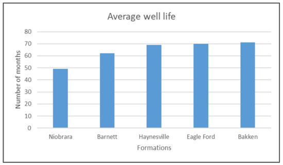
Figure 1.
Average well life for each formation.
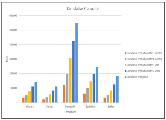
Figure 2.
Average cumulative production volumes after entire well’s life, two years, one year, six months, and three months for all wells from each formation. BOE: barrel of oil equivalent.
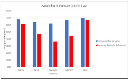
Figure 3.
Average drop in production from the maximum flow rate reached and from average flow rate for the first month within one year.
4. Production History Matching Using the Entire Production History
At the beginning of the study, production history matching was done between the entire actual production data with the DCA models. The objective of this step was to find the DCA model that best fit the production data and produced the most accurate ultimate recovery value. The iterative least-squares fitting method was performed on the production data with the SEPD and the Arps hyperbolic decline equations to find the optimum (fitted) values of the decline parameters for each model. For the SEPD model, the parameters were initial flow rate (qi), an exponent parameter (n), and a characteristic time parameter (τ), and for the Arps hyperbolic decline model, the parameters were initial flow rate (qi), a hyperbolic exponent (b), and the nominal 1/month decline rate (Di).
Table 3 represents the error analysis results from production history, matching between the entire production histories of the subject wells and the Arps hyperbolic decline model. Figure 4 shows an example of the matching with a well from one of the formations. The outcome of this production history matching is the decline parameters values for each well (qi, b, and Di) assuming them to be constant through the entire production period. Table 4 represents the error analysis results from production history matching between the entire production histories and the SEPD model. Figure 5 shows an example of the matching with a well from one of the formations. The outcome of this production history matching is the decline parameter values for each well (qi, n, and τ), assuming them to be constant through the entire production period. These resulting decline parameters were then used to calculate EUR for each well and compared with the actual EUR values measured using the cumulative production at the economic limit.
Table 3.
Error analysis results for production history matching using entire production history with the Arps hyperbolic decline model.
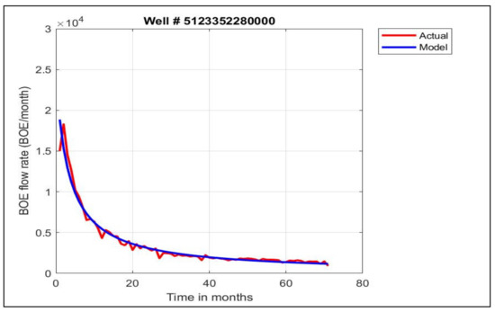
Figure 4.
Example of production history matching of entire production history data with the Arps hyperbolic decline model for a well in the Niobrara formation.
Table 4.
Error analysis results for production history matching using entire production history with the stretched exponential production decline (SEPD) model.
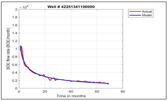
Figure 5.
Example of production history matching of entire production history data with the SEPD model for a well in the Barnett formation.
5. Production History Matching Using Limited Production History
Hindcasting is performed by matching a portion of the known production history and comparing the remaining portion of known production history to the forecast. Overall, the main objective for production history matching is to forecast production with high accuracy given only a short early production period. Therefore, production history matching was done using different early production periods (three months, six months, one year, and two years) and then compared to find the shortest production period needed to achieve reliable forecasts of EUR. Table 5 and Table 6 summarize the results from production history matching between different early production periods and Arps hyperbolic decline and SEPD models, respectively. Figure 6 and Figure 7 present examples of the outcomes of production history matching using early production data with Arps hyperbolic decline and SEPD models, respectively.
Table 5.
Results from production history matching on all wells from each formation using different production data periods with the Arps hyperbolic decline model.
Table 6.
Results from production history matching on all wells from each formation using different production data periods with the SEPD model.
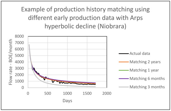
Figure 6.
Example of production history matching using different production history data with the Arps hyperbolic decline model for a well in the Niobrara formation.
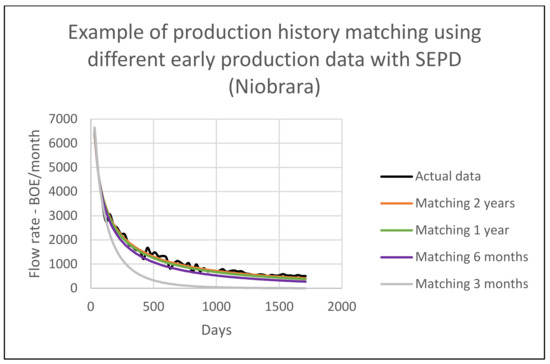
Figure 7.
Example of production history matching using different production history data with the SEPD model for a well in the Niobrara formation.
6. Assigning the Most Accurate Value for the Initial Flow Rate Parameter
Assigning an accurate value of initial flow rate (qi) is crucial to the success of production history matching as qi is always a main parameter in every DCA model. Initial flow rate could be assumed as the average production rate for the first month, first two months, first three months, or other values. Additionally, qi could be assumed as the maximum flow rate reached. The maximum flow rate was reached within the first three months of production in almost all the wells as shown in Figure 8. Production history matching using the entire production data was done on all the 1216 wells in this study while varying the value of qi to observe the change in accuracy of the fitted models with different qi values. Four different cases were investigated: (1) assuming qi was equal to the maximum flow rate reached, (2) assuming qi was equal to the average flow rate for the first month, (3) assuming qi was equal to the average flow rate for the first two month, and (4) assuming qi was equal to the average flow rate for the first three months.
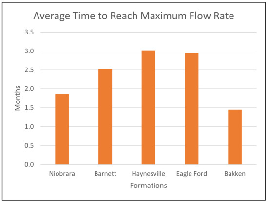
Figure 8.
Average time to reach maximum flow rate for all wells from each formation.
Figure 9 shows the different average values of qi for each formation between the four cases. Figure 10 compares the error in estimating EUR using the SEPD model between the four cases for each formation. Table 7 summarizes the mean absolute percentage error (MAPE) (%) of the four different cases for each formation.
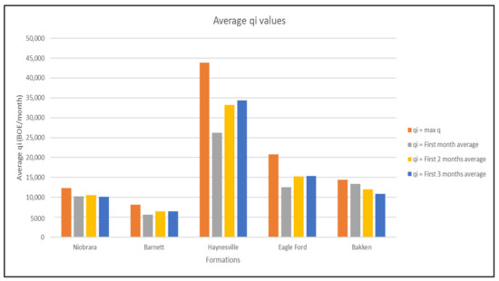
Figure 9.
Average of the four different values of initial flow rate definitions (qi) in BOE per month for all wells in each formation.
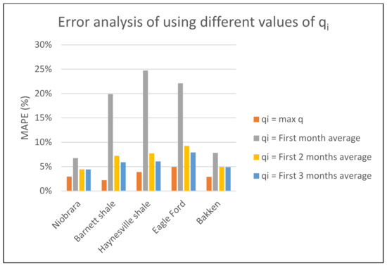
Figure 10.
Average MAPE of using four different values of initial flow rate definitions (qi) for all wells in each formation in calculating estimated ultimate recovery (EUR) using the SEPD model.
Table 7.
MAPE (%) of using different initial flow rate values in production history matching using the SEPD model.
7. Average Values of Decline Parameters
After performing production history matching for all the wells in the five formations using the entire production history for each well, average values of decline parameters were obtained for each formation. In this section, a comparison is presented between using the established average values of the decline parameters against production history matching using the different tested periods of production data. Table 8 summarizes the average values of decline parameters of the SEPD and Arps hyperbolic decline models for each formation. The accuracy in terms of correlation coefficient between actual and forecasted production by using the universal average decline parameters are summarized in Table 9.
Table 8.
Average decline parameters for all wells in each formation for the SEPD and Arps hyperbolic decline models.
Table 9.
Using average decline parameters error analysis in terms of correlation coefficient for all wells in each formation for the SEPD and Arps hyperbolic decline models.
8. Conclusions
In this study, production data analyses performed on 1216 multi-stage hydraulically fractured horizontal wells from five shale formations (Niobrara, Barnett, Haynesville, Eagle Ford, and Bakken) that were recently abandoned. Furthermore, production history matching with two DCA models was performed using least-square fitting on all the wells from this study. Following are the main highlights of this study.
Using two years of production data to match showed a mean absolute percentage error (MAPE) of less than 10% in EUR estimations across all wells from all five formations. The DCA model that provided the best fit varied between formations. For the Niobrara, Barnett, Eagle Ford, and Bakken formations, the Arps hyperbolic decline model showed higher accuracy of matching and forecasting production using limited early production data. While for the Haynesville formation, the SEPD model showed a higher accuracy in forecasting production using only a limited early production data. Across all wells in this study, four different initial flow rate values were investigated. In all 1216 wells from the five formations, assigning the initial flow rate as the maximum flow rate in the SEPD model resulted in the best estimates of EUR in production history matching. The maximum mean absolute percentage error (MAPE) when using the initial flow rate as the maximum flow rate was less than 5% in the production history matching performed in this study. Using other initial flow rate definitions increased the error greatly in all wells in the five formations. For the five studied reservoirs, the maximum flow rate was reached within the first three months of production for most of the wells. The main outcomes of the production history matching for all the wells using their entire production history were the DCA average parameters n and τ for the SEPD model and b and Di for the Arps hyperbolic decline model—for each formation. The accuracy of using average decline parameters of the Arps hyperbolic decline model provided a correlation coefficient between 0.77 and 0.85 for all the formations. For the SEPD model, a 0.60 to 0.83 correlation coefficient resulted when using the average decline parameters for all the formations.
Funding
This research received no external funding.
Institutional Review Board Statement
Not applicable.
Informed Consent Statement
Not applicable.
Data Availability Statement
Not applicable.
Acknowledgments
The author is grateful to the College of Petroleum Engineering and Geoscience, King Fahd University of Petroleum and Minerals. For its support in publishing this work.
Conflicts of Interest
The author declares no conflict of interest.
Nomenclature
| b | Hyperbolic exponent, dimensionless |
| BDF | Boundary dominated flow |
| Di | Nominal decline rate, 1/month |
| DCA | Decline curve analysis |
| EUR | Estimated ultimate recovery, BOE |
| n | Exponent parameter, dimensionless |
| qi | Initial flow rate, BOE/month |
| r | Pearson correlation coefficient, dimensionless |
| SEPD | Stretched exponential production decline |
| MAPE | Mean absolute percentage error, % |
| NRMSE | Normalized root mean square error, % |
| τ | Characteristic time parameter (Transition time), days |
References
- Rwechungura, R.W.; Dadashpour, M.; Kleppe, J. Advanced History Matching Techniques Reviewed. In Proceedings of the SPE Middle East Oil & Gas Show and Conference, Manama, Bahrain, 25–28 September 2011. [Google Scholar] [CrossRef]
- Arps, J.J. Analysis of Decline Curves. In Transactions of the AIME; Part II, SPE-945288-G; Society of Petroleum Engineers: Richardson, TX, USA, 1945; Volume 160, pp. 228–247. [Google Scholar] [CrossRef]
- Fetkovich, M.J.; Fetkovich, E.J.; Fetkovich, M.D. Useful Concepts for Decline Curve Forecasting, Reserve Estimation, and Analysis. SPE Res. Eng. 1996, 11, 13–22. [Google Scholar] [CrossRef]
- Lee, W.J.; Sidle, R.E. Gas Reserves Estimation in Resource Plays. In Proceedings of the SPE Unconventional Gas Conference, Pittsburgh, PA, USA, 23–25 February 2010. SPE-130102-MS. [Google Scholar] [CrossRef]
- Valko, P.P. Assigning value to stimulation in the Barnett Shale: A simultaneous analysis of 7000 plus production hystories and well completion records. In Proceedings of the SPE Hydraulic Fracturing Technology Conference, The Woodlands, TX, USA, 19–21 January 2009. [Google Scholar] [CrossRef]
- Kanfar, M.; Wattenbarger, R. Comparison of Empirical Decline Curve Methods for Shale Wells. In Proceedings of the SPE Canadian Unconventional Resources Conference, Calgary, AB, Canada, 30 October–1 November 2012. SPE-162648-MS. [Google Scholar] [CrossRef]
- Valko, P.P.; Lee, W.J. A Better Way to Forecast Production from Unconventional Gas Wells. In Proceedings of the SPE Annual Technical Conference and Exhibition, Florence, Italy, 19–22 September 2010. [Google Scholar] [CrossRef]
- Ilk, D.; Rushing, J.A.; Perego, A.D.; Blasingame, T.A. Exponential vs. Hyperbolic Decline in Tight Gas Sands: Understanding the Origin and Implications for Reserve Estimates Using Arps’ Decline Curves. In Proceedings of the SPE Annual Technical Conference and Exhibition, Denver, CO, USA, 21–24 September 2008. SPE-116731-MS. [Google Scholar] [CrossRef]
- Duong, A.N. Rate-Decline Analysis for Fracture-Dominated Shale Reservoirs. SPE Res. Eval. Eng. 2011, 14, 377–387. [Google Scholar] [CrossRef]
- Clark, A.J.; Lake, L.W.; Patzek, T.W. Production Forecasting with Logistic Growth Model. In Proceedings of the SPE Annual Technical Conference and Exhibition, Denver, CO, USA, 30 October–2 November 2011. SPE-144790-MS. [Google Scholar] [CrossRef]
- Zhang, H.; Cocco, M.; Rietz, D.; Cagle, A.; Lee, J. An Empirical Extended Exponential Decline Curve for Shale Reservoirs. In Proceedings of the SPE Annual Technical Conference and Exhibition, Houston, TX, USA, 28–30 September 2015. [Google Scholar] [CrossRef]
- De Holanda, R.W.; Gildin, E.; Valco, P.P. Combining Physics, Statistics, and Heuristics in the Decline-Curve Analysis of Large Data Sets in Unconventional Reservoirs. SPE Res. Eval. Eng. 2018, 21, 683–702. [Google Scholar] [CrossRef]
- Miao, Y.; Lee, J.; Zhao, C.; Lin, W.; Li, H.; Chang, Y.; Zhou, Y.; Li, X. A New Rate-Decline Analysis of Shale Gas Reservoirs: Coupling the Self-Diffusion and Surface Diffusion Characteristics. J. Pet. Sci. Eng. 2018, 163, 166–176. [Google Scholar] [CrossRef]
- Mahmoud, O.; Ibrahim, M.; Pieprzica, C.; Larsen, S. EUR Prediction for Unconventional Reservoirs: State of the Art and Field Case. In Proceedings of the SPE Trinidad and Tobago Section Energy Resources Conference, Port of Spain, Trinidad and Tobago, Spain, 25–26 June 2018. [Google Scholar] [CrossRef]
- Wilson, A. Comparison of Empirical and Analytical Methods for Production Forecasting. J. Pet. Technol. 2015, 67, 133–136. [Google Scholar] [CrossRef]
- Enverus Website. Available online: https://Enverus.com (accessed on 1 February 2019).


Publisher’s Note: MDPI stays neutral with regard to jurisdictional claims in published maps and institutional affiliations. |
© 2021 by the author. Licensee MDPI, Basel, Switzerland. This article is an open access article distributed under the terms and conditions of the Creative Commons Attribution (CC BY) license (http://creativecommons.org/licenses/by/4.0/).