1. Introduction
Alzheimer’s disease (AD) is by far the most common type of dementia, generally seen in elderly people. For the majority of cases, AD symptoms begin to appear during the mid-60s, although the early-onset may occur in ages as early as the 30s. It is estimated that around 106 million people will be diagnosed in the world by 2050 due to the increase in the aging population [
1].
During the progression of AD, the brain structure changes due to the deposition of amyloid-
(A
) plaques and hyperphosphorylated tau. The initial damage starts at the hippocampus [
2], which handles episodic and spatial memory as well as working as a relay between the brain and the rest of the body, so the damage disrupts these pathways. The symptoms of AD are the result of these A
plaques and intracellular neurofibrillary tangles [
3,
4]. This decreases the brain metabolism of both glucose and oxygen, leading to progressive memory loss and inability to move in the late stages [
5]. These changes start to form years before the initial clinical symptoms of AD are seen. Mild cognitive impairment (MCI) causes cognitive changes to the person that is noticeable by the family members and friends, but the person may still carry out daily activities. It’s been estimated that 15% to 20% of people over the age of 65 have MCI [
6]. Not every case progresses into dementia; in some individuals, MCI remains stable throughout their lives [
7]. The stages of AD progress can be seen as low-intensity brain cell activity in medical images. Positron emission tomography (PET) is an imaging technique that uses radiotracers to measure the metabolic processes, and magnetic resonance imaging (MRI) is another imaging technique that uses strong magnetic fields, magnetic field gradients, and radio waves. Resting-state functional magnetic resonance imaging (fMRI) is also considered a promising biomarker; however, in more severe cases, may cause problems due to the fMRI being very sensitive to head motion, mitigating its usefulness [
8]. PET imaging provides substantially sensitive assays, easily detecting a very low concentration of molecules of interest labeled through positron emitters, and MRI suffers from very low molar sensitivity for different metabolites and probes. This, coupled with the absolute quantification of substrate concentration being more challenging with MRI, PET imaging is generally chosen for AD imaging [
9]. Different types of nuclear tracers are developed for various purposes to highlight different parts of the body; some of the radiotracers that are used to detect A
plaques in the brain are florbetapir 18F, flutemetamol F18, PiB, and florbetaben 18F [
10]. Unfortunately, at the time of writing this paper, there is no definite cure for AD, and most of the treatments aim at alleviating the disease-related symptoms.
Beginning from the early 1970s, multiple computer-aided diagnostics (CAD) systems were proposed. Their early versions were usually based on manually extracted feature vectors [
11]. Later, these vectors were trained in a supervised method with a machine-learning model such as a support vector machine (SVM) [
12] to classify the input vector. It was soon realized that there were many shortcomings to such systems [
13]. Researchers turned towards data mining approaches in the 1980 and 1990s to develop more robust and flexible systems to overcome these limitations.
With the improvements to imaging methodologies, machine learning methodologies have been proposed to detect AD. These studies generally have multiple steps: feature extraction, feature selection, dimensionality reduction, and feature-based classification algorithm selection [
14]. The main issue with such works has been the reproducibility of these approaches [
15]. As an example, during the feature selection process, features that are related to AD are chosen from various modalities which may include cortical thickness, brain glucose metabolism, subcortical volumes, and cerebral A
accumulation in regions of interest (ROI), such as the hippocampus [
16]. Recent works make use of multi modalities of MRI, PET, and fMRI images, and use various preprocessing techniques such as segmentation [
17] to improve the accuracy of their proposed models [
18].
Recent developments in deep learning technology have led to a massive surge of constantly-improving models, especially in the computer vision area, mainly due to the improvements brought by convolutional neural networks (CNNs). These models learn to extract meaningful features from inputs and produce highly accurate results. The replacement of human experts with automated systems in the near future is being discussed due to the reduced cost and relatively similar performance [
19].
Anomaly detection is defined as the recognition of an unexpected pattern that is significantly different from the rest of the data. The majority of the challenges include a proper feature extraction method, imbalance in the data distribution, variance in anomalous cases, and environmental conditions. In the field of computer vision, anomaly detection is recently gaining more attention due to the advancements in the machine learning area. A key handicap with the public datasets is that most of these datasets have an imbalance among the classes they contain. The bias makes using such datasets difficult, especially in medical imaging, causing trained models to have less than desired performance [
20]. Furthermore, manual labeling of the medical imaging data is a costly and labor-intensive process, and considering the deep learning models thriving with large amounts of data, developed systems may end up with limited utility and poor generalization [
21]. In such scenarios, an unsupervised approach to data distribution modeling can be feasible, where the majority of the normal case data is used for training, and abnormal case data and the remainder of the normal case data are used to find outlier cases during the inference. For a variety of domains [
22,
23,
24], different approaches to anomaly detection [
25,
26,
27] have been proposed in the past. It is generally assumed that the anomalies differ in lower dimensions as well as in high-dimensional space, meaning the latent space mapping is a vital point in anomaly detection. Recent studies that include generative adversarial networks (GANs) [
28] in their models are highly effective in mapping the data distribution. GANs being efficient in mapping both high-dimensional and low-dimensional features with very little information loss has sparked a new interest in anomaly detection works [
29].
In medical imaging, GANs are generally used for AD diagnosis [
30], and data generation to be used in training the deep learning models [
31]. Anomaly detection can be used to differentiate normal brain images and the abnormal brain images is not very well researched.
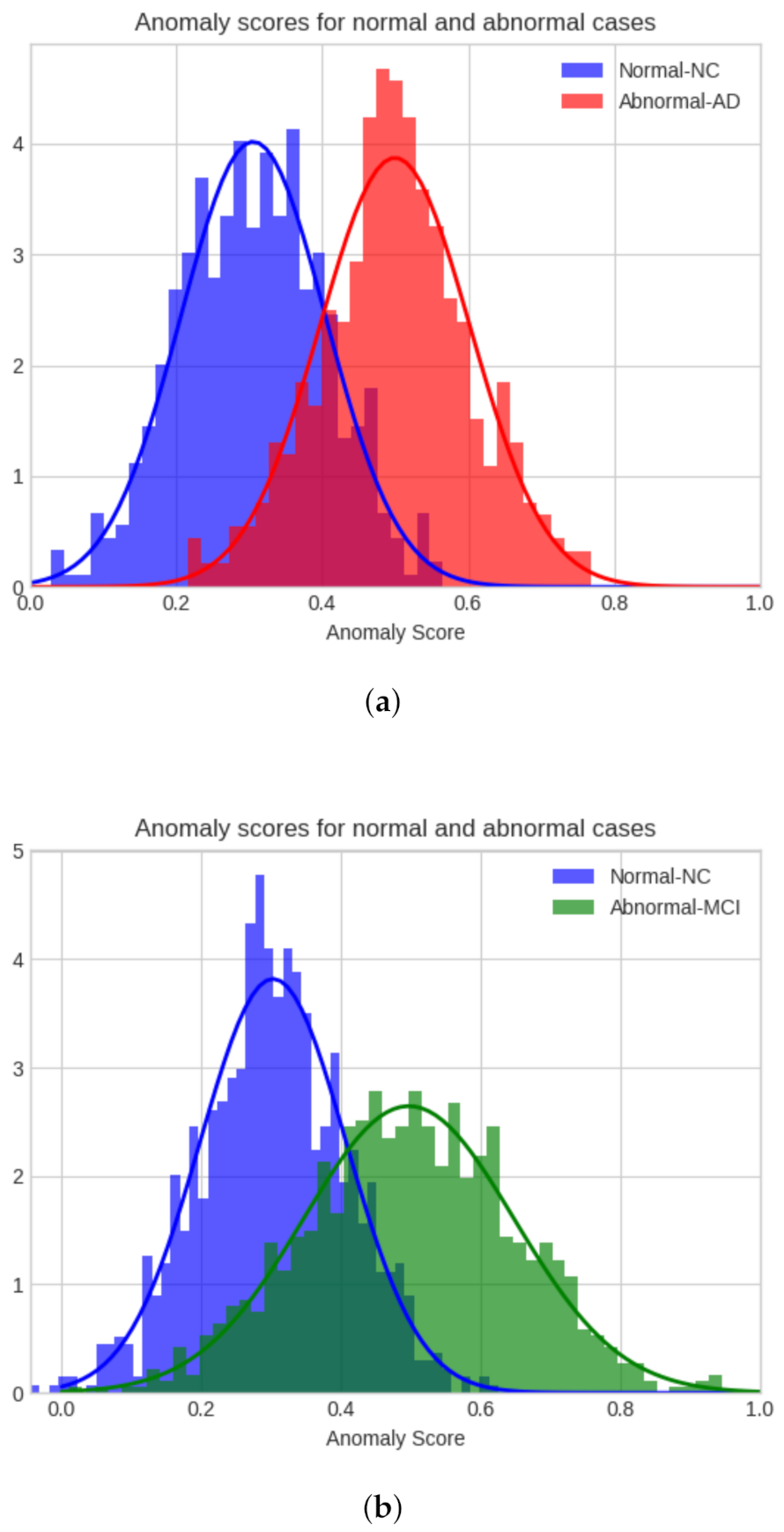
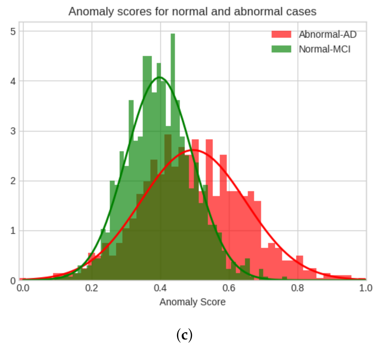
In this study, the analysis of Alzheimer’s disease as an anomaly using the proposed model is researched. In the Alzheimer’s Disease Neuroimaging Initiative (ADNI) dataset, there are three classes which are AD, MCI, and normal control (NC). The proposed model is trained using the unsupervised method. The anomaly analysis is performed on these classes in the following cases: AD-NC, MCI-NC, AD-MCI, the initial class is the anomaly class, and the latter class, the normal class. The area under the curve (AUC) is calculated for each of these comparisons to evaluate the performance of the model, as per previous work in the field [
32,
33], as well as Fréchet Inception Distance as a qualitative evaluation. Contributions of this paper are as follows:
Novelty—the Alzheimer’s disease anomaly analysis of PET images using a proposed unsupervised adversarially trained model with a unique feature extractor model. To the authors’ knowledge, there are no anomaly detection studies in Alzheimer’s disease cases using adversarial deep learning models.
Effectiveness—the proposed model quantitatively and qualitatively outperforms the state-of-the-art models.
2. Related Anomaly Detection Works
For better observation of the changes in the brain caused by AD, there has been a tremendous effort in the medical imaging field. Multiple machine learning applications have been proposed to classify different stages of AD using brain images [
34,
35,
36]. Different imaging techniques such as PET [
37,
38], structural magnetic resonance imaging (sMRI) [
39,
40], functional magnetic resonance imaging (fMRI) [
18,
41,
42] have been used in AD diagnosis. It has also been shown that multi-modal use may increase the performance compared to a single modal [
43]. For example, using the ADNI dataset, Lie et al. [
44] propose a multi-modality CNN model for binary classification of AD vs. NC with a classification score of 93.26%. Singh et al. [
45] achieved a remarkable 97.37% F1 score with their proposed method. Various implementations of GANs in medical imaging have also opened new possibilities from image segmentation [
46] to image translation [
47].
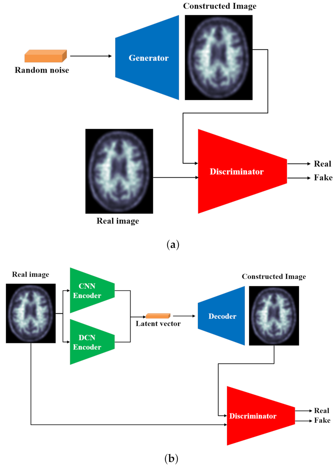
GANs are a type of generative machine learning framework that includes a generator that creates realistic images, usually from random noise, and a discriminator that identifies if the input image is real or fake. The generator is usually a decoder that learns the input data distribution from the latent vector, and the discriminator generally has a classic architecture that reads the input image and discriminates fake images from real images. The comparison between the novel GAN framework and the proposed model can be seen in
Figure 1.
Due to their potential uses, GANs have been examined in great depth [
48] and many approaches have been proposed to improve their stability [
49]. A well-known work, called Deep Convolutional GAN (DCGAN) [
50], removes fully-connected layers and makes use of convolutional layers and batch normalization [
51]. With the use of Wasserstein loss, the performance is improved even further [
52].
Recent attention on anomaly detection tends to be reconstruction-based. One study from Ravanbaksh et al. [
53] takes advantage of image-to-image translation [
54] to detect abnormality in crowded scenes. The approach uses two conditional-GANs; the first generator constructs an optical flow from input frames, and the second one generates frames from the generated flow. The main breakthrough comes from Schlegl et al.’s work [
23] where it is hypothesized that the end latent vector is a direct representation of the data distribution; however, mapping it is not a straightforward process. The first step is training a generator and a discriminator using only normal images, and afterward, remapping to the latent vector by freezing the weights based on the
z vector. The model shows the anomaly score during the inference by pinpointing an anomaly. Furthering this study, Zenati et al. [
32] (EGBAD) uses BiGAN [
55], examining joint training to map the data distribution end from the image and latent space, respectively. Akcay et al. [
29] propose the use of a conventional autoencoder (GANomaly) with the addition of another encoder the decoder to jointly train the model and the discriminator with the additional latent space loss. Furthering their work, Akcay et al. [
56] propose a U-Net-like [
57] autoencoder model (Skip-GANomaly) with skip-connections trained jointly with a discriminator.
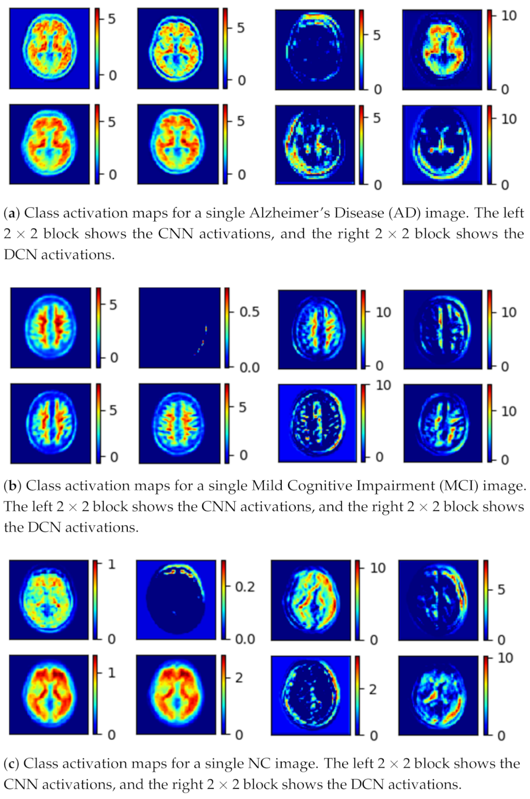
The human brain has a structure with many unique features that can be extracted by different CNN models. However, the majority of the works focus on creating a single complicated pipeline to extract these features. This study uses a parallel model that has been proven [
58] to extract more features than a single pipeline, which are reflected in its class activation maps during the inference. Furthermore, while the conventional GANs generate images from random input noise, the proposed model generates images from an input brain image, resulting in more realistic images. The findings of the experiment are explained and shown in the following sections.
3. Proposed Model
The proposed model uses an unsupervised adversarial training scheme. It has two major components:
The generator (G) learns the dataset distribution from the input image, encodes it into a latent vector, and reconstructs the image by upsampling. The uniqueness of the generator is that the encoder uses a parallel model that is comprised of a convolutional pipeline (CNN) and a dilated convolutional end network (DCN) that is 8 layers deep, each layer uses convolutional filters, a Rectified linear unit (ReLU) activation function, and a batch normalization operation. After two identical layers, a max-pooling operation is used for spatial dimension reduction and doubling the depth of the tensor. A latent vector of the input image is then generated.
The DCN is eight layers deep, each layer uses
convolutional filters with a dilation factor of 2, a ReLU (Rectified linear units) activation function, and a batch normalization operation. After 2 identical layers, a max-pooling operation is used for spatial dimension reduction and increasing the depth of the tensor. A latent vector of the input image is then generated. Concatenation of these features gives the optimal feature vector of the input image [
58]. The class activation map for the given input image is shown in
Figure 3.
The discriminator (D) predicts the class of the input (whether it is fake or not) based on learned features. The discriminator generally uses an encoder-type architecture.
The mathematical definition and the formulation of the problem are the following:
The dataset is split into a training set D that is comprised of N normal images where , and a testing set D̂ of A normal and abnormal images combined where denotes normal and abnormal class labels, respectively. The task is training the proposed model f on D and perform inference on A. Ideally, the training set should be larger than the training set, . Training helps to map the distribution of the dataset D in all vector spaces. This enables the network to learn both higher and lower-level features that are different from abnormal samples.
As shown in
Figure 2, the proposed model consists of a generator
G and a discriminator
D. The generator uses an autoencoder-type structure to generate an image
x̂ through extracted latent vector
z from the input image
x such that
where
and
. The input image
x is fed to both pipelines where the conventional CNN extracts local features and the DCN extracts global features. Concatenation of these features creates the latent vector
z. The convolutional network pipeline consists of eight convolutional layers, each layer is created using
convolutional filters, a ReLU activation, and a batch normalization operation. The DCN consists of 8 dilated convolutional layers with each layer being comprised of a
convolutional filters with a dilation factor of 2, a ReLU activation, and a batch normalization operation. At the end of each pipeline, extracted image features are concatenated to the create the latent vector to
z.
The decoder network consists of four upsampling layers and eight convolutional layers with convolutional filters on each layer, and a ReLU activation. Its task is to upsample the latent vector z back to its original input image dimension which is denoted as x̂.
Unsupervised training is performed with the majority of the normal class in the proposed GAN-based anomaly detection. In all three cases, the train-test split is the same. Eighty percent of the NC data is used to train the model, and the remaining 20% is used together with a similar number of AD images to detect the AD as the anomaly, or MCI as the anomaly with the NC, or the AD as the anomaly with the MCI dataset. The model is trained with only MCI data to distinguish AD, and MCI and AD data are considered abnormal data.


