Article

Health-Monitoring Methodology for High-Temperature Steam Pipes of Power Plants Using Real-Time Displacement Data

1
R&D Planning Office, KEPCO Research Institute, 105 Munji-ro, Yuseong-gu, Daejeon 34056, Korea
2
Department of Mechanical Engineering, Jeonbuk National University, 567 Baekje-daero, Deokjin-gu, Jeonju-si 54896, Korea
*
Author to whom correspondence should be addressed.
Appl. Sci. 2021, 11(5), 2256; https://doi.org/10.3390/app11052256
Submission received: 6 February 2021 / Revised: 24 February 2021 / Accepted: 26 February 2021 / Published: 4 March 2021
(This article belongs to the Special Issue Reliability of Materials and the Systems: Volume II)

Abstract

:
We developed a health-monitoring methodology for high-temperature steam pipes that estimated the life prediction of creep–fatigue interaction by directly measuring the displacement of hot parts. Three different methods (boiler code, design stress, and operating stress) were used to estimate the stress of the high-temperature pipe system. As a theoretical approach, the German boiler standard code calculates the stress according to the pipe shape, while design stress, which is also called allowable stress, was determined by a function of the operating temperature. The operating stress was immediately calculated using the surrogate model, with maximum displacement measured using the 3D displacement measurement system. To achieve the surrogate model, the stress was estimated by the pipe-stress analysis under the given displacements, and the surface-response model was developed to relate the stress and displacement. We showed that those methods are efficient methods to predict the stress and are applicable in health-monitoring methodology. Finally, the creep life and the low-cycle fatigue life were investigated using the Larson–Miller parameter equation, as well as the Smith, Hirschberg, and Manson equations. Our proposed monitoring system can be used to predict the fatigue and creep life of high-temperature steam pipes in real time, and we believe that the system can be applied to actual maintenance in thermal power plants.

1. Introduction

Life prediction of industrial facilities after many years of service is an important issue related to the stability, economy, and replacement of an entire facility. Since power plants require a huge cost when replacing typical parts or an entire facility, this problem is especially important in the field. The stable operation and reduction of the costs of life evaluation of facilities subjected to mechanical and thermal loads have been continually studied, and it is necessary to develop new approaches in assessing the residual life. Among the key components of power plants, steam pipes, which are designed to carry pressurized steam and are exposed to high temperatures, are in an extreme environment during operation. Thus, periodic maintenance through life prediction of steam pipes is essential.
It is known that steam pipes are mainly damaged by creep and fatigue, which are the main damage mechanisms that can be confirmed by metallurgical examinations. Creep and fatigue are already well-established failure modes for such components at room temperature. However, the failure mode becomes more complicated when the components are exposed to high temperatures during operation. Creep–fatigue interaction is the complex mode produced by cyclic and persistent mechanical loads, and it is depicted as the accumulated rate of damage under complex loadings. Fatigue failure is a mechanism involving crack propagation, while creep is manifested by the mobility of voids on the interior grain boundaries. Therefore, in the circumstances of high temperature with cyclic loadings, creep–fatigue interaction, which shows creep cavitation and surface-fatigue damage, may be found within the material and should be considered when evaluating life prediction.
From a microscopic viewpoint, crack behaviors have been determined according to operating environments such as cyclic loadings or creep. For low cyclic loadings, the transgranular fracture has been frequently observed because cracks propagate through the grains after they are initiated in a material. At low and intermediate stress, the creep failures occur due to the initiation and growth of creep cavitation or a void along the grain boundaries, which is called intergranular fracture, and the grain boundaries are weakened by the formation of the creep cavitation or a void. The intergranular creep failure follows the process of nucleation, growth, interlinkage of cavities, crack propagation, and fractures. During the creep–fatigue interaction, the creep failure within the material and fatigue damage on the surface are both present. The crack path in the creep–fatigue interactions consists of both the transgranular and intergranular fractures. Once the crack is initiated by the creep–fatigue cycling, it propagates through the interior grains, and the crack path evolves from a mixed mode to intergranular as the hold time is increased. Therefore, the life prediction of creep–fatigue interaction is quite complicated due to the mixed mode of transgranular and intergranular fractures.
The life-prediction methods in the creep–fatigue interaction can be categorized into four main models: the linear-damage summation model [1,2,3,4], the ductility-exhaustion model [5,6,7], strain-range partitioning [8], and the hysteresis-energy-related damage parameter [9,10,11,12,13]. The first approach to estimate the total life in creep–fatigue interaction is the linear-damage summation method, which is an empirical model. Spera [1] proposed the linear-damage summation method based on works by Miner [3] and Roinson [4]. It is assumed that the fracture occurs when the addition of time-dependent (creep) and time-independent (fatigue) damages reaches unity. The linear-summation rule leads to conservative estimates of life, and has been widely used because it is the procedure advocated by the ASME Boiler and Pressure Vessel Code [14]. In the ductility-exhaustion model, the fatigue and creep damaging processes compete to cause failures [6]. It is assumed that, during the creep–fatigue interaction, damage evolution gradually processes with the ductility exhaustion of the materials and fails completely once the accumulated strain reaches a critical ductility. The strain-range partitioning method [8] isolates the overall creep–fatigue damage into the summation of the damage fraction determined by a separated strain range. According to the strain-range partitioning method, the strain range during a single cycle can be separated into subcycles, and the median cyclic fatigue life can be calculated by linear damage accumulation with partitioned strain ranges. Ostergren [9] proposed the strain energy damage function model, which assumes that only tensile inelastic strain energy can induce the crack opening and propagation. In fact, only the deformation occurring in the tensile portion of the cycle with the crack open can contribute to the damage by propagating the crack. According to the strain energy damage function model, the fatigue life is related to the strain energy and material constants utilized in the Coffin–Manson equation. In this paper, we adopted the linear-summation rule for life prediction subjected to creep–fatigue interaction because of its conservative and robust nature among the life-prediction methods.
Recently, theoretical and experimental studies have been conducted to predict fatigue [15,16,17,18,19,20] and creep [21,22,23,24] life for parts exposed to high temperatures and cyclic loads. Various evaluation methods (i.e., strain energy density, stress-based method, strain range method, linear-damage summation method, and ductility-exhaustion model) were used to evaluate the creep and fatigue life according to the loading conditions and the shape of the specimen. However, the previous studies were to prove the validity of the life-evaluation method or to predict the lifespan of the current state, and no studies were conducted to evaluate lifespan in real time. To the best of our knowledge, although deformation or displacement measurement in real time for health monitoring [25,26,27] have been conducted, the measured displacement-based life prediction in real time has not been studied and developed yet. There are several limitations to monitoring the life prediction in real time and utilizing it for maintenance. To evaluate life in real time, it is necessary to construct a complex model and perform analysis through various input conditions, which increases the time required for creep–fatigue life evaluation. Recently, surrogate models [28,29,30,31,32] have been used to reduce the time required for the analysis of complex models without sacrificing accuracy and detail. Surrogate modeling is widely used in engineering design loops and can be applied to various engineering problems. Surrogate models are also computationally cheaper and can approximate complex models. In this study, an efficient method for life prediction for a main steam pipe is proposed using the three-dimensional displacement measurement system (3DDMS) and surrogate models developed by a stress-based approach. The aim of the proposed study was to develop a health-monitoring methodology for high-temperature piping to maintain the system and for periodic maintenance through life prediction of the steam pipe. The 3DDMS was utilized to measure the displacements of the main steam pipe, and a series of pipe-stress analyses were performed to calculate the stress level within a measured displacement. Based on the stress and function of the measured displacements, we developed a surrogate model, correlating stress and displacement and life prediction under the creep–fatigue interaction. Our work implemented the stress analysis and life assessment of the piping system for the Manjung power plant in Malaysia, and it shows that the proposed method is quite a reasonable and reliable system for the stress and life assessment of high-temperature steam pipes.

2. Stress-Calculation Methodologies for High-Temperature Steam Pipes

Three methods were used to calculate the stress of the high-temperature pipe system in this study: The German boiler standard Technical Rules for Steam Boilers (TRD) code method uses the geometric information of pipes, the yield strength-based method estimates the design stress, and the 3DDMS method obtains the operating stress at maximum displacement through the proposed surrogate model.

2.1. TRD-Code-Based Method

The main steam pipe (MSP) of the Manjung power plant has straight, bent, and T-piece components, and it measures 445 mm in outer diameter with a thickness of 41.5 mm and a tolerance of 12.5%. The piping stiffness and section modulus are based on the nominal wall thickness, which decreases by tolerance percentage. The formula for calculating the stress according to the pipe shape in the TRD code is shown in Table 1.
To verify the calculations for the completed components, the wall thickness, straight pipe, and cross-section values should be calculated as shown in Table 1. The s v , s e , and s o are the wall thicknesses of many bodies; c 1 and c 2 are allowance under tolerances or corrosion; and v N indicates the weld joint factor. Solving for the reference Tresca, i.e., the stress used for the remaining life calculations based on uniaxial test results, the stresses of the external diameter can be calculated. When the pressure is 19.4 MPa, the welding coefficient is 1, and when s v is 36.3125, the calculated stress is 99.471 MPa. According to the TRD code, two stresses must be calculated for the elbows: the average stress inside the bend and the average stress outside of the bend. The four stresses (two stresses each for the given inside/outside diameters) are calculated according to Table 1. Depending on the given values (either the outside diameter of the cylindrical shell ( d a ) or the inside diameter of the cylindrical shell ( d i )), the average stress of both outside the bend ( σ i ¯ ) and inside the bend ( σ a ¯ ) must be calculated. When the bending radius is 2250 mm and the curvature radius is 2757 mm, the internal stress is 110.23 MPa and the external stress is 110.14 MPa. For the stress calculation of T-pieces, it is necessary to distinguish among three types: extruded branch, forged branch, and branch with/without reinforcement. In the case of the Manjung power plant, the forged branch should be considered to calculate the stress for the T-piece piping components. Nevertheless, for all three types of T-pieces, the values e G and e A in Table 1 must be calculated. Drawings suitable for the planimeter are used to obtain the pressure loaded area ( A P ) and cross-sectional area ( A σ ) as functions of e G and e A , respectively. For the extruded branches, if the extension radii are not considered, the cross-sectional area A σ should be multiplied by a factor of 0.9. The average stress is then calculated by geometrical conditions. The stress of the T-piece pipe calculated using the equation in Table 1 is 103.9 MPa.

2.2. Design-Stress-Based Method (Allowable Stress)

It is well known that all components of a power plant are manufactured by considering the design pressure or stress. In this study, allowable stresses were used to increase the reliability of the life and risk evaluation results. P91 and X20CrMoV121 steels were simultaneously used for the main steam piping of large coal-fired power plants. Since the design stress is determined by the temperature at which the target material is used, the correlation equation of temperature can be obtained from the allowable stress curve for each temperature of P91 through a regression method. Without any information about stress in relation to the operating condition and geometric dimensions, allowable stress can be represented as a function of operating temperature [33]:
σ a l l o w = A 0 + A 1 T + A 2 T 2
where A 0 is −134.92, A 1 is 1.30388, and A 2 is −0.001618 for P91 steel. In actual operating conditions, the stress value is 91.2 MPa at the maximum operating temperature of 552   , and the stress value is 96.47 MPa at the average operating temperature of 542   .

2.3. DDMS-Data-Based Method

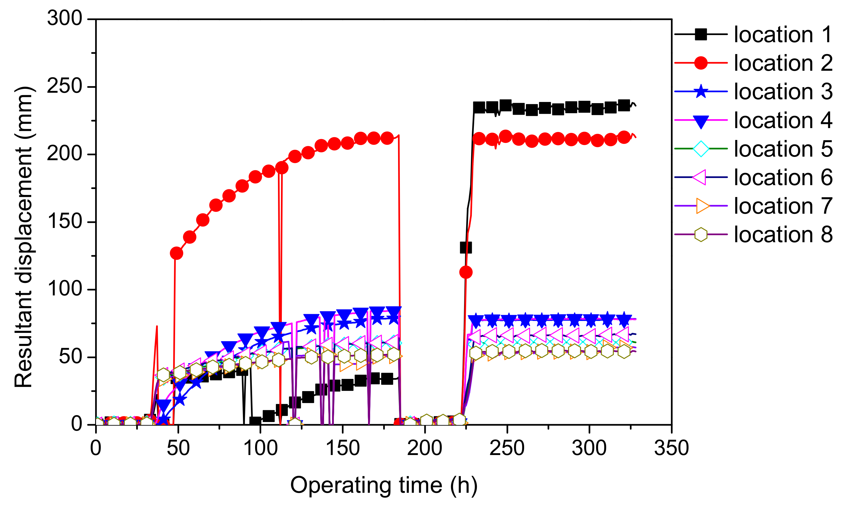
The power-plant boiler, which is the subject of this study, is equipped with a system that can measure the 3D displacement of pipes, as shown in Figure 1. The displacements of each location are measured by 3DDMS, as presented in Figure 2. The location of the vulnerable part where the actual maximum stress occurs is different from the location where the 3D displacement is measured. The maximum displacements were selected to calculate each location’s stress. The stress value according to the displacement at the location where 3DDMS was installed was calculated using CAESARII [34], a pipe-only analysis program, to derive the displacement–stress correlation equation. The verification of CAESARII was reported to be in good agreement with experimental results according to a previous study [35]. In this study, the code is used to evaluate the stress generated by the main steam pipe. The stress results based on the maximum displacement at each location are shown in Table 2.
On the other hand, the welding part of the H-joint of the main steam pipe does not have 3DDMS installed, but it is potentially a weak part where macrocracks were observed during regular inspections during the maintenance period [36]. In this study, the stress of the H-joint from the relative displacement at locations 7 and 8 presented in Figure 3a was evaluated by the pipe-stress analysis, in addition to the existing positions 1–8. Theoretically, stresses at the H-joint can be increased directly by unsynchronized movements at locations 7 and 8. We observed that the displacement differences in the x and z directions were relatively high; therefore, those differences were used to calculate the stress at the H-joint. The shape of the H-joint adjacent to locations 7 and 8 with 3DDMS installed and the response surface graph showing the stress relationship in the H-joint according to the changes of x and z are shown in Figure 3b. The response surface model for calculating the stress according to the displacement differences in the x- and y-axes is shown in Equation (2). The stress data, as well as the parameters related to Equation (2), are shown in Table 3 and Table 4, respectively.
σ = γ 1 + γ 2 Δ x + γ 3 Δ z + γ 4 Δ x Δ z + γ 5 Δ z 2
where σ indicates the stress at the H-joint, and Δ x and Δ z are the movement differences between locations 7 and 8 in the x- and z-directions, respectively. The maximum displacement and calculated stresses are shown in Table 2; it was observed that the stress at the H-joint was relatively large. Thus, regarding locations 1–8, it was necessary to investigate the creep and fatigue life of the H-joint.
Table 5 shows the stress values calculated through the three methods described in Section 2. Since it was necessary to evaluate the life based on the maximum stress value in order to monitor the service life considering the stability of the facility, the maximum value of the stress calculated by each method was selected. According to Table 5, the TRD method considered the shape and operating conditions that had the maximum stress value in the straight and the bent pipes. On the other hand, in the case of the H-joint pipe, the stress calculated by the response surface method based on the three-dimensional displacement value had a maximum value.

3. Life Evaluation for High-Temperature Steam Pipes

3.1. Creep Life Prediction

Many methodologies are based on time-temperature parameters that relate the stress and temperature to time-to-failure. One advantage of using time–temperature parameters is the possibility to create master curves, which allows easy interpolation and extrapolation of data. In this paper, the Larson–Miller parameter was used to calculate the creep life for the high-temperature piping systems. The Larson–Miller parameter (LMP) is the most universally used parameter today to assess creep damage. As shown below, creep damage is a function of temperature, stress, and time. Creep damage was calculated by curve fitting through the Larson–Miller parameter using the National Institute for Materials Science (NRIM) creep test data [37]. The NRIM test results for calculating creep and the LMP curve fitting equation and graph are shown in Figure 4. LMP is a function of temperature and design life, and it can be expressed as follows:
L M P = ( T + 273 ) ( C + log t r ) = B 0 + B 1 log σ + B 2 log σ 2
In the case of P91, the LMP is presented in Table 6. From the estimated LMP, the creep rupture time, which is also called the creep design life, is expressed as:
t r = 10 1000 L M P T + 273 C
Creep life, which is also called the creep life consumption rate ϕ c r e e p , is calculated as follows:
ϕ c r e e p = t o p t r
where t o p and t r indicate the operating hours and the creep rupture time, respectively. Finally, the maximum creep life among the three results with the 3DDMS, TRD, and allowable stress methods was selected and used to calculate the total life of the target component, i.e., the main steam piping.

3.2. Low-Cycle Fatigue Life Prediction

For high-temperature components, it is well-known that creep is the dominant damage mechanism, and low cycle fatigue (LCF) damage is relatively negligible for boiler components such as pipes and tubes. However, in this study, the LCF life was calculated to quantify the LCF damage rate and to check whether the 3DDMS data were used to calculate the LCF life. The LCF damage was calculated by conducting curve fitting through the LCF test data [38]. It was observed that the cyclic strain process of the P91 steels proceeded with a dominant participation of the elastic strain component. In the elastic range (below 450 MPa), the maximum stress can be directly converted to strain values, since the strain is proportional to stress according to Hook’s law. The fatigue life of the P91 material described by the Smith, Hirschberg, and Manson dependence [1,2,3,4] is expressed as:
Δ ε t = Δ ε e + Δ ε p = G / E N f v + M N f z
where G , E , and N f indicate the shear modulus, elastic modulus, and fatigue durability, respectively. In addition, v and z are the material constants. All parameters of the fatigue model are presented in Table 7. The fatigue durability can be determined from Equation (6) by using the Newton–Raphson method. The LCF life is determined as follows:
ϕ L C F = N o p N t
where N o p and N t indicate the number of start-ups and the number of cycles to failure, respectively.
In this study, the LCF life was calculated using two types of cycle-counting methods, which were number of cycle counting (NCC) and rainflow cycle counting (RCC). In the case of the NCC method, the maximum stress or strain during start-ups (i.e., cold) is used to calculate the fatigue life by only considering the number of starts N o p . In contrast, the RCC method determines the load cycles for closed hysteresis loops in a loading history, and all 3DDMS data are used as loading history for the count cycle. Among the two results by each method, the maximum LCF life is used to calculate the total life with maximum creep life. The total life consumption after the N o p of start-ups and an operating time t o p is determined by using a nonlinear accumulation damage rule [7] as follows:
ϕ T o t a l = ϕ C R E E P + ϕ L C F + e ϕ C R E E P ϕ L C F r
The hyper-parameter e and r that determine the nonlinear interaction effects are assumed to be fixed to certain values under conservative assumptions. As a result, appropriate e and r values should be used to evaluate the life under actual operating conditions. In this study, we assumed that e was 0.75 and r was 0.5 when considering the creep and fatigue interactions in high chromium alloy steel, which is a representative material of power-plant facilities [39,40,41].

3.3. Lifetime Prediction

To calculate the lifetime of plant facilities, basic data such as operating conditions and hours or number of cycles are essential. Because a lifetime is related to the dominant damage mechanism and damage model, various data are used to calculate the life consumption rate. In the case of the Manjung power plant, creep damage is more dominant than LCF because the operation has been running for a long time (i.e., 88,311 operating hours) and the number of cycles (i.e., 50 cold, 23 warm, 66 hot) is too small. The material subjected to a high-temperature greater than 0.4 to 0.5 of the melting temperature will slowly deform under loads that would not cause any plastic deformation at room temperature. Creep stresses at this temperature are expressed by a typical result of creep tests and extrapolation of data for the long-time creep phenomenon. The strain not only depends on the stress, but also depends on temperature and time.
The creep life consumption rate was evaluated by the stress-based life prediction methods such as TRD, allowable stress, and 3DDMS. In addition, the LCF life consumption rate was calculated by both methods (NCC and RCC). The creep and LCF life consumption rates were chosen to be the maximum value of each method. The total life consumption rate was estimated using Equation (8). The total life consumption rates of different locations are presented in Table 8. For the MSP with straight type, most of the maximum creep life consumption rate was estimated by the TRD method, based on the theoretical equation using geometric information. However, the creep life consumption rate calculated by the 3DDMS method had a maximum value at position 1. The 3DDMS method determined the stress according to the displacement because the displacement at location 1 was the largest compared to locations 7 and 8, which were constrained adjacent to the turbine.
For the LCF life prediction, both the rainflow cycle and the number of cycles showed a lower value of life consumption rate, which was compared with the creep life consumption rate. It was noted that the creep was a more dominant factor of life prediction than low cycle fatigue because the operating hours were relatively longer than the number of cycles. In the case of MSP with the H-joint type, the total life consumption rate where the creep life consumption rate was the dominant factor showed a relatively higher value. From the stress analysis, the maximum stress of MSP was observed at the curved edge of the H-joint, due to the role of stress concentration of the curved edge. Thus, the pipe system that was subjected to high temperatures was easily exposed to creep damage, and especially, creep damage accumulated more at the curved edge.

4. Development of the Health-Monitoring Program for the High-Temperature Steam Pipes

Facilities operating in harsh environments, such as power-plant boilers, evaluate the health of the facility, i.e., the service life in the future, through regular preventive maintenance. For the health monitoring of the main steam pipe, in this study, the quantification of the damage and the prediction of the remaining service life at the H-joint followed the procedure suggested by Rytter [42]. As mentioned in the introduction, in order to evaluate the life of the main steam pipe, the degree of damage due to creep and fatigue damage, known as the main damage mechanism, must be calculated. In particular, in the case of H-joints made of welds, the degree of damage was quantified as a life consumption rate as mentioned in Section 2 and Section 3 because it was more vulnerable due to cracks and residual stress. As a consequence, software was developed that could predict the remaining life by calculating the life consumption rate according to the displacement, and through this, a study was conducted to monitor the health of the main steam pipe.
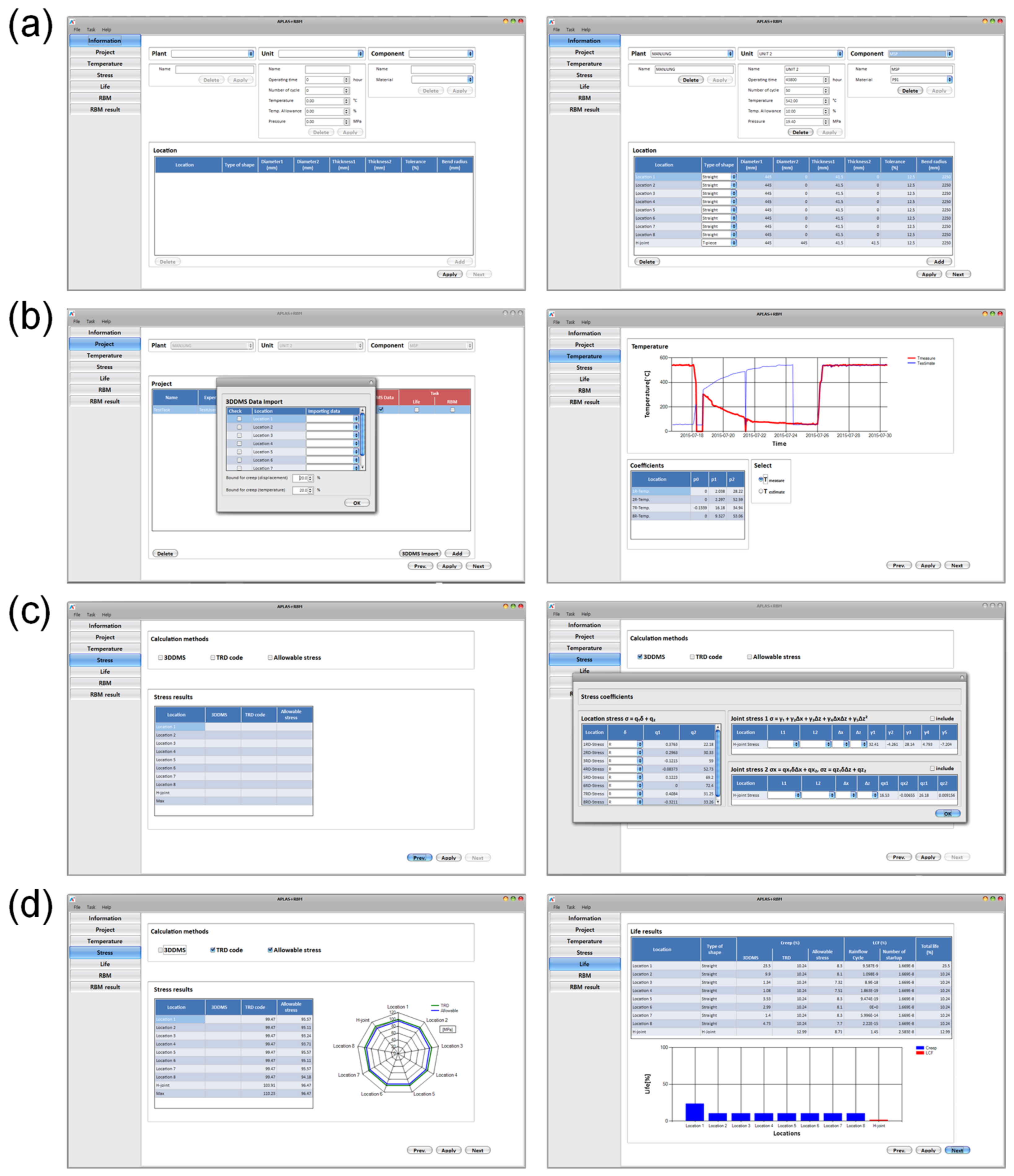
A program that calculates the lifetime has been developed using three methods of calculating stress for hot steam pipes, as shown in Figure 5. Temperature can be estimated by inputting basic information such as power plant, unit, operation information, and piping material, as shown in Figure 5a, and then importing 3D displacement data for each location, as shown in Figure 5b. As shown in Figure 5c,d, the stress is calculated by 3DDMS, TRD code, and allowable stress, and finally, the lifetime of each location is calculated using the creep and fatigue damage model. The creep panel shows the creep life through each stress method using Equations (3) and (4). The LCF panel shows the fatigue life through an iterated calculation using rainflow cycle counting.

5. Conclusions

In this study, we developed a health-monitoring methodology and software for the high-temperature steam pipes of operating power plants. The proposed monitoring software can evaluate fatigue and creep life for the actual power-plant system in real time. To evaluate stress in the high-temperature stream pipes, we adopted three different methods—boiler code, design stress, and operating stress. As a theoretical approach, stress according to the pipe shape (i.e., straight, bent, and T/Y piece) was estimated by the German boiler standard TRD code, and allowable stress (or design stress) was presented as a function of operating temperature. In addition, the operating stress was calculated by the pipe-stress analysis software called CAESARII under the measured displacements by 3DDMS and operating temperature as boundary conditions. When developing a new methodology under laboratory conditions, separate validation is required for field application, but in this study, data from a 3D displacement system, installed in an actual power plant boiler located in Manjung Malaysia, was used for methodology development. Based on the actual operating stress data, we proposed a response surface model to calculate the operating stress according to the measured displacement by 3DDMS in real time. Finally, the creep life and the low-cycle fatigue life were investigated by the Larson–Miller parameter equation and the Smith, Hirschberg, and Manson equations, respectively. Through this method, a health-monitoring methodology that can predict stress in real time was developed, and a stress-based life-evaluation-monitoring analysis software was completed.
The health-monitoring methodology proposed in this study provides real-time stress and theoretical stress evaluation equations for the high-temperature steam pipes of operating power plants, and based on this, creep and fatigue life evaluations are possible. With the surrogate model, stress and life can be quickly calculated using only displacement information, making it easy to analyze the health of power-plant piping systems online and offline. The proposed monitoring system has already been applied an operating power plant in the Manjung power plant, and we believe this is a practical and meaningful study in that our method is currently being used for power-plant maintenance.

Author Contributions

Conceptualization, W.C. and J.H.; methodology, W.C. and J.H.; software, W.C.; validation, W.C. and J.H.; visualization, W.C. and J.H.; data curation, W.C.; investigation, W.C. and J.H.; writing—original draft preparation, W.C. and J.H.; review and editing, W.C and J.H.; supervision, J.H.; All authors have read and agreed to the published version of the manuscript.

Funding

This research was supported by the “Research Base Construction Fund Support Program” funded by Jeonbuk National University in 2021, the KEPCO Research Institute (No. R08GH21), and the National Research Foundation of Korea (NRF) grant funded by the Korean government (MSIT) (No.2020R1F1A1060442).

Institutional Review Board Statement

Not applicable.

Informed Consent Statement

Not applicable.

Data Availability Statement

Not applicable.

Conflicts of Interest

The authors declare no conflict of interest.

References

  1. Spera, D.A. A Linear Creep Damage Theory for Thermal Fatigue of Materials. Ph.D. Thesis, University of Wisconsin-Madison, Madison, WI, USA, 1968. [Google Scholar]
  2. Taira, S. Lifetime of Structures Subjected to Varying Load and Temperature. In Creep in Structures. IUTAM Symposia (International Union of Theoretical and Applied Mechanics); Hoff, N.J., Ed.; Springer: Berlin/Heidelberg, Germany, 1962. [Google Scholar]
  3. Miner, M.A. Cumulative Damage in Fatigue. J. Appl. Mech. 1945, 12, A159–A164. [Google Scholar]
  4. Robinson, E.L. Effect of Temperature Variation on the Long-Time Rupture Strength of Steels. Trans. ASME 1952, 74, 777–780. [Google Scholar]
  5. Polhemus, J.F.; Spaeth, C.E.; Vogel, W.H. Ductility Exhaustion Model for Prediction of Thermal Fatigue and Creep Interaction. In Fatigue at Elevated Temperatures; Carden, A.E., McEvily, A.J., Wells, C.H., Eds.; ASTM International: West Conshohocken, PA, USA, 1973; pp. 625–636. [Google Scholar]
  6. Priest, R.H.; Ellison, E.G. A Combined Deformation Map-Ductility Exhaustion Approach to Creep-Fatigue Analysis. Mater. Sci. Eng. 1981, 49, 7–17. [Google Scholar] [CrossRef]
  7. Goswami, T. Low Cycle Fatigue Life Prediction—A New Model. Int. J. Fatigue 1997, 19, 109–115. [Google Scholar] [CrossRef]
  8. Manson, S.S.; Halford, G.R.; Hirschberg, M.H. Creep-Fatigue Analysis by Strain-Range Partitioning. In First Symposia on Design for Elevated Temperature Environment; ASME: San Francisco, CA, USA, 1971; pp. 12–28. [Google Scholar]
  9. Ostergren, W.J. A Damage Function and Associated Failure Equations for Predicting Hold Time and Frequency Effects in Elevated Temperature, Low Cycle Fatigue. J. Test. Eval. 1976, 4, 327–339. [Google Scholar]
  10. Halford, G.R. Energy Required for Fatigue. J. Mater. 1966, 1, 3–18. [Google Scholar]
  11. Chiou, Y.C.; Yip, M.C. An Energy-Based Damage Parameter for the Life Prediction of AISI 304 Stainless Steel Subjected to Mean Strain. J. Chin. Inst. Eng. 2006, 29, 507–517. [Google Scholar] [CrossRef]
  12. Fan, Z.; Chen, X.; Chen, L.; Jiang, J. Fatigue–Creep Behavior of 1.25Cr0.5Mo Steel at High Temperature and its Life Prediction. Int. J. Fatigue 2007, 29, 1174–1183. [Google Scholar] [CrossRef]
  13. Lee, K.-O.; Hong, S.-G.; Lee, S.-B. A New Energy-Based Fatigue Damage Parameter in Life Prediction of High-Temperature Structural Materials. Mater. Sci. Eng. A Struct. 2008, 496, 471–477. [Google Scholar] [CrossRef]
  14. ASME. Standard Heat Treatments for Fabrication Processes: ASME Code for Pressure Piping, B31 ASME B31.1-2017; ASME: New York, NY, USA, 2017. [Google Scholar]
  15. Wang, Q.; Chen, J.; Chen, X.; Gao, Z.; Li, Y. Fatigue Life Prediction of Steam Generator Tubes by Tube Specimens with Circular Holes. Metals 2019, 9, 322. [Google Scholar] [CrossRef] [Green Version]
  16. Nilsson, K.-F.; Dolci, F.; Seldis, T.; Ripplinger, S.; Grah, A.; Simonovski, I. Assessment of thermal fatigue life for 316L and P91 pipe components at elevated temperatures. Eng. Fract. Mech. 2016, 168, 73–91. [Google Scholar] [CrossRef]
  17. He, X.; Chen, J.; Tian, W.; Li, Y.; Jin, W. Low Cycle Fatigue Behavior of Steam Generator Tubes under Axial Loading. Materials 2018, 11, 1944. [Google Scholar] [CrossRef] [PubMed] [Green Version]
  18. Arora, P.; Gupta, S.K.; Bhasin, V.; Singh, R.K.; Sivaprasad, S.; Tarafder, S. Testing and assessment of fatigue life prediction models for Indian PHWRs piping material under multi-axial load cycling. Int. J. Fatigue 2016, 85, 98–113. [Google Scholar] [CrossRef]
  19. Branco, R.; Costa, J.D.; Berto, F.; Antunes, F.V. Fatigue life assessment of notched round bars under multiaxial loading based on the total strain energy density approach. Theor. Appl. Fract. Mech. 2018, 97, 340–348. [Google Scholar] [CrossRef] [Green Version]
  20. Bertini, L.; Frendo, F.; Marulo, G. Fatigue life assessment of welded joints by two local stress approaches: The notch stress approach and the peak stress method. Int. J. Fatigue 2018, 110, 246–253. [Google Scholar] [CrossRef]
  21. Salifu, S.; Desai, D.; Kok, S. Numerical simulation and creep-life prediction of X20 steam piping. Mater. Today Proc. 2021, 38, 893–898. [Google Scholar] [CrossRef]
  22. Jing, H.; Su, D.; Xu, L.; Zhao, L.; Han, Y.; Sun, R. Finite element simulation of creep-fatigue crack growth behavior for P91 steel at 625 °C considering creep-fatigue interaction. Int. J. Fatigue 2017, 98, 41–52. [Google Scholar] [CrossRef]
  23. Xu, Q.; Yang, X.; Lu, Z. On the development of creep damage constitutive equations: A modified hyperbolic sine law for minimum creep strain rate and stress and creep fracture criteria based on cavity area fraction along grain boundaries. Mater. High Temp. 2017, 34, 323–332. [Google Scholar] [CrossRef] [Green Version]
  24. Salifu, S.; Desai, D.; Kok, S. Prediction and Comparison of Creep Behavior of X20 Steam Plant Piping Network with Different Phenomenological Creep Models. J. Mater. Eng. Perform. 2020, 29, 7382–7395. [Google Scholar] [CrossRef]
  25. Ghaffar, M.H.A.; Husin, S.; Baek, J.E. Application of displacement monitoring system on high temperature steam pipe. IOP Conf. Ser. Mater. Sci. Eng. 2017, 257, 012026. [Google Scholar] [CrossRef] [Green Version]
  26. Hong, H.; Cai, Z.; Wang, W.; Liu., Y. An online monitoring method for creep-fatigue life consumption with real-time damage accumulation. Int. J. Damage Mech. 2021. [Google Scholar] [CrossRef]
  27. Zhang, H.; Jia, J.; Wang, N.; Hu, X.; Tu, S.-T.; Zhou, S.; Wang, Z. Development of On-Line Monitoring Systems for High Temperature Components in Power Plants. Sensors 2013, 13, 15504–15512. [Google Scholar] [CrossRef] [Green Version]
  28. Hussain, M.F.; Barton, R.R.; Joshi, S.B. Metamodeling: Radial basis functions versus polynomials. Eur. J. Oper. Res. 2002, 138, 142–154. [Google Scholar] [CrossRef]
  29. Kourakos, G.; Mantoglou, A. Pumping optimization of coastal aquifers based on evolutionary algorithms and surrogate modular neural network models. Adv. Water Resour. 2009, 32, 507–521. [Google Scholar] [CrossRef]
  30. Kennedy, M.C.; O’Hagan, A. Bayesian calibration of computer models. J. R. Stat. Soc. Ser. B 2001, 63, 425–464. [Google Scholar] [CrossRef]
  31. Yoon, H.; Jun, S.-C.; Hyun, Y.; Bae, G.-O.; Lee, K.-K. A comparative study of artificial neural networks and support vector machines for predicting groundwater levels in a coastal aquifer. J. Hydrol. 2011, 396, 128–138. [Google Scholar] [CrossRef]
  32. Laloy, E.; Rogiers, B.; Vrugt, J.A.; Mallants, D.; Jacques, D. Efficient posterior exploration of a high-dimensional groundwater model from two-stage Markov chain Monte Carlo simulation and polynomial chaos expansion. Water Resour. Res. 2013, 49, 2664–2682. [Google Scholar] [CrossRef] [Green Version]
  33. Becht, C. Power Piping: The Complete Guide to ASME B31.1; ASME Press: New York, NY, USA, 2013. [Google Scholar]
  34. CAESAR II Design Manuals; ASME Standards, B 31.3, BS 7159; ASME Press: New York, NY, USA, 2019.
  35. Lu, H.; Wu, X.; Huang, K. Study on the Effect of Reciprocating Pump Pipeline System Vibration on Oil Transportation Stations. Energies 2018, 11, 132. [Google Scholar] [CrossRef] [Green Version]
  36. Chu, Q.; Zhang, M.; Li, J.; Chen, Y.; Luo, H.; Wang, Q. Failure Analysis of a Steam Pipe Weld Used in Power Generation Plant. Eng. Fail. Anal. 2014, 44, 363–370. [Google Scholar] [CrossRef]
  37. Sawada, K.; Kimura, K.; Abe, F.; Taniuchi, Y.; Sekido, K.; Nojima, T.; Ohba, T.; Kushima, H.; Miyazaki, H.; Hongo, H.; et al. Catalog of NIMS Creep Data Sheets. Sci. Technol. Adv. Mater. 2019, 20, 1131–1149. [Google Scholar] [CrossRef] [PubMed] [Green Version]
  38. Junak, G. Low-cycle fatigue of P91 and P92 Steels Used in the Power Engineering Industry. Arch. Mater. Sci. Eng. 2011, 48, 19–24. [Google Scholar]
  39. Choi, W.; Yoon, H.; Youn, B.D. Operation-Adaptive Damage Assessment of Steam Turbines Using a Nonlinear Creep-Fatigue Interaction Model. IEEE Access 2020, 8, 126776–126783. [Google Scholar] [CrossRef]
  40. Rusin, A.M. Technical Risk Involved in Long-Term Operation of Steam Turbines. Reliab. Eng. Syst. Saf. 2007, 92, 1242–1249. [Google Scholar] [CrossRef]
  41. Pohja, R.; Holmström, S.; Nilsson, K-F.; Payten, W.; Lee, H.-Y.; Aktaa, J. Creep-Fatigue Interaction Rules for P91: MATTER—Deliverable D4.5; European Commission EC: Rome, Italy, 2014; p. 64. [Google Scholar]
  42. Rytter, A. Vibration Based Inspection of Civil Engineering Structures. Ph.D. Thesis, University of Aalborg, Aalborg, Denmark, 1993. [Google Scholar]
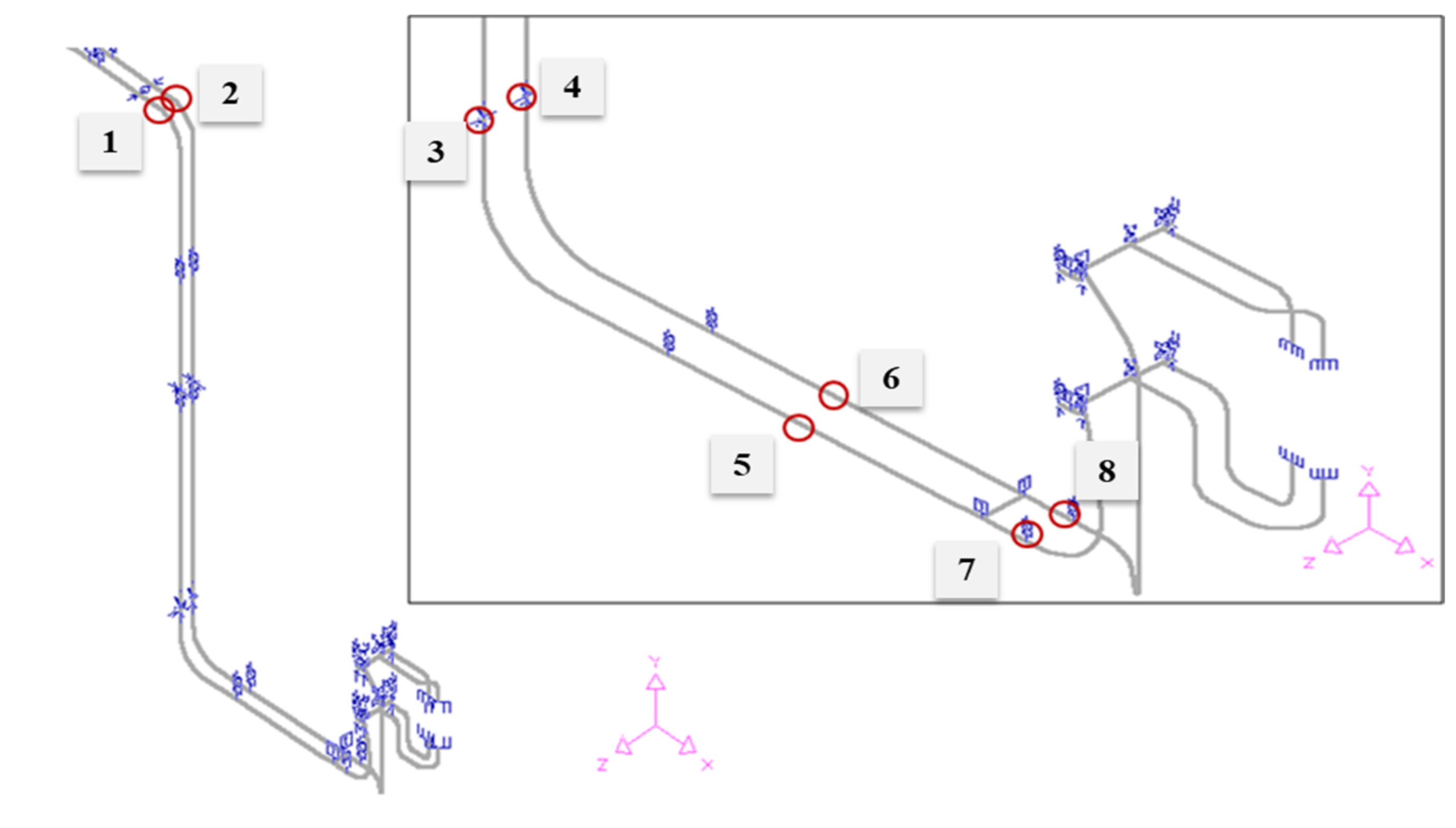
Figure 1. Modeling and 3D displacement measurement positions in the main steam pipe using CAESARII.
Applsci 11 02256 g001
Figure 2. The measured magnitude of displacements with respect to operating time at 3DDMS locations.
Applsci 11 02256 g002
Figure 3. Relationship between the displacement and stress at the H-joint: (a) the geometric model of the vicinity of the H-joint, and (b) response surface model for the H-joint.
Applsci 11 02256 g003
Figure 4. NRIM test results for creep life prediction: (a) Larson–Miller parameter, and (b) cumulative failure probability curve of P91 [37].
Applsci 11 02256 g004
Figure 5. Display of life-assessment software for piping systems: (a) basic information, (b) 3DDMS importing and temperature calculation, (c) stress calculation, and (d) life prediction.
Applsci 11 02256 g005
Table 1. Stress-calculation formula based on the TRD code.
GeometryDominant Formula
Straight σ = p 2 d a 2 s v v N s v
s v = s e c 1 c 2 , s v = s o v N
Bent σ i ¯ = p d a s v i s v a 2 s v i v N 2 R 0.5 d a + 1.5 s v i 0.5 s v a 2 R d a + s v i + p 2
σ a ¯ = p d a s v i s v a 2 s v a v N 2 R + 0.5 d a + 0.5 s v i 1.5 s v a 2 R + d a s v a + p 2
r = s v 1 2 d a 2 s v 2 + R s v 2 + 1 4 d a 2 s v 2 + R s v 2 2 d a 2 s v d a 2 s v 1 R s v 2
T/Y piece σ ¯ = p A p A σ + 1 2
A p = d i 2 e G + d A a 2 + d A i 2 e A + s v
A σ = s v e G + s A 0 e A + s v s A 0
e G = d i + s v s v , e A = 1.25 d A i + s A 0 s A 0
Table 2. Stress results estimated by CAESARII with 3DDMS data.
LocationMax. Magnitude of Displacement (mm)Von-Mises Stress (MPa)
1238.042112.35
2215.2194.76
379.04649.39
484.6545.64
561.9276.96
667.4672.40
761.4458.84
854.9813.69
H-jointDifference in displacement between
locations 7 and 8 (mm)
113.76
Δ x = 7.65 Δ z = 6.6
Table 3. Parameters of the stress-displacement relationship at the H-joint.
CoefficientsGoodness of Fit
γ 1 γ 2 γ 3 γ 4 γ 5 SSER-squareRMSE
32.41−4.26128.144.793−7.2042.3890.9990.7728
Table 4. Estimated stress of the H-joint with respect to the relative displacement.
Δ x Δ z Von-Mises Stress (MPa)
1.00.028.149
2.01.054.41
3.02.075.84
4.02.081.17
4.03.092.46
6.04.0111.23
7.656.6113.76
Table 5. Results of the stress calculation evaluated by three different methods.
LocationTypes3DDMS
(MPa)
TRD
(MPa)
Allowable
(MPa)
Maximum
Stress (MPa)
1Straight112.3599.4795.57112.35
294.7695.1199.47
349.3993.2499.47
445.6493.7199.47
576.9695.5799.47
672.4095.1199.47
758.8495.5799.47
813.6994.1899.47
H-jointT-piece113.76103.9196.47113.76
Table 6. Larson–Miller parameters of P91.
C B 0 B 1 B 2
28011.83413.67−4.51161
Table 7. Parameters of fatigue models for P91 steel.
G / E v M z
0.009−0.11.205−0.78
Table 8. Results of life consumption rate with different locations of the main steam pipe by considering the total operating hours.
LocationCreep Life Consumption Rate (%)LCF Life Consumption Rate (%)Total Life
Consumption
Rate (%)
3DDMSTRDAllowableRainflow CycleNumber of Cycles
123.510.248.33.34 × 10−95.82 × 10−823.5
29.98.13.82 × 10−105.82 × 10−810.24
31.397.323.18 × 10−185.82 × 10−810.24
41.057.516.49 × 10−205.82 × 10−810.24
53.538.33.09 × 10−195.82 × 10−810.24
62.998.105.82 × 10−810.24
71.48.32.09 × 10−145.82 × 10−810.24
80.177.77.74 × 10−165.82 × 10−810.24
H-joint36.6212.998.710.15.82 × 10−836.62
Publisher’s Note: MDPI stays neutral with regard to jurisdictional claims in published maps and institutional affiliations.