
Investigation of Deformation Inhomogeneity and Low-Cycle Fatigue of a Polycrystalline Material


Abstract
:1. Introduction
2. Material Model and Crystal Plasticity Model
2.1. Material
2.2. RVE Polycrystalline Material Model
2.3. Constitutive Model of Crystal Plasticity
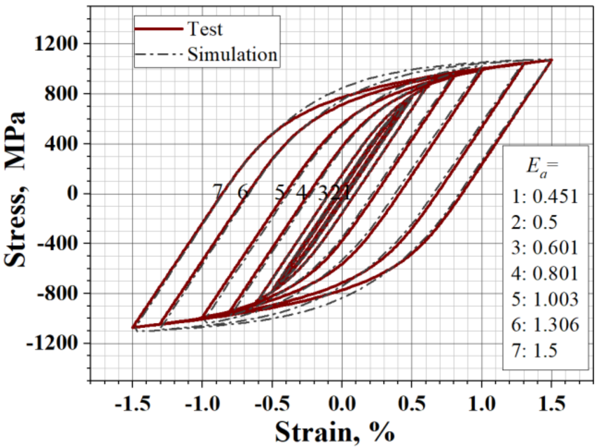
2.4. Parameter Calibration of Constitutive Model
3. Measurements of Deformation Inhomogeneity and Predictions of Fatigue–Life Curve
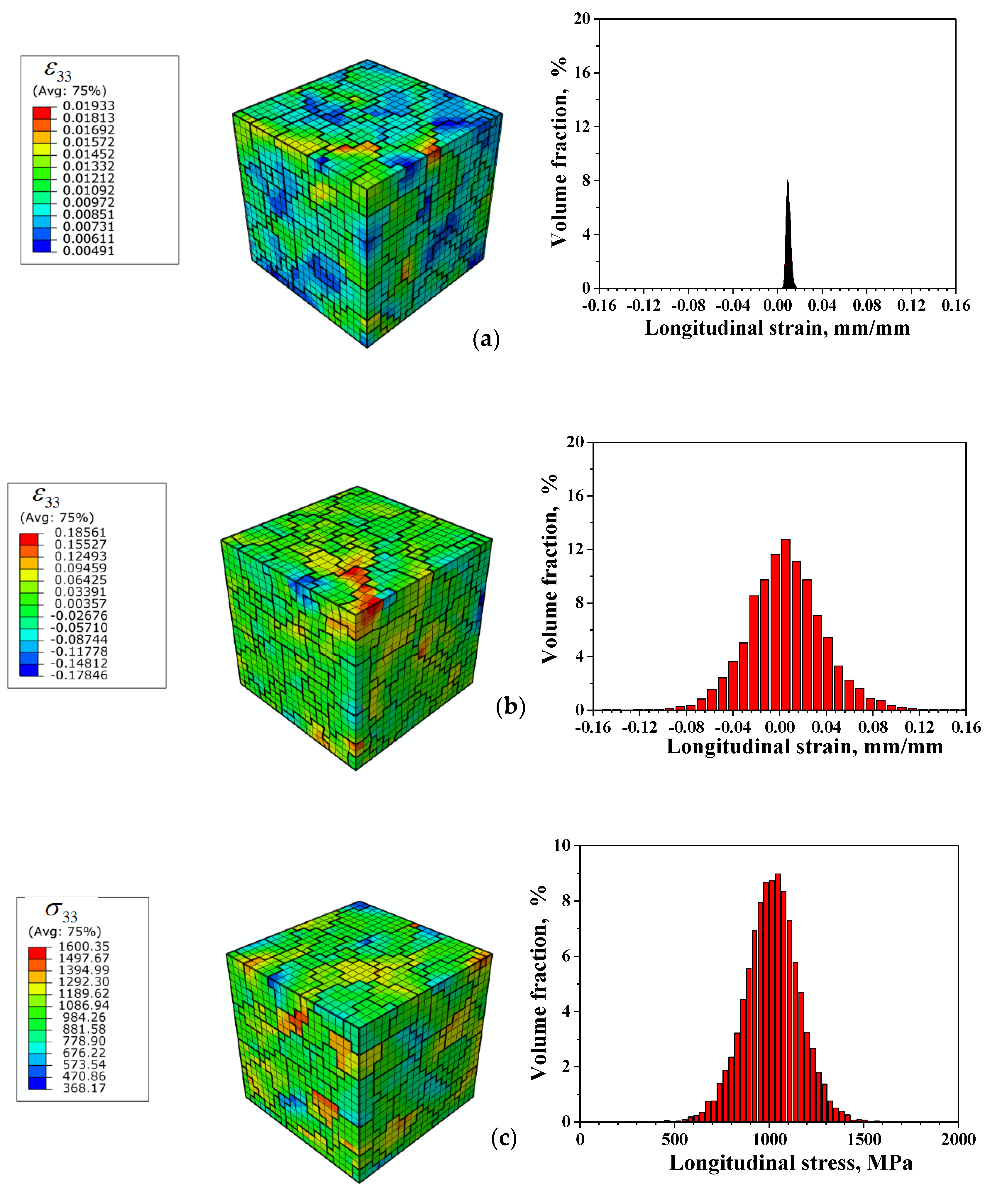
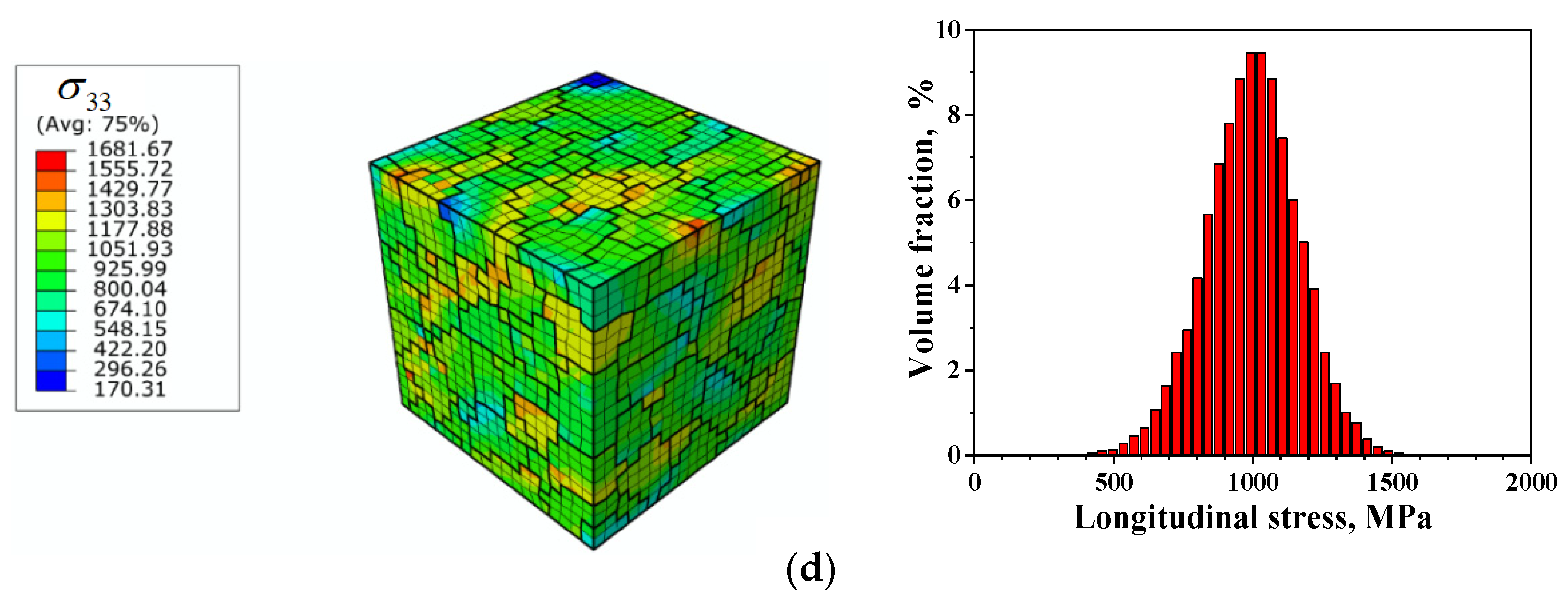
3.1. Distribution and Inhomodeneity of Strain and Stress in RVE
3.2. Different Measurement of Statistics of Strain Inhomogeneity
3.3. Fatigue Indicator Parameters (FIPs), Life Prediction and Verification
3.3.1. Inhomogeneity Measurement of Distribution of Different Strain Components
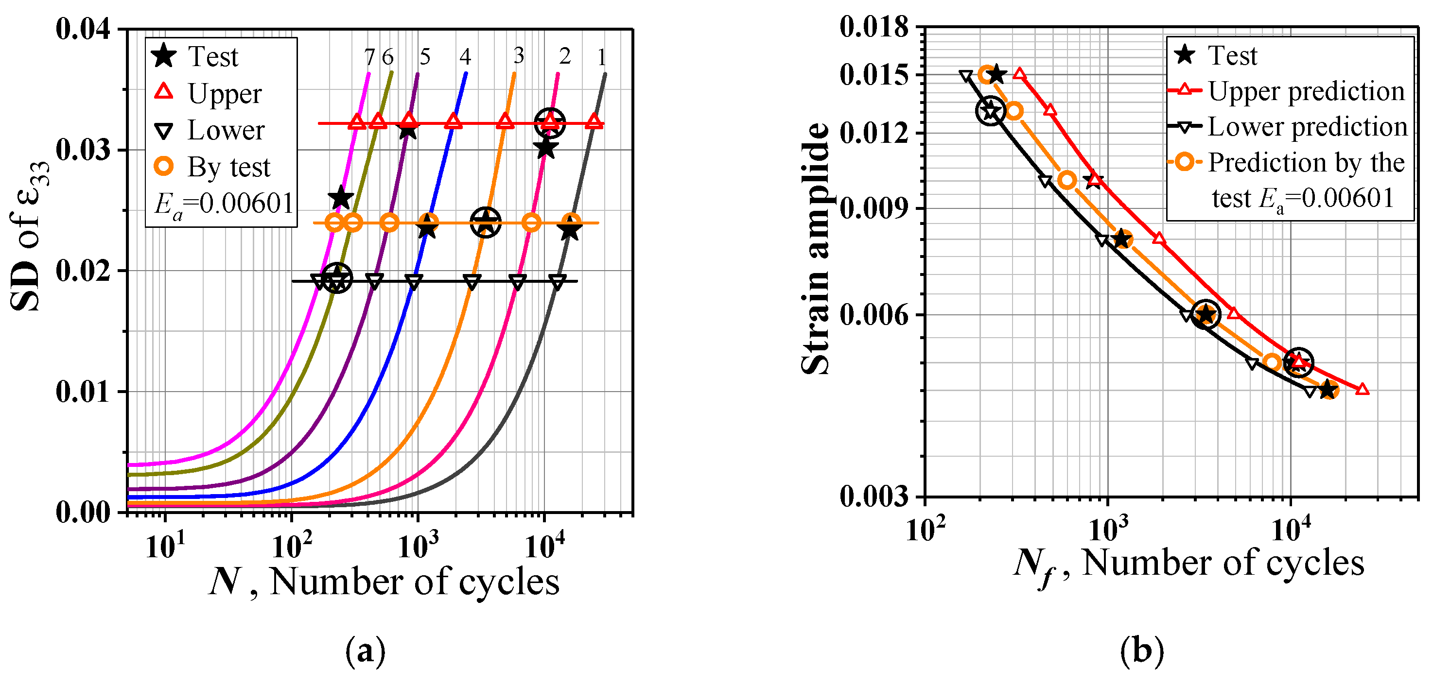
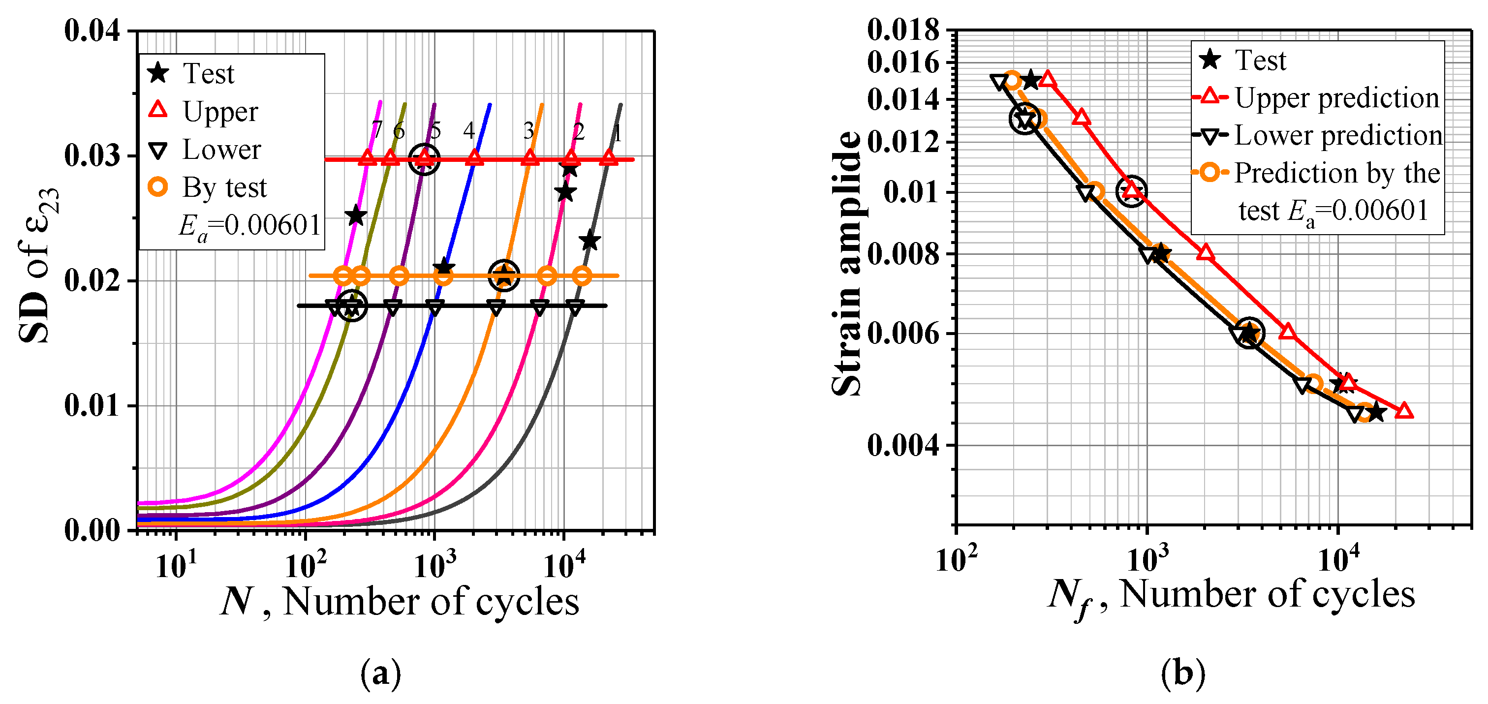
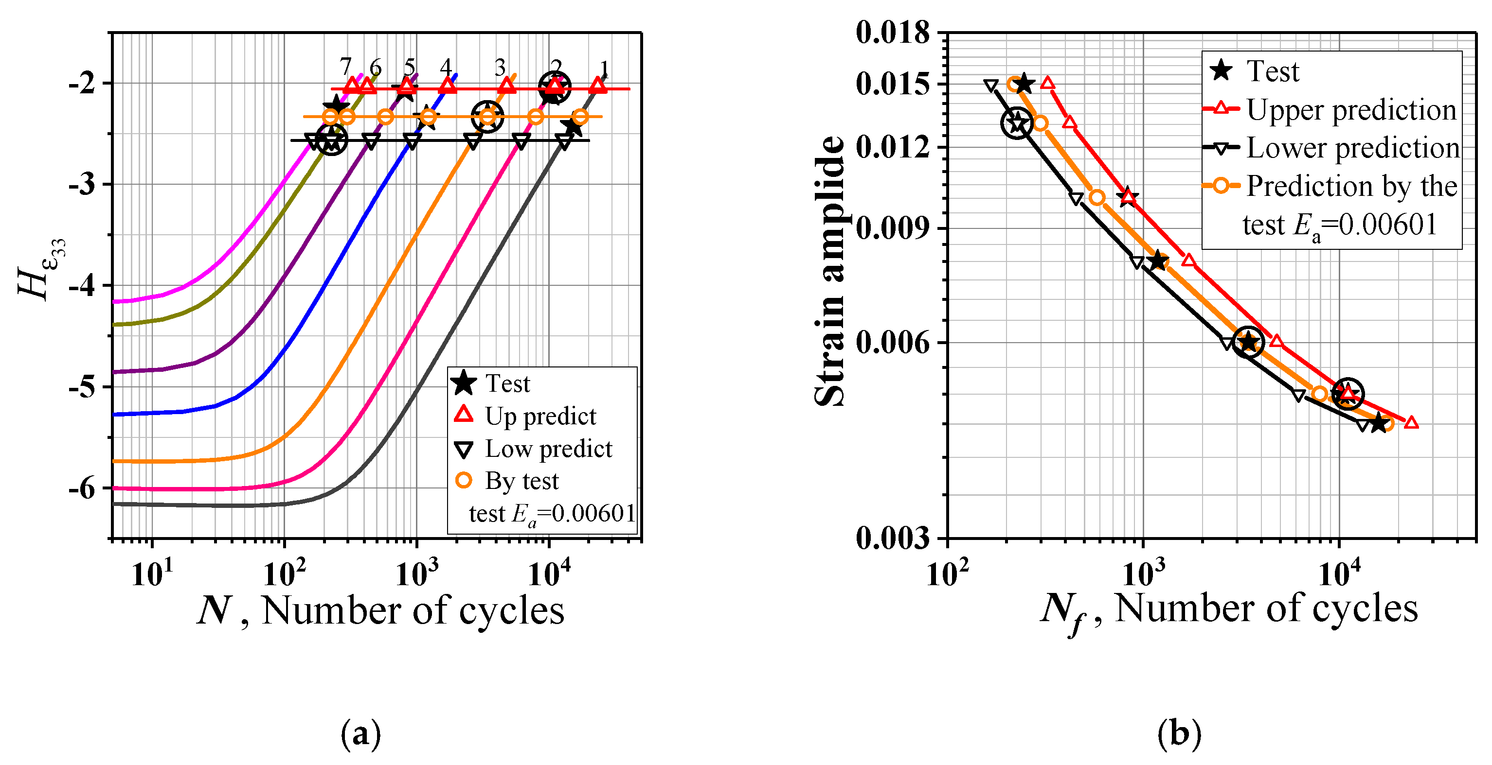
3.3.2. The Deformation Inhomogeneity Growing and Fatigue Failure Occurrence Predicting
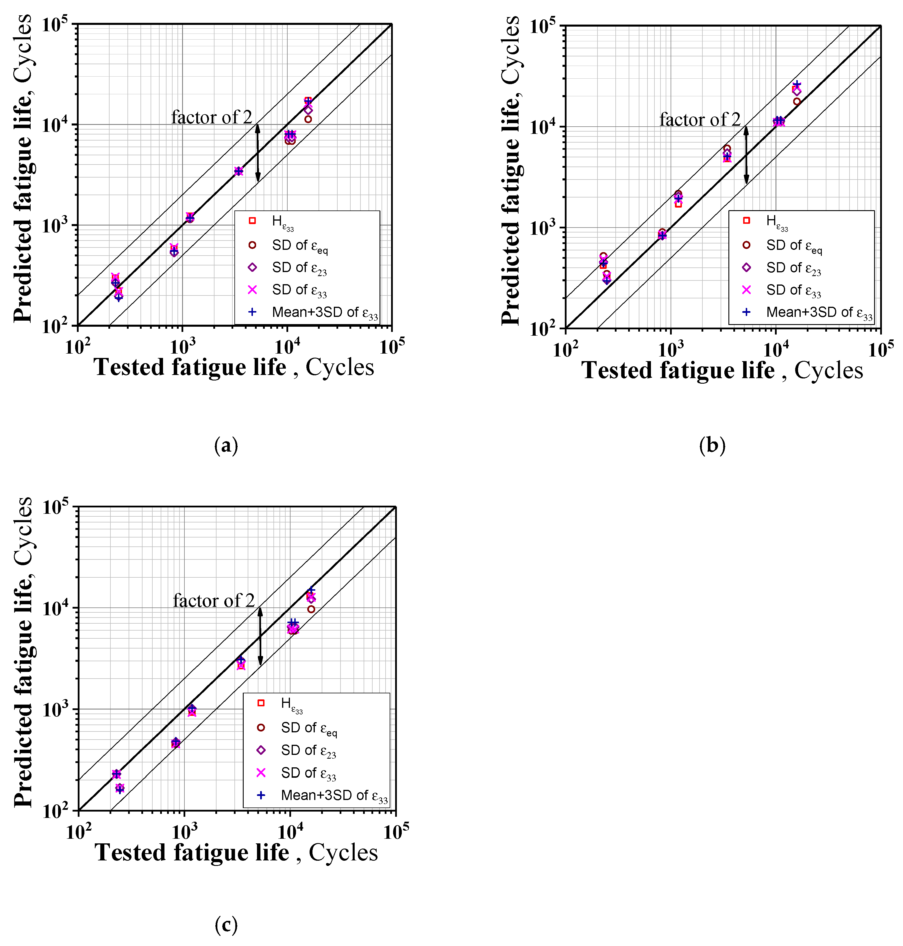
3.3.3. Validation
4. Discussion and Conclusions
- (1)
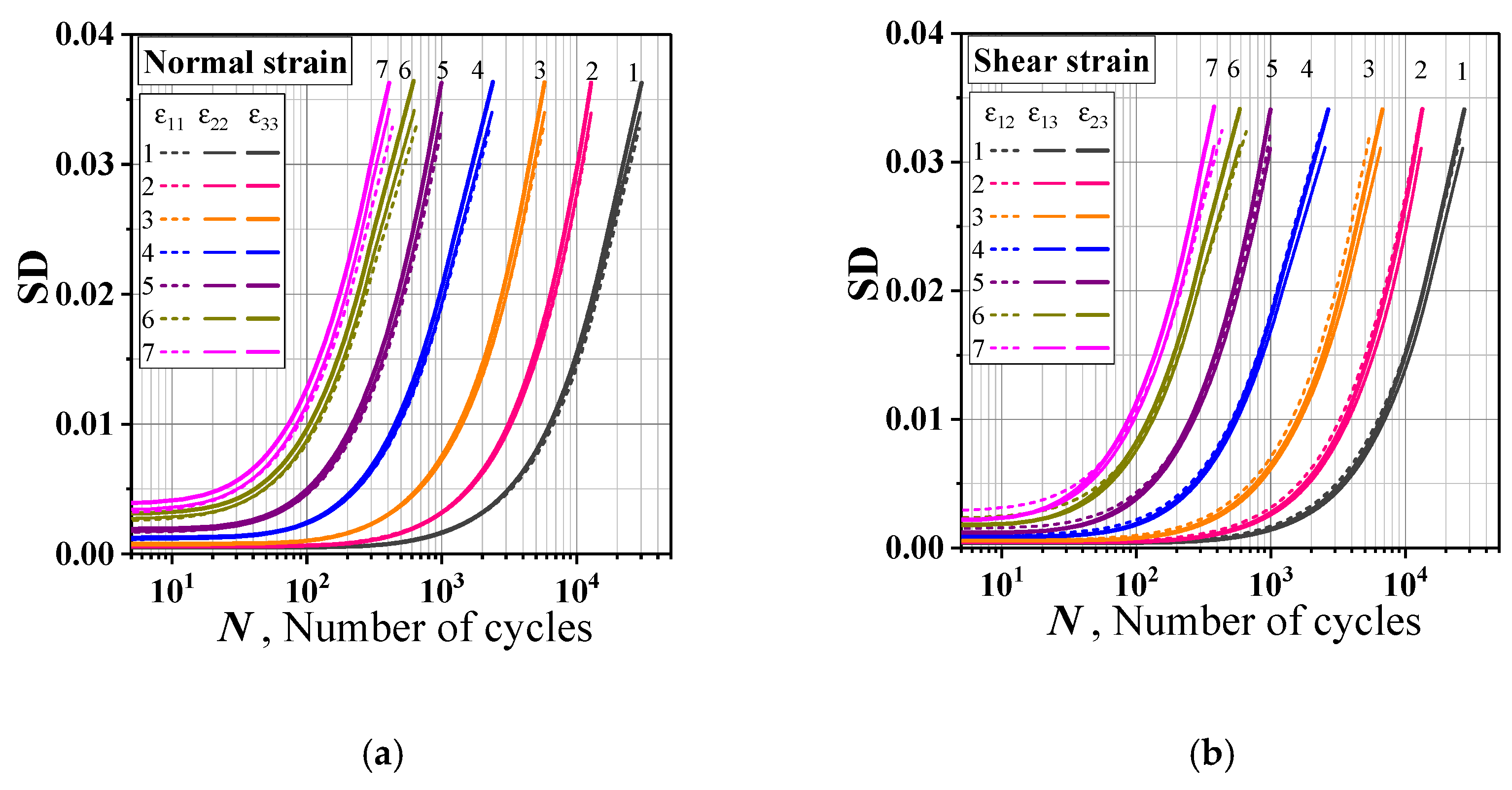
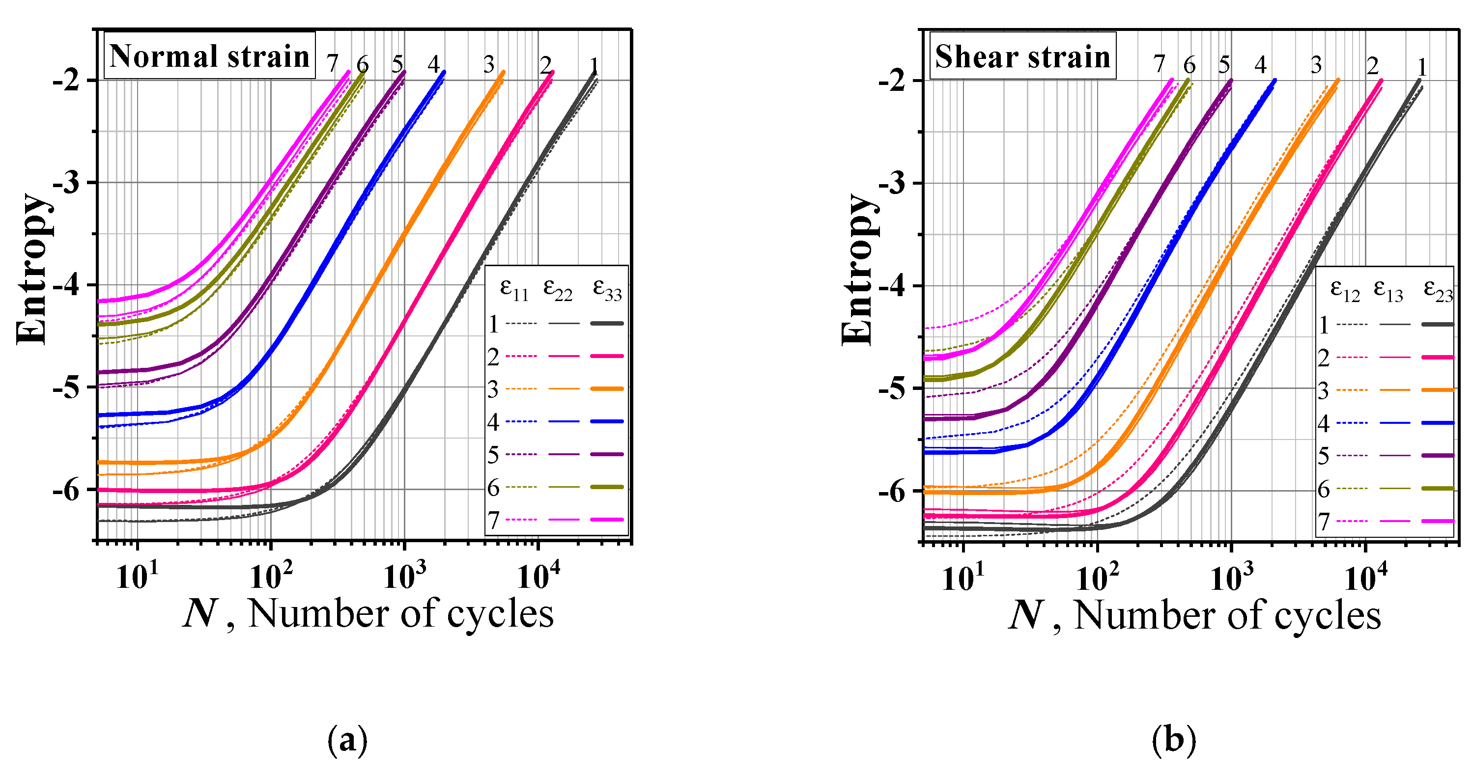
- At grain level, the standard deviation and differential entropy of the respective strain tensor component increase monotonously with the cycle. The standard deviation values of each strain component are almost the same, and the law of their growth with the increase in cycle number is similar. The values of components of differential entropy are close to each other, and the law of that with the number of cycles is also similar.
- (2)
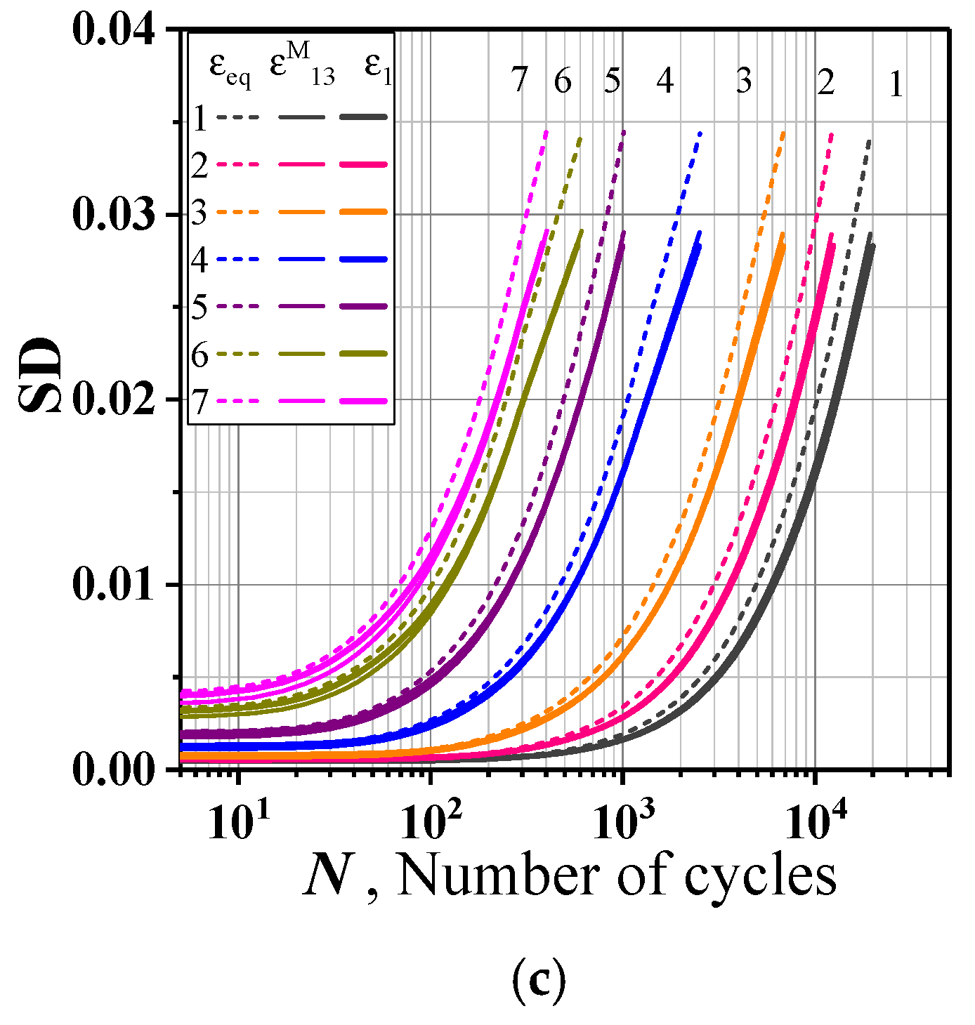
- The respective standard deviations of the effective strain , first principal strain and maximum principal shear strain are similar in numerical and growth law with the number of cycles.
- (3)
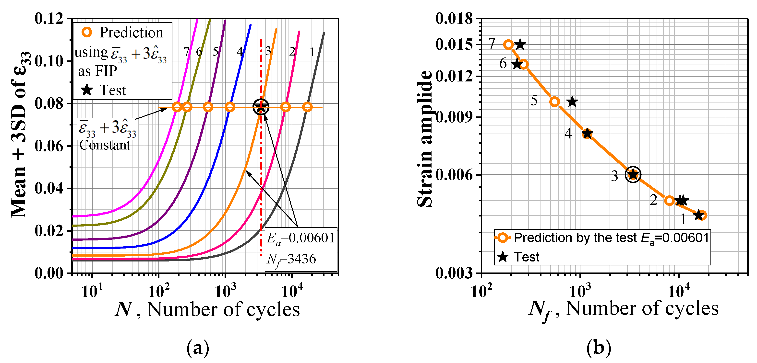
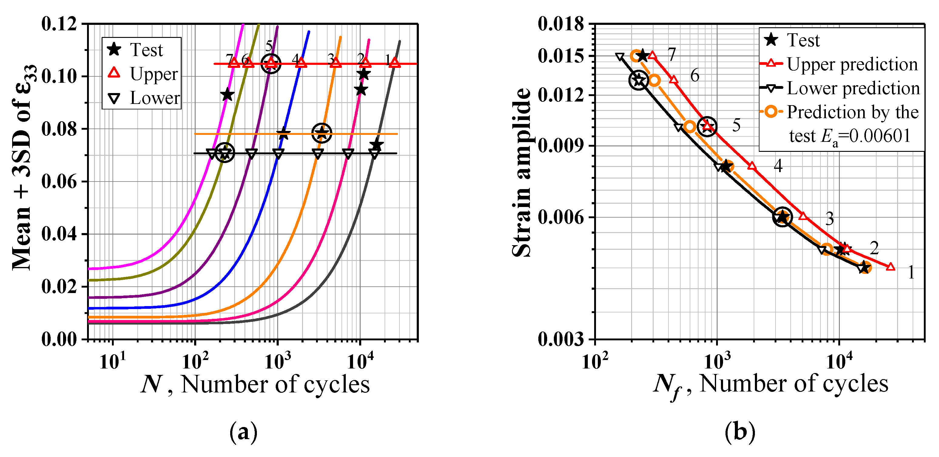
- The parameters ,,, and can be used as fatigue index parameters, and the corresponding critical values can be determined by a single strain amplitude cycle fatigue test, based on which the fatigue–life curve can be predicted.
Author Contributions
Funding
Institutional Review Board Statement
Informed Consent Statement
Data Availability Statement
Acknowledgments
Conflicts of Interest
References
- Stephens, R.I.; Fatemi, A.; Stephens, R.R.; Fuchs, H.O. Cyclic deformation and the strain-life (ε-N) approach. In Metal Fatigue in Engineering, 2nd ed.; Stephens, R.I., Fatemi, A., Stephens, R.R., Fuchs, H.O., Eds.; John Wiley & Sons, Inc.: New York, NY, USA, 2001; pp. 93–121. [Google Scholar]
- Ulewicz, R.; Nový, F.; Novák, P.; Palček, P. The investigation of the fatigue failure of passenger carriage draw-hook. Eng. Fail. Anal. 2019, 104, 609–616. [Google Scholar] [CrossRef]
- Sarkar, P.P.; De, P.S.; Dhua, S.K.; Chakraborti, P.C. Strain energy based low cycle fatigue damage analysis in a plain C-Mn rail steel. Mater. Sci. Eng. A 2017, 707, 125–135. [Google Scholar] [CrossRef]
- Mroziński, S. Energy-based method of fatigue damage cumulation. Int. J. Fatigue 2019, 121, 73–83. [Google Scholar] [CrossRef]
- Chaboche, J.L.; Kanouté, P.; Azzouz, F. Cyclic inelastic constitutive equations and their impact on the fatigue life predictions. Int. J. Plasticity 2012, 35, 44–66. [Google Scholar] [CrossRef]
- Naderi, M.; Hoseini, S.H.; Khonsari, M.M. Probabilistic simulation of fatigue damage and life scatter of metallic components. Int. J. Plasticity 2013, 43, 101–115. [Google Scholar] [CrossRef]
- Sistaninia, M.; Niffenegger, M. Prediction of damage-growth based fatigue life of polycrystalline materials using a microstructural modeling approach. Int. J. Fatigue 2014, 66, 118–126. [Google Scholar] [CrossRef]
- Ma, S.; Yuan, H. A continuum damage model for multi-axial low cycle fatigue of porous sintered metals based on the critical plane concept. Mech. Mater. 2017, 104, 13–25. [Google Scholar] [CrossRef]
- Tanaka, K.; Mura, T. A dislocation model for fatigue crack initiation. J. Appl. Mech. 1981, 48, 97–103. [Google Scholar] [CrossRef]
- Steglich, D.A.; Pirondi, A.N.; Bonora, N.; Brocks, W. Micromechanical modelling of cyclic plasticity incorporating damage. Int. J. Solids Struct. 2005, 42, 337–351. [Google Scholar] [CrossRef]
- Kramberger, J.; Jezernik, N.; Göncz, P.; Glodež, S. Extension of the Tanaka–Mura model for fatigue crack initiation in thermally cut martensitic steels. Eng. Fract. Mech. 2010, 77, 2040–2050. [Google Scholar] [CrossRef]
- Briffod, F.; Shiraiwa, T.; Enoki, M. Microstructure modeling and crystal plasticity simulations for the evaluation of fatigue crack initiation in α-iron specimen including an elliptic defect. Mater. Sci. Eng. A 2017, 695, 165–177. [Google Scholar] [CrossRef]
- Cheong, K.S.; Busso, E.P. Effects of lattice misorientations on strain heterogeneities in FCC polycrystals. J. Mech. Phys. Solids 2006, 54, 671–689. [Google Scholar] [CrossRef]
- Dunne, F.P.E.; Wilkinson, A.J.; Allen, R. Experimental and computational studies of low cycle fatigue crack nucleation in a polycrystal. Int. J. Plasticity 2007, 23, 273–295. [Google Scholar] [CrossRef]
- Wan, V.V.C.; Jiang, J.; MacLachlan, D.W.; Dunne, F.P.E. Microstructure-sensitive fatigue crack nucleation in a polycrystalline Ni superalloy. Int. J. Fatigue 2016, 90, 181–190. [Google Scholar] [CrossRef]
- Dabiri, M.; Lindroos, M.; Andersson, T.; Afkhami, S.; Laukkanen, A.; Björk, T. Utilizing the theory of critical distances in conjunction with crystal plasticity for low-cycle notch fatigue analysis of S960 MC high-strength steel. Int. J. Fatigue 2018, 117, 257–273. [Google Scholar] [CrossRef]
- Farooq, H.; Cailletaud, G.; Forest, S.; Ryckelynck, D. Crystal plasticity modeling of the cyclic behavior of polycrystalline aggregates under non-symmetric uniaxial loading: Global and local analyses. Int. J. Plasticity 2020, 126, 102619. [Google Scholar] [CrossRef] [Green Version]
- Li, D.F.; Barrett, R.A.; O’Donoghue, P.E.; O’Dowd, N.P.; Leen, S.B. A multi-scale crystal plasticity model for cyclic plasticity and low-cycle fatigue in a precipitate-strengthened steel at elevated temperature. J. Mech. Phys. Solids 2017, 101, 44–62. [Google Scholar] [CrossRef] [Green Version]
- Ling, C.; Forest, S.; Besson, J.; Tanguy, B.; Latourte, F. A reduced micromorphic single crystal plasticity model at finite deformations. Application to strain localization and void growth in ductile metals. Int. J. Solids Struct. 2018, 134, 43–69. [Google Scholar] [CrossRef]
- Shi, C.S.; Zeng, B.; Liu, G.L.; Zhang, K.S. Remaining life assessment for steel after low-cycle fatigue by surface crack image. Materials 2019, 12, 823. [Google Scholar] [CrossRef] [PubMed] [Green Version]
- Basaran, C.; Nie, S. An irreversible thermodynamic theory for damage mechanics of solids. Int. J. Damage Mech. 2004, 13, 205–224. [Google Scholar] [CrossRef]
- Egner, W.; Sulich, P.; Mroziński, S.; Egner, H. Modeling thermo-mechanical cyclic behavior of P91 steel. Int. J. Plasticity 2020, 135, 102820. [Google Scholar] [CrossRef]
- Wang, J.D.; Yao, Y. An Entropy-Based Failure Prediction Model for the Creep and Fatigue of Metallic Materials. Entropy 2019, 21, 1104. [Google Scholar] [CrossRef] [Green Version]
- Naderi, M.; Amiri, M.; Khonsari, M.M. On the thermodynamic entropy of fatigue fracture. Proc. R. Soc. A 2010, 466, 423–438. [Google Scholar] [CrossRef] [Green Version]
- Yun, H.; Modarres, M. Measures of Entropy to Characterize Fatigue Damage in Metallic Materials. Entropy 2019, 21, 804. [Google Scholar] [CrossRef] [Green Version]
- Young, C.; Subbarayan, G. Maximum Entropy Models for Fatigue Damage in Metals with Application to Low-Cycle Fatigue of Aluminum 2024-T351. Entropy 2019, 21, 967. [Google Scholar] [CrossRef] [Green Version]
- Sweeney, C.A.; O’Brien, B.; Dunne, F.P.E.; McHugh, P.E.; Leen, S.B. Strain-gradient modelling of grain size effects on fatigue of CoCr alloy. Acta Mater. 2014, 78, 341–353. [Google Scholar] [CrossRef]
- Cruzado, A.; Lucarini, S.; LLorca, J.; Segurado, J. Microstructure-based fatigue life model of metallic alloys with bilinear Coffin-Manson behavior. Int. J. Fatigue 2018, 107, 40–48. [Google Scholar] [CrossRef] [Green Version]
- Lucarini, S.; Segurado, J. An upscaling approach for micromechanics based fatigue: From RVEs to specimens and component life prediction. Int. J. Fract. 2020, 223, 93–108. [Google Scholar] [CrossRef]
- Zhang, K.S.; Shi, Y.K.; Ju, J.W. Grain-level statistical plasticity analysis on strain cycle fatigue of a fcc metal. Mech. Mater. 2013, 64, 76–90. [Google Scholar] [CrossRef]
- Zhang, K.S.; Ju, J.W.; Li, Z.; Bai, Y.L.; Brocks, W. Micromechanics based fatigue life prediction of a polycrystalline metal applying crystal plasticity. Mech. Mater. 2015, 85, 16–37. [Google Scholar] [CrossRef] [Green Version]
- Zhang, M.H.; Shen, X.H.; He, L.; Zhang, K.S. Application of differential entropy in characterizing the deformation inhomogeneity and life prediction of low-cycle fatigue of metals. Materials 2018, 11, 1917. [Google Scholar] [CrossRef] [PubMed] [Green Version]
- Wu, X.R.; Yang, S.J.; Han, X.P.; Liu, S.L.; Liu, Q.S.; Lu, K.R.; Li, J.N.; Guan, H.R.; Feng, D. Data Manual for Materials of Aero-Engine, Aircraft Engine Design Data Manual for Materials; Aviation Industry Press: Beijing, China, 2008. (In Chinese) [Google Scholar]
- Li, H.Y.; Kong, Y.H.; Chen, G.S.; Xie, L.X.; Zhu, S.G.; Sheng, X. Effect of different processing technologies and heat treatments on the microstructure and creep behavior of GH4169 superalloy. Mater. Sci. Eng. A 2013, 582, 368–373. [Google Scholar] [CrossRef]
- Hill, R.; Rice, J.R. Constitutive analysis of elastic-plastic crystal at arbitrary strain. J Mech Phys Solids 1972, 20, 401–413. [Google Scholar] [CrossRef]
- Asaro, R.J.; Rice, J.R. Strain localization in ductile single crystals. J. Mech. Phys. Solids 1977, 25, 309–338. [Google Scholar] [CrossRef] [Green Version]
- Peirce, D.; Asaro, R.J.; Needleman, A. Material rate dependence and localized deformation in crystalline solids. Acta Metall. 1983, 31, 1951–1976. [Google Scholar] [CrossRef]
- Hutchinson, J.W. Bounds and self-consistent estimates for creep of polycrystalline materials. Proc. R. Soc. Lond. Ser. A 1976, 348, 101–127. [Google Scholar]
- Feng, L.; Zhang, G.; Zhang, K.S. Discussion of cyclic plasticity and viscoplasticity of single crystal nickel-based superalloy in large strain analysis: Comparison of anisotropic macroscopic model and crystallographic model. Int. J. Mech. Sci. 2004, 46, 1157–1171. [Google Scholar]
- Pan, J.; Rice, J.R. Rate sensitivity of plastic flow and implications for yield-surface vertices. Int. J. Solids Struct. 1983, 19, 973–987. [Google Scholar] [CrossRef] [Green Version]
- Hutchinson, J.W. Elastic-plastic behaviour of polycrystalline metals and composites. Proc. R. Soc. Lond. Ser. A 1970, 319, 247–272. [Google Scholar]
- Chang, Y.W.; Asaro, R.J. An experimental study of shear localization in aluminum-copper single crystals. Acta Metall. 1981, 29, 241–257. [Google Scholar] [CrossRef]
- Shannon, C.E.; Weaver, W. The Mathematical Theory of Communication; University of Illinois Press: Champaign, IL, USA, 1964; pp. 81–108. [Google Scholar]


| Elastic Constants | Material Parameters of the Crystal Plasticity Model | ||||||||||||
|---|---|---|---|---|---|---|---|---|---|---|---|---|---|
| C11 | C12 | C44 | τ0 | τs | h0 | a | c | λ | e1 | e2 | q | k | |
| GPa | GPa | GPa | MPa | MPa | MPa | GPa | GPa | s−1 | s−1 | ||||
| 230.05 | 153.57 | 81.97 | 289 | 295 | 80 | 59 | 0.428 | 0 | 0 | 0 | 1 × 10⁻³ | 1 | 160 |
| Ea | 0.0045 | 0.005 | 0.00601 | 0.00801 | 0.01003 | 0.01306 | 0.015 |
|---|---|---|---|---|---|---|---|
| Nf, Cycles | 15,855 | 10,289/11,087 | 3436 | 1181 | 811 | 229 | 246 |
Publisher’s Note: MDPI stays neutral with regard to jurisdictional claims in published maps and institutional affiliations. |
© 2021 by the authors. Licensee MDPI, Basel, Switzerland. This article is an open access article distributed under the terms and conditions of the Creative Commons Attribution (CC BY) license (http://creativecommons.org/licenses/by/4.0/).
Share and Cite
Zhang, M.-H.; Shen, X.-H.; He, L.; Zhang, K.-S. Investigation of Deformation Inhomogeneity and Low-Cycle Fatigue of a Polycrystalline Material. Appl. Sci. 2021, 11, 2673. https://doi.org/10.3390/app11062673
Zhang M-H, Shen X-H, He L, Zhang K-S. Investigation of Deformation Inhomogeneity and Low-Cycle Fatigue of a Polycrystalline Material. Applied Sciences. 2021; 11(6):2673. https://doi.org/10.3390/app11062673
Chicago/Turabian StyleZhang, Mu-Hang, Xiao-Hong Shen, Lei He, and Ke-Shi Zhang. 2021. "Investigation of Deformation Inhomogeneity and Low-Cycle Fatigue of a Polycrystalline Material" Applied Sciences 11, no. 6: 2673. https://doi.org/10.3390/app11062673