Uniformity, Periodicity and Symmetry Characteristics of Forces Fluctuation in Helical-Edge Milling Cutter

Abstract

Under most processing conditions, the milling force is expected to be stable and not to fluctuate, in order to improve the processing quality. This study focuses on analyzing the force fluctuation characteristics under conditions of different processing and cutter parameters. An original model is proposed to predict the force fluctuation during the milling process of a helical-edge cutter. At the same time, three force fluctuation characteristics related to the axial cutting depth and cutter parameters are determined: uniformity, periodicity and symmetry. The corresponding mathematical derivation and proof method are given for the first time through a force transformation of projecting the superposition chip thickness on a virtual cutting edge. On this basis, a fast estimation method and an accurate simulation method for force fluctuation prediction are established to quantify the intensity of force fluctuations under different parameters. Both two prediction methods and the experimental cutting tests validate the proposed theory effectively. The result shows a high potential of the proposed theory for studying the force behavior under different milling parameters or cutter parameters and at least 75% of the test workload can be reduced.

1. Introduction

The milling cutter of a helical-edge has been widely used in high-speed and high-precision manufacturing, especially in side milling. The ever-changing interaction between the helical edge and workpiece causes the milling force to fluctuate rapidly and complexly, which has a great influence on machining quality and efficiency [1]. Therefore, the force fluctuation characteristics were studied and used as an indicator, such as tool wear [2], surface quality [3,4] and parameter monitoring [5]. In order to avoid the effect of force fluctuations in the high-speed and high-precision milling, a small cutting width or depth should be used, while feed speed and other processing parameters should be reduced [6,7,8]. However, this reduces productivity and limits the potential processing improvement. To this end, studying the force generation mechanism of a helical-edge cutter and revealing the force fluctuation behavior in high-speed and high-precision machining have great research value.

Most of the studies on the milling force are based on the force prediction model proposed by Altintas [9,10,11]. The most representative theoretical modeling method is to apply the oblique cutting theory. The force of the milling cutter can be dispersed into a series of micro-elements along the axial direction, where each micro-element is considered as an oblique cutting process. Then, the milling force can be calculated by force superimposed on each micro-element. Accordingly, the study of milling force can be divided into two parts. The first one is the research on the supplement of a milling force model [12,13,14]. The related literature shows that many enhanced force models have been proposed and they have been mainly focused on improving the accuracy and the scope of the application [15,16]. However, although the force fluctuation in the milling process is also a very important characteristic, the existing milling force models lack a good description of force fluctuation characteristics. This study supplements the force model description from the mentioned aspect. Another part is the study on the milling force model to reveal the influence of different parameters on force fluctuation characters. The parameters can be roughly divided into two categories: cutter parameters and processing parameters [17,18]. Jiang [19] studied the influence of the mentioned parameters on the milling force, such as cutter geometrical parameters (helix angle and rake angle) and milling parameters (axial depth of cut, radial depth of cut, feed rate per tooth and cutting speed. The research results showed that the axial depth of cut, radial depth of cut and cutter helix angle were the main affecting factors of the engagement angle of the milling force. In addition, Sahoo, P. and Pimenov, D.Y. [20] considered the influence of tool runout, minimum chip thickness, elastic recovery, ploughing area, entry and exit angles. Liu [21] supplemented the study of the edge number parameter and the cutter diameter parameter and pointed out that an ideal force distribution should be as continuous as possible. The ideal selection of the cutter and processing parameters can not only reduce the surface error, but also make it possible to achieve a high finishing accuracy in semi-finishing. Although the previous studies have considered the effects of individual changes in each parameter on force characteristics, the mathematical relationship between various parameters and the intensity of milling force fluctuation, such as combined changes in the axial depth of cut, helix angle and tool radius, have still not been revealed and explained clearly.

After years of research, scholars aimed to summarize the characteristics and rules of force fluctuations and tried to define a comprehensive theorem. Yang [22] studied the relationship between the characteristics of the milling force curve, axial depth of cut, radial depth of cut and helix angle. The force fluctuations were classified into three types according to angular distance PT_doc (PT_doc is the force valley and the force peak that followed). Arshinov and Alekseev [23] proposed a uniformity theory and it was pointed out that the uniformity of the cutting force fluctuation curve would occur when the milling cutter had helical edges. Huang [24] completed the mathematical derivation of the uniformity theory and put forward the periodicity theory. It was proven that the milling force changed periodically with the change in the axial cutting depth. However, the research on milling force fluctuation has still not been comprehensive and there are more characteristics that need to be studied further.

In this paper, a new symmetry theory is introduced to study the milling force fluctuation characteristics of a helical-edge milling cutter. In addition, the mathematical derivations of uniformity, periodicity and symmetry characteristics are proven using a force transformation method of a virtual cutting edge projection. The experimental results verify that the proposed theory can reveal the force fluctuation characteristics. Furthermore, it is shown that when the proposed theory is applied, the milling test needs only 25% of the axial depth of cut to reveal the characteristics of force fluctuation at all cut depths. This proves that the proposed theory can significantly reduce the test workload in a milling force experiment and can also be used in the experimental research of milling force behavior.

The rest of the paper is organized as follows. Section 2 presents research prerequisites and derives the force fluctuation formula based on the oblique cutting theory. Section 3 puts forward a concept of a virtual edge. Using the equivalent change in the milling force model, the milling force of each edge can be translated and superimposed on the virtual edge. Hence, the three characteristics of milling force fluctuation are presented and proven by mathematical derivations. To quantify the intensity of force fluctuations under different parameters, Section 4 introduces two prediction methods: a fast estimation method and an accurate simulation method. The error between the two methods is verified by experiments. Then, another illustrative experiment is conducted to validate the proposed theory. Section 5 concludes the paper and presents future work directions.

2. Milling Force Fluctuation Mechanism of Helical-Edge Cutter

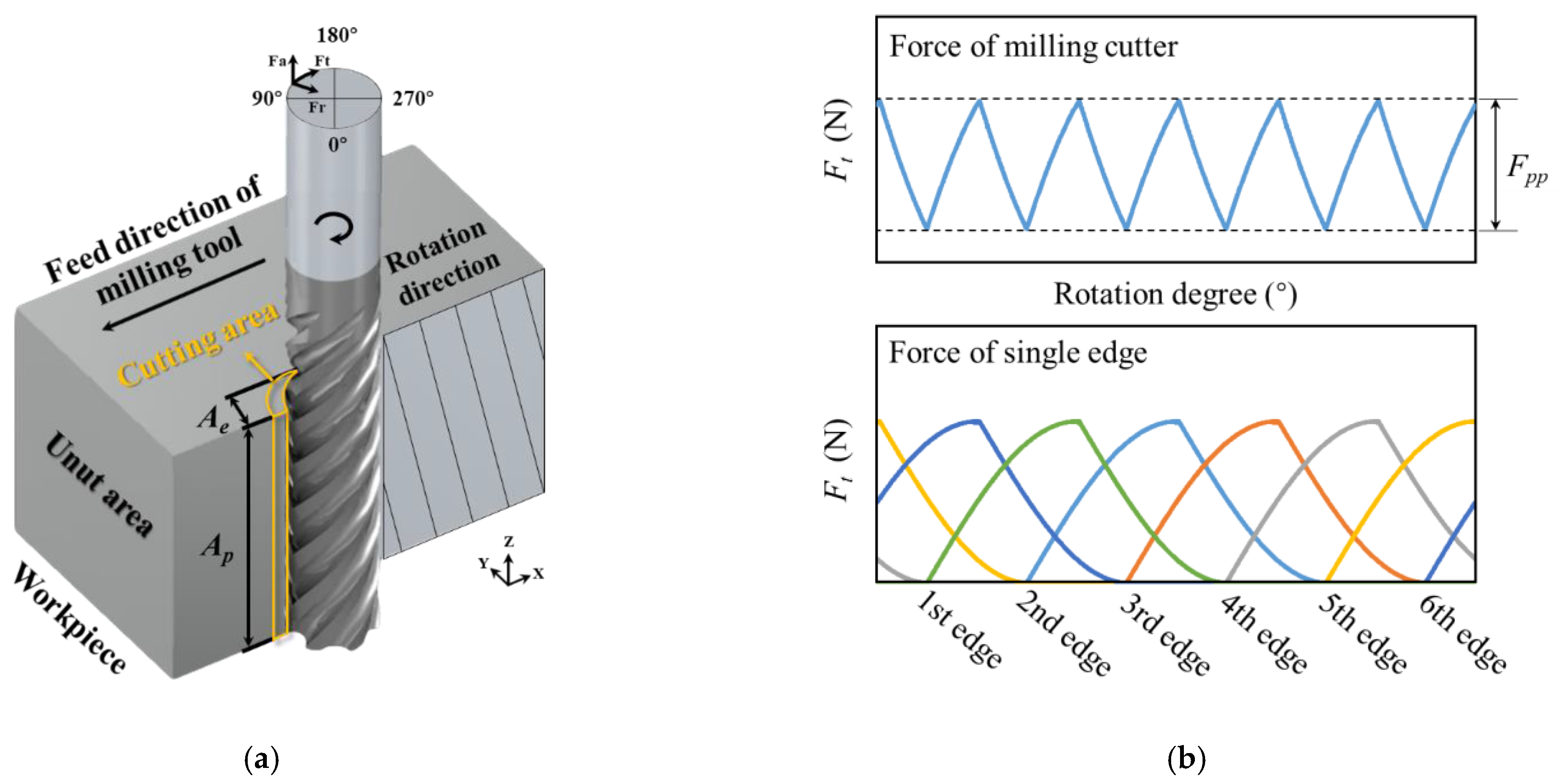
2.1. Milling Process and Theory Preconditions

A helical-edge cutter performs a unique milling process where every cutting edge removes material from a workpiece gradually and continuously. Therefore, the milling force caused by each cutting edge continuously fluctuates from minimum to maximum value. The milling geometry and mechanism of a helical-edge cutter are presented in Figure 1. The geometry of a down-milling process and related parameters are shown in Figure 1a. The machine tool and workpiece share the same x-y-z coordinate system, while the milling cutter uses the t-r-a coordinate system. The milling cutter feeds along the negative x-direction and rotates clockwise from zero to 360°. The force generated by the rotation of the milling cutter is presented in Figure 1b. As mentioned previously, due to the unique milling mechanism caused by the helix angle, the force generated by each edge is continuous and periodic. Hence, the fluctuation force of the milling cutter obtained by the superposition of the forces generated by all edges is also periodic and continuous. This provides a theoretical possibility to reveal and summarize the force fluctuation characteristics F_pp (the peak-to-peak value of the milling force). In order to simplify the research process, this study adopts the following preconditions:

• The milling process is general and simple, which means the influences of the tool wear, deformation, runout and chatter are not considered;
• The milling force model is widely accepted [9]. In this model, the tool path is considered as a circle when calculating the chip thickness. The cutting force caused by the size effect coefficients (K_tc, K_rc, K_ac) is considered as the main factor and the ploughing effect is ignored in side milling;
• The processing parameters are smooth and not extreme. Under this condition, the milling force coefficient is stable and can be considered as an average value.

2.2. Milling Process and Theory Preconditions

To define the general form of the force fluctuation model, the basic milling force model is used based on the oblique cutting theory. The total milling force of a helical-edge cutter is calculated by superimposing the forces of all its micro-elements. As shown in Figure 2, the cutting area is equally divided along the axial direction. According to the accuracy requirement, the height of each micro-element is set to ΔZ. Then, the force components of each micro-element in the three directions are expressed as follows [9]:

$$\{\begin{array}{c}{F}_t\left({\theta }_{i,j}\right)=K_{tc}{f}_{t}sin({\theta }_{i,j})g\left({\theta }_{i,j}\right)\Delta Z\hfill \\ F_r\left({\theta }_{i,j}\right)=K_{rc}{f}_{t}sin({\theta }_{i,j})g\left({\theta }_{i,j}\right)\Delta Z\hfill \\ F_a\left({\theta }_{i,j}\right)=K_{ac}{f}_{t}sin({\theta }_{i,j})g\left({\theta }_{i,j}\right)\Delta Z\hfill \end{array}$$

(1)

where, F_t, F_r, F_a are tangential, radial and axial cutting forces, respectively. K_tc, K_rc, K_ac are tangential, radial and axial cutting force coefficients, respectively. The variable f_t is the feed per tooth and g(θ) is a judgment function to determine whether the micro-element is in milling.

$$\Delta Z=\frac{A_p}{N_d},$$

(2)

$$g\left({\theta }_{i,j}\right)=\{\begin{array}{cc}1,& {\theta }_{st}\le {\theta }_{i,j}\le {\theta }_{ex}\\ 0,& Others\end{array},$$

(3)

$${\theta }_{st}=\{\begin{array}{cc}\pi & ,up milling\\ \pi -arccos(1-\frac{A_e}{R})& ,down milling\end{array},$$

(4)

$${\theta }_{ex}=\{\begin{array}{cc}\pi +arccos(1-\frac{A_e}{R})& ,up milling\\ \pi & ,down milling\end{array}.$$

(5)

where, ΔZ is height of a micro-element in the z-direction. A_e and A_p are radial and axial depths of cut, respectively. θ_st and θ_ex are entrance and exit angle, respectively. N_d is the total number of axial micro-elements. R is the radial of a cutting tool.

In order to calculate the force fluctuation, an initial angle is set as a reference point. Assuming that the lowest element of the first edge is regarded as a reference point θ₀, angle θ_i,j can be expressed as:

$${\theta }_{i,j}={\theta }_0-\frac{2\pi }{N_t}\times \left(j-1\right)-\frac{tan\beta }{R}\times \left(i-\Delta Z\right).$$

(6)

where i is the current height of the micro-elements in the z-direction, j is the cutting edge index, θ_i,j is the tool rotating angle of a tooth j at a height I, β is the helix angle of a cutter and N_t is the total number of cutting edges.

By substituting Equations (3)–(6) into Equation (1), the total milling force can be obtained as:

$$\begin{gathered} \left[\begin{array}{c}{F}_t\\ F_r\\ F_a\end{array}\right]=\left[\begin{array}{c}{K}_{tc}\\ K_{rc}\\ K_{ac}\end{array}\right]\times {\displaystyle \sum }_{j=1}^{N_t}{\displaystyle \sum }_{i=\Delta Z}^{A_p}{f}_t\times sin\left({\theta }_0-\frac{2\pi }{N_t}\times \left(j-1\right)-\frac{tan\beta }{R}\times \left(i-\Delta Z\right)\right)\times \Delta Z \\ \left(\pi -arccos(1-\frac{A_e}{R}\right)\le \left({\theta }_0-\frac{2\pi }{N_t}\times \left(j-1\right)-\frac{tan\beta }{R}\times \left(i-\Delta Z\right)\right)\le \pi ). \end{gathered}$$

(7)

In order to analyze the force behavior under different cutter rotation angles and axial depth of cut, Equation (7) is deformed to facilitate the study.

$$F\left({\theta }_0,A_p\right)=KC{\displaystyle \sum }_{j=1}^{N_t}{\displaystyle \sum }_{i=\Delta Z}^{A_p}G\left({\theta }_0-\frac{2\pi }{N_t}\times \left(j-1\right)-\frac{tan\beta }{R}\times \left(i-\Delta Z\right)\right)$$

(8)

where, $F\left({\theta }_0,A_p\right)=\left[\begin{array}{c}{F}_t\left({\theta }_0,A_p\right)\\ F_r\left({\theta }_0,A_p\right)\\ F_a\left({\theta }_0,A_p\right)\end{array}\right]$, $K=\left[\begin{array}{c}{K}_{tc}\\ K_{rc}\\ K_{ac}\end{array}\right]$, $C=f_z \Delta Z$, $G\left(\theta \right)=\{\begin{array}{cc}sin\left(\theta \right),\hfill & {\theta }_{st}\le \theta \le {\theta }_{ex}\\ 0,\hfill & Others\end{array}$.

Finally, the milling force fluctuation characteristics, which can be expressed as the peak-to-peak value of the milling force (F_pp), can be deduced as:

$$F_{pp}\left(A_p\right)=\mathrm{Max}\left\{F\left({\theta }_0,A_p\right)\right\}-\mathrm{Min}\left\{F\left({\theta }_0,A_p\right)\right\},\left({\theta }_0\subseteq \left[0^{°},{360}^{°}\right]\right).$$

(9)

3. Milling Force Fluctuation Characteristics

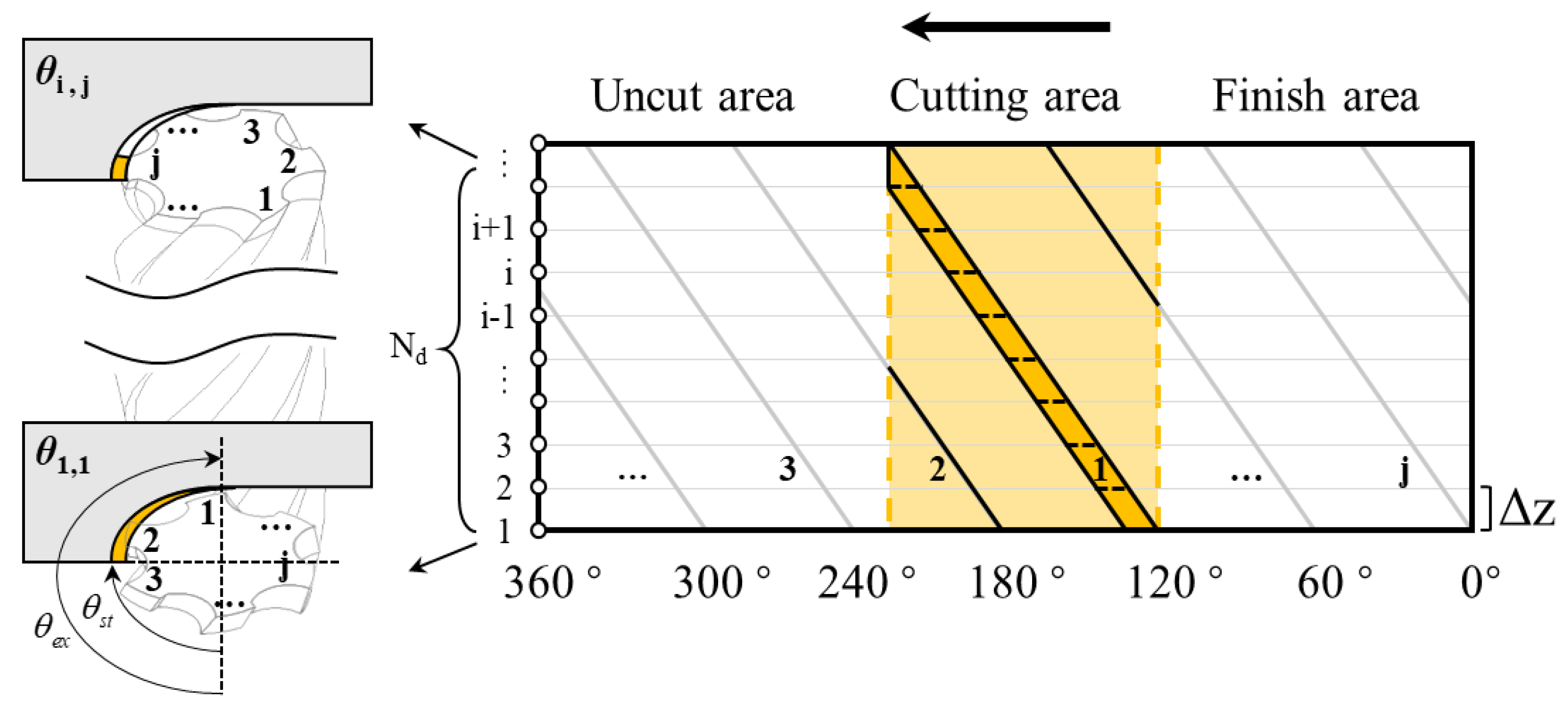
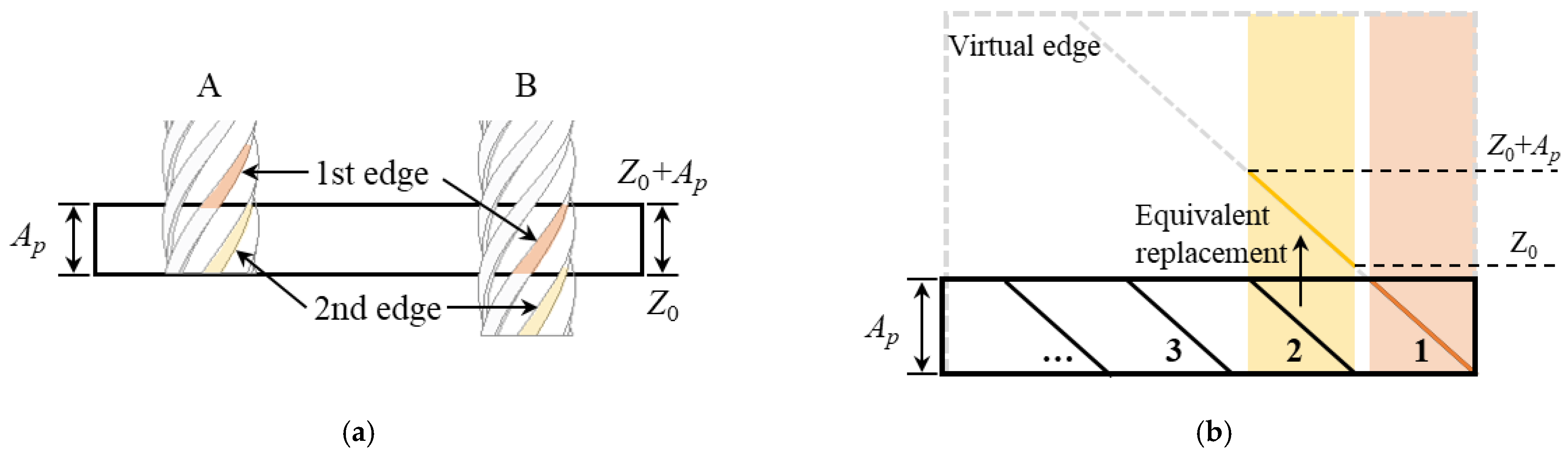
3.1. Virtual-Edge Projection Method of Force Equation Transformation

In order to identify the force behavior under different milling positions and rotation angles, a virtual-edge projection method is proposed to reveal the force relationship between each cutting edge. This method is based on the physical phenomenon that if the cutter edge is long enough, each cutting edge can be replaced by the previous edge above it, as shown in Figure 3. In Figure 3a, two milling cutters denoted as A and B have different milling positions and their axial cutting depth is A_p. The difference between cutters A and B is that the milling position of cutter A is from zero to A_p and that of cutter B is from Z₀ to (Z₀ + A_p), where Z₀ is an axial offset reference position, defined as follows:

During the milling process, if an edge is in contact with the workpiece, then move the milling cutter downwards axially until the previous edge reaches the same position, the axial offset of this downward movement is defined as Z₀.

The milling forces caused by a single edge of the two cutters are analyzed for comparison. The milling force expression of the second cutting edge of cutter A can be calculated by Equation (8) as follows:

$$F_{A2}\left({\theta }_0,A_p\right)=KC{\displaystyle \sum }_{i=\Delta Z}^{A_p}G\left({\theta }_0-\frac{2\pi }{N_t}-\frac{tan\beta }{R}\times \left(i-\Delta Z\right)\right)$$

(10)

At the same time, the corresponding milling force expression of the first edge of cutter B is calculated by:

$$F_{B1}\left({\theta }_0,A_p\right)=KC{\displaystyle \sum }_{i=Z_0+\Delta Z}^{Z_0+Ap}G\left({\theta }_0-\frac{tan\beta }{R}\times \left(i-\Delta Z\right)\right)$$

(11)

Considering that in Equations (10) and (11) the rotation reference point θ₀ is the same, the following Equation (12) can be obtained:

$$\begin{array}{c}{F}_{A2}\left({\theta }_0,A_p\right)=KC{\displaystyle \sum _{i=\Delta Z}^{A_p}}G\left({\theta }_0-\frac{2\pi }{N_t}-\frac{tan\beta }{R}\times \left(i-\Delta Z\right)\right)\hfill \\ =KC{\displaystyle \sum _{i=\Delta Z}^{A_p}}G\left({\theta }_0-\frac{2\pi }{N_t}+\frac{tan\beta }{R}\times Z_0-\frac{tan\beta }{R}\times \left(i-\Delta Z\right)-\frac{tan\beta }{R}\times Z_0\right)\hfill \\ =KC{\displaystyle \sum _{i=Z_0+\Delta Z}^{Z_0+Ap}}G\left({\theta }_0-\frac{2\pi }{N_t}+\frac{tan\beta }{R}\times Z_0-\frac{tan\beta }{R}\times \left(i-\Delta Z\right)\right)\hfill \\ =F_{B1}\left({\theta }_0-\frac{2\pi }{N_t}+\frac{tan\beta }{R}\times Z_0,A_p\right).\end{array}$$

(12)

Therefore, based on Equation (12), the following conclusion can be drawn. The movement of the axial milling position can be compensated by the rotation angle of a cutter. If Equation (12) is transformed, then the following equations can be obtained:

$$\{\begin{array}{c}{F}_{A2}\left({\theta }_0,A_p\right)=F_{B1}\left({\theta }_0,A_p\right)\hfill \\ Z_0=\frac{2\pi R}{N_{t}tan\beta }\hfill \end{array}.$$

(13)

Equation (13) illustrates that the milling force of each edge from zero to A_p can be replaced by the force of the previous edge from Z₀ to Z₀ + A_p. Therefore, as shown in Figure 3b, if there is an infinitely long virtual edge along the first edge, the milling force of the other edges can always be represented by a specific part of the virtual edge. This virtual-edge projection method provides a more intuitive graphical representation for the mathematical expression of the milling force.

3.2. Uniformity Characteristics of Force Fluctuation

There is a special milling situation in the milling process of a helical-fluent cutter. Namely, when the first cutting edge gradually exits the workpiece, then the next cutting edge gradually enters the workpiece. Also, the length and thickness of the cutting edge are not changed. Therefore, the milling force will be constant and F_pp will be zero. This phenomenon is called the uniformity milling process and it is presented in Figure 4. The uniformity milling process is greatly affected by the entrance and exit angles. According to Equation (13), the parameters that affect these two angles are A_e, A_p, R, N_t and β. As mentioned in Section 3.1., if the cutting depth of the milling process is A_p, the projection range of the first edge on the virtual edge is from zero to A_p and the range of the second edge is from Z₀ to (Z₀ + A_p). Therefore, if A_p is equal to Z₀, then the projection range of the virtual edge is continuous. This means that the milling force is stable and is no longer affected by the rotation angle and radial depth of the cut. Accordingly, A_p is defined as A_poc, which represents one-cycle of axial depth of cut and is expressed as:

$$A_{poc}=\frac{2\pi R}{N_{t}tan\beta }.$$

(14)

The virtual-edge projection of a uniformity milling process is illustrated in Figure 4a. In order to prove the uniformity characteristics of the milling force, it is assumed that the axial cutting depth is A_poc and the radial cutting depth A_e is an arbitrary value. At this time, the calculation of the milling force can be divided into two cases. The first case is that the force projection area is on a single edge and the effective projection area is from Z₁ to (Z₁ + δZ). The other case is that the force projection area exists on multiple edges and the effective projection area is from Z₂ to (Z₂ + δZ). In Figure 4, the effective force projection area A of the first case is displayed in the color orange and the rotation angle is θ_Z1. In the first case, the milling force of the virtual-edge projection area F_ve can be calculated as follows:

$$\begin{array}{c}{F}_A\left({\theta }_{Z_1},A_{poc}\right)=KC{\displaystyle \sum _{i=Z_1+\Delta Z}^{Z_1+\delta Z}}G\left({\theta }_{Z_1}-\frac{tan\beta }{R}\times \left(i-\Delta Z\right)\right)\hfill \\ =KC{\displaystyle \sum _{i=\Delta Z}^{\delta Z}}G\left({\theta }_{Z_1}-\frac{tan\beta }{R}\times Z_1-\frac{tan\beta }{R}\times \left(i-\Delta Z\right)\right)\hfill \\ =F_{ve}\left({\theta }_0,A_{poc}\right).\end{array}$$

(15)

In the second case, the first edge is cutting out of the workpiece and the second edge is cutting in the workpiece; the effective force projection area exists on multiple edges. Then, the effective force projection area B is displayed in the color red and the rotation angle is θ_Z2.

$$\begin{array}{c}{F}_B\left({\theta }_Z{}_2,A_{poc}\right)=KC\left({\displaystyle \sum _{i=Z_2+\Delta Z}^{A_{poc}}}G\left({\theta }_{Z_2}-\frac{tan\beta }{R}\times \left(i-\Delta Z\right)\right)+{\displaystyle \sum _{i=Z_2+\Delta Z}^{A_{poc}}}G\left({\theta }_{Z_2}-\frac{2\pi }{N_z}-\frac{tan\beta }{R}\times \left(i-\Delta Z\right)\right)\right)\hfill \\ =KC\left({\displaystyle \sum _{i=Z_2+\Delta Z}^{A_{poc}}}G\left({\theta }_{Z_2}-\frac{tan\beta }{R}\times \left(i-\Delta Z\right)\right)+{\displaystyle \sum _{i=A_{poc}+\Delta Z}^{Z_2+\delta Z}}G\left({\theta }_{Z_2}-\frac{2\pi }{N_z}+\frac{tan\beta }{R}\times A_{poc}-\frac{tan\beta }{R}\times \left(i-\Delta Z\right)\right)\right)\hfill \\ =KC{\displaystyle \sum _{i=Z_2+\Delta Z}^{Z_2+\delta Z}}G\left({\theta }_{Z_2}-\frac{tan\beta }{R}\times \left(i-\Delta Z\right)\right)\hfill \\ =KC{\displaystyle \sum _{i=\Delta Z}^{\delta Z}}G\left({\theta }_{Z_2}-\frac{tan\beta }{R}\times Z_2-\frac{tan\beta }{R}\times \left(i-\Delta Z\right)\right)\hfill \\ =F_{ve}\left({\theta }_0,A_{poc}\right).\end{array}$$

(16)

Therefore,

$$\{\begin{array}{c}{F}_A\left({\theta }_{Z_1},A_{poc}\right)=F_B\left({\theta }_{Z_2},A_{poc}\right)=F_{ve}\left({\theta }_0,A_{poc}\right)=C_0\hfill \\ F_{pp}\left(A_{poc}\right)=0\hfill \end{array}.$$

(17)

Equation (17) shows that the milling force is a constant value C₀ and does not change with the rotation angle θ; C₀ is defined as the constant force generated by the milling tool at an axial depth of A_poc, where uniformity milling occurs. In addition, three inferences can be deduced:

Inference 1.

As the value of A_e only affects the projection size of δZ, therefore, regardless of the value of A_e, Equation (17) is still applicable, but the value of C₀ is different.

Inference 2.

Since the sum of two constants is also a constant, a conclusion can be drawn that the uniformity characteristics are still available in other cycles, which is expressed as follows:

$$F_{pp}\left(n{A}_{poc}\right)=0,\left(n=1,2,3\dots \right).$$

(18)

Inference 3.

If the axial depth of cut is A_poc, the milling force of F_x, F_y and F_z still have the same characteristics. Since the proof process of Equations (10)–(18) is still same, the subfunction in Equation (8) can be redefined as follows:

$$F\left({\theta }_0,A_p\right)=KC{\displaystyle \sum }_{j=1}^{N_t}{\displaystyle \sum }_{i=\Delta Z}^{A_p}G\left({\theta }_0-\frac{2\pi }{N_t}\times \left(j-1\right)-\frac{tan\beta }{R}\times \left(i-\Delta Z\right)\right)$$

(19)

where if the milling force is in the t-r-a coordinate system,$F\left({\theta }_0,A_p\right)=\left[\begin{array}{c}{F}_t\left({\theta }_0,A_p\right)\\ F_r\left({\theta }_0,A_p\right)\\ F_a\left({\theta }_0,A_p\right)\end{array}\right]$, then$K=\left[\begin{array}{c}{K}_{tc}\\ K_{rc}\\ K_{ac}\end{array}\right]$, $C=f_z\Delta Z$, $G\left(\theta \right)={\{\begin{array}{cc}sin\left(\theta \right),\hfill & {\theta }_{st}\le \theta \le {\theta }_{ex}\\ 0,\hfill & Others\end{array}}_{}$, else if the milling force is in the x-y-z coordinate system,$F\left({\theta }_0,A_p\right)=\left[\begin{array}{c}{F}_t\left({\theta }_0,A_p\right)\\ F_r\left({\theta }_0,A_p\right)\\ F_a\left({\theta }_0,A_p\right)\end{array}\right]$, then,$K= \left[\begin{array}{c}{K}_{tc}\\ K_{rc}\\ K_{ac}\end{array}\right]$, $C=f_z\Delta Z$, $G\left(\theta \right)=\{\begin{array}{cc}\left[\begin{array}{ccc}-sin\left(\theta \right)cos\left(\theta \right)& sin\left(\theta \right)sin\left(\theta \right)& 0\\ sin\left(\theta \right)sin\left(\theta \right)& sin\left(\theta \right)cos\left(\theta \right)& 0\\ 0& 0& 1\end{array}\right],& {\theta }_{st}\le \theta \le {\theta }_{ex}\\ 0,& Others\end{array}$.

Equation (19) extends the definition of the range of the milling force in Equation (8). This makes the force equation not only valid in the t-r-a coordinate system, but also in the x-y-z coordinate system. In the rest of this article, the definition of F(θ₀, A_p) always refers to the definition of F(θ₀, A_p) in Equation (19).

3.3. Periodicity Characteristics of Force Fluctuation

Since the milling force changes periodically to a constant value with nA_poc, as shown in Figure 5, if there exists δA_p such that whatever the δA_p value is, the value of F_pp(δA_p + T) is always equal to the value of F_pp(δA_p), then the milling force fluctuation can be regarded as a periodic function, where T is the period. To prove this theory of periodicity characteristics, an arbitrary A_p is divided into two parts: the fixed constant nA_poc and the non-fixed value δA_p, which is expressed as follows:

$$A_p=\delta A_p+n{A}_{poc}, \left(n=1,2,3\dots \right).$$

(20)

Then, the milling force equation for any axial depth of cut can be expressed as:

$$\begin{array}{c}F\left({\theta }_0,\delta A_p+n{A}_{poc}\right)=KC{\displaystyle \sum _{j=1}^{N_t}}{\displaystyle \sum _{i=\Delta Z}^{\delta Ap+n{A}_{poc}}}G\left({\theta }_0-\left(j-1\right)\times \frac{2\pi }{N_t}-\frac{tan\beta }{R}\times \left(i-\Delta Z\right)\right)\hfill \\ =KC{\displaystyle \sum _{j=1}^{N_t}}{\displaystyle \sum _{i=\Delta Z}^{n{A}_{poc}}}G\left({\theta }_0-\left(j-1\right)\times \frac{2\pi }{N_t}-\frac{tan\beta }{R}\times \left(i-\Delta Z\right)\right)\hfill \\ +KC{\displaystyle \sum _{j=1}^{N_t}}{\displaystyle \sum _{i=\Delta Z+n{A}_{poc}}^{\delta Ap+n{A}_{poc}}}G\left({\theta }_0-\left(j-1\right)\times \frac{2\pi }{N_t}-\frac{tan\beta }{R}\times \left(i-\Delta Z\right)\right)\hfill \\ =n{C}_0+F\left({\theta }_0-\frac{2\pi n}{N_t},\delta A_p\right).\end{array}$$

(21)

Therefore, Equation (22) is derived by substituting Equation (21) into the definition of the milling force fluctuation given by Equation (9). Then, it can be seen from Equation (22) that the milling force fluctuation is a periodic function and when δA_p ⊆ (0, A_poc), the minimum period T is A_poc.

$$F_{pp}\left(\delta A_p+n{A}_{poc}\right)=F_{pp}\left(\delta A_p\right),\left(0<\delta A_p<A_{poc} and n=1,2,3\dots \right).$$

(22)

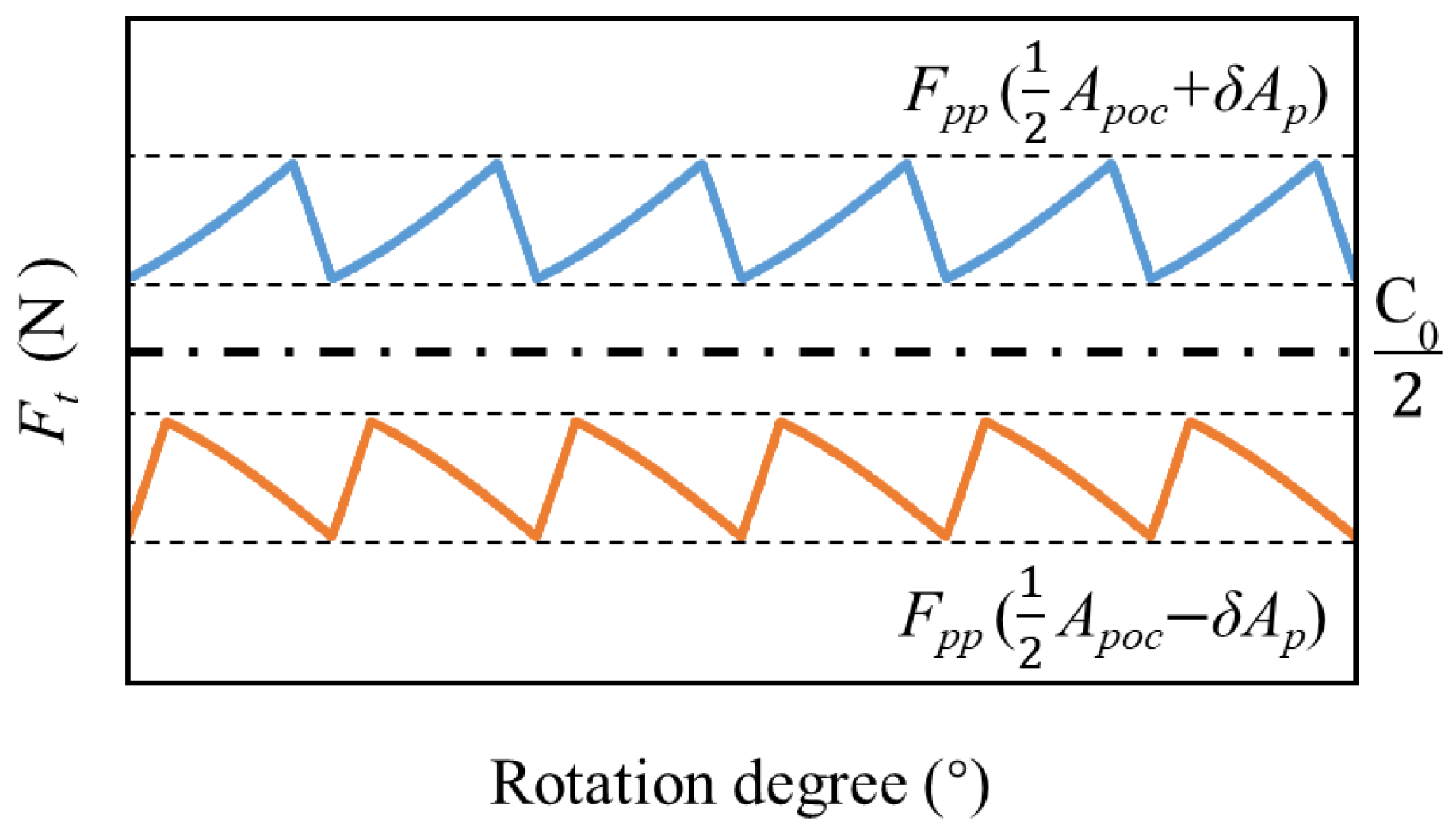
3.4. Symmetry Characteristics of Force Fluctuation

The characteristics of milling force fluctuations have been widely studied. It has been shown that the smaller the range of the study is, the better the research process will be. Equation (22) shows that the research range of the milling force fluctuation can be reduced from infinity to (0, A_poc). However, this range can still be further reduced if more features are discovered. As shown in Figure 6, if there exists δA_p such that whatever the δA_p value is, the value of F_pp(S + δA_p) is always equal to the value of F_pp(S − δA_p); then the milling force fluctuation can be regarded as a symmetry function and S is the input symmetry axis. To prove the theory of symmetry characteristics, A_poc is divided into two parts: A_p1 and (A_poc − A_p1), which can be expressed as follows:

$$F\left({\theta }_0,A_{poc}\right)=F\left({\theta }_0,A_{p1}\right)+F\left({\theta }_0,A_{poc}-A_{p1}\right)=C_0.$$

(23)

If $\delta A_p=A_{p1}-\frac{A_{poc}}{2}$, then $\{\begin{array}{c}{A}_{p1}=\frac{A_{poc}}{2}+\delta A_p\hfill \\ A_{poc}-A_{p1}=\frac{A_{poc}}{2}-\delta A_p\hfill \end{array}$.

By substituting the above into Equation (23), Equation (23) can be transformed into a symmetry formula as follows:

$$F\left({\theta }_0,A_{poc}\right)=F\left({\theta }_0,\frac{1}{2}{A}_{poc}+\delta A_p\right)+F\left({\theta }_0,\frac{1}{2}{A}_{poc}-\delta A_p\right)=C_0.$$

(24)

According to Equation (24), the milling force is symmetrical on the axial depth of cut A_poc/2 and the output symmetry axis is C₀/2. When Equation (24) is substituted into Equation (9), which is the definition of force fluctuations, it can be observed that the two symmetrical milling force fluctuations are the same, which is expressed in Equation (25).

$$F_{pp}\left(\frac{A_{poc}}{2}+\delta A_p\right)=F_{pp}\left(\frac{A_{poc}}{2}-\delta A_p\right).$$

(25)

Therefore, within a cutting depth of A_poc, the milling force fluctuations in the first half are the same as those in the second half, which further reduces the research range of the milling force from (0, A_poc) to (0, A_poc/2).

As shown in Figure 6 and expressed by Equation (25), the milling force fluctuation is a symmetrical function within the cutting depth of A_poc. If Equations (24) and (25) are combined with Equation (22), which expresses the periodicity characteristics of force fluctuation, the extended expression of the infinite symmetry axis S can be obtained as:

$$S=\frac{n{A}_{poc}}{2},\left(n=1,2,3\dots \right).$$

(26)

4. Simulation and Experimental Validation

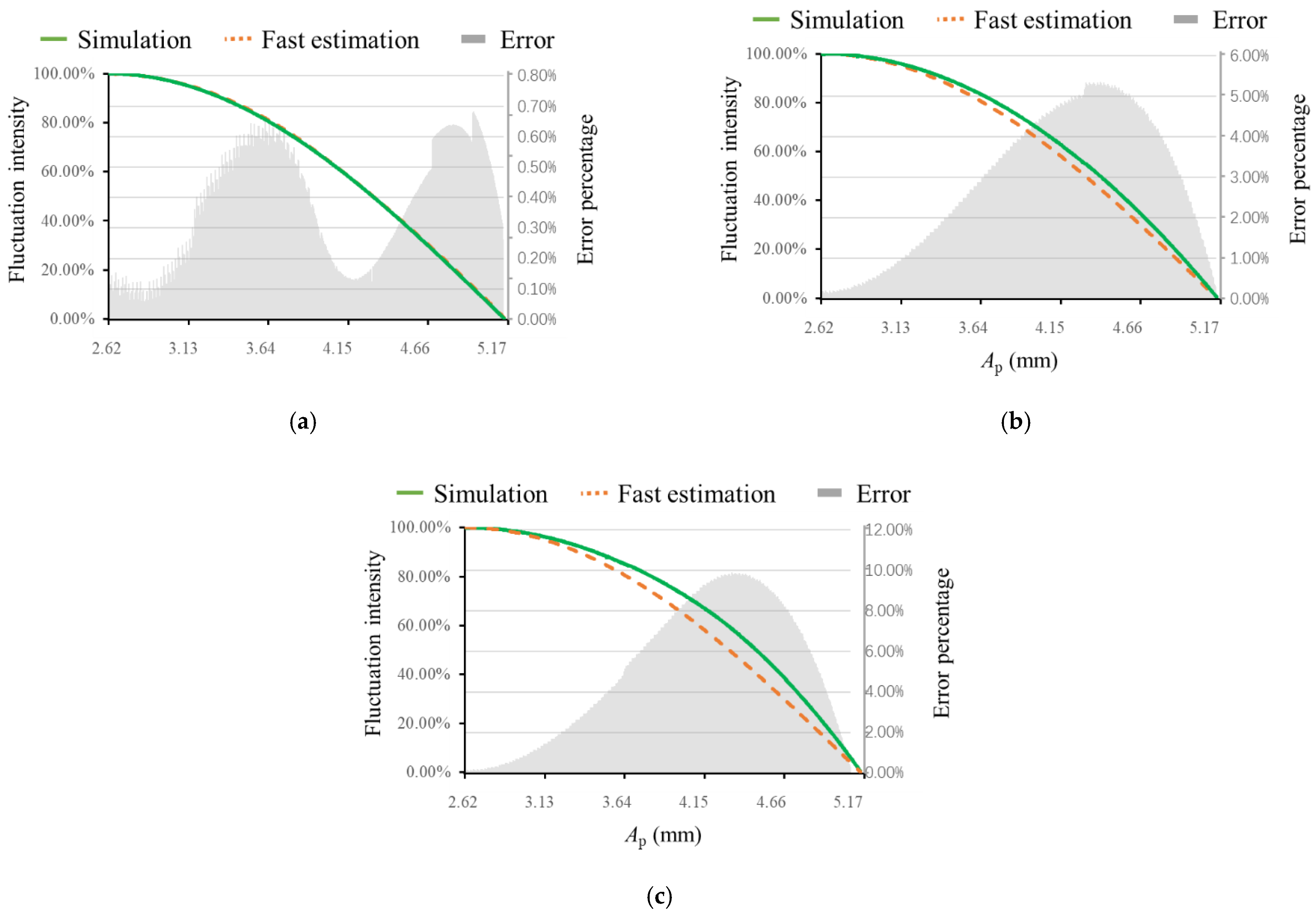
4.1. Fast Estimation Method of Milling Force Fluctuations

The characteristics of milling force fluctuations have been discussed in detail in the previous section, but the derived theory is a qualitative description. In order to quantify the intensity of force fluctuation, two prediction methods are proposed: fast estimation and accurate simulation. The fast estimation method introduces an intensity indicator related to the axial depth of cut to approximately estimate the force fluctuation.

Due to the periodicity and continuity characteristics, the fluctuation of the milling force must have minimum and maximum values in a period. Therefore, the intensity indicator of the milling force fluctuation can be expressed by a value varying from zero to 100%. Then, the symmetry characteristic makes the fluctuation of the first and second half periods symmetrical. Hence, milling force fluctuations in a period can be divided into two parts: the ascending part and the descending part. These two parts share the converse indicator. Therefore, the research range of A_p is reduced to [0, A_poc/2]. According to Equations (8) and (9), the milling force increases with the value of A_p when the engaged angle θ_en is bigger than (A_p × tan(β)/R). For fast estimation, assume that the relationship between A_p and F_pp are approximated to a sine function. Then, the intensity indicator (I_i) for fast estimation of the milling force fluctuation can be expressed as:

$$I_i=\left|sin\left(\frac{\pi A_p}{A_{poc}}\right)\right|\times 100\%,\left({\theta }_{en}\ge \frac{A_{p}tan\beta }{R}\right).$$

(27)

where,

$${\theta }_{en}=\{\begin{array}{cc}{\theta }_{ex}-{\theta }_{st}& ,down milling\\ {\theta }_{st}-{\theta }_{ex}& ,up milling\end{array}.$$

(28)

It should be noted that the intensity indicator is an approximate value for a fast estimate and it is affected by A_e, so it can be used to estimate the milling force fluctuation only with a low precision requirement.

4.2. Accurate Simulation Method of Milling Force Fluctuation

In order to predict the milling force fluctuations more accurately, a method for accurate simulation of the milling force fluctuations is proposed. The flowchart of this method is shown in Figure 7.

As shown in Figure 7, at the beginning of the simulation, before calculation, it is required to determine the milling parameters, including the milling cutter parameters and processing parameters. The cutter parameters include the number of helical edges, the cutter radius, helix angle and cutter rotation angle, and the processing parameters include the radial depth of cut, axial depth of cut, feed per tooth and force coefficients. Next, the milling type is determined according to these parameters. The entrance and exit angles of different milling types are calculated using Equations (4) and (5), respectively. Then, two parallel calculations are carried out to improve calculation efficiency. By using different initial angles, the force generated at each angle is calculated by Equation (8) and stored in a database. After that, the force fluctuation of one period is calculated by Equation (9). Further, by using different initial values of A_p, another parallel computation is performed to show the characteristics of force fluctuation at different axial depths of cut. Finally, the curves of force fluctuations and axial cutting depth are drawn based on the recorded data.

The error between the fast estimation model and the accurate simulation method is verified using the parameters given in

Table 1. Parameters for the force fluctuation simulation.

Processing Parameters	Value	Cutter Parameters	Value
ft	0.02 (mm/tooth)	Nt	6
Apoc	5.236 (mm)	β	45°
Ap	2.618–5.236 (mm)	R	5 (mm)
Ae	1.5, 2.5, 3.5 (mm)	Kt	474 (N/mm2)

. As mentioned below Equation (25), the research range of axial depth of cut is (0, A_poc/2). But the zero point of A_p cannot be verified in the simulation; the range of A_p is selected to be at the descending area of the first period, where the range of A_p is [A_poc/2, A_poc]. To measure the influence of the radial depth of cut, three A_e of 1.5, 2.5 and 3.5 mm were selected in the experiment. The comparison of the results of the two proposed methods are presented in Figure 8, where it can be seen that the error of the fast estimation method is related to A_e and A_p. At the values of A_e of 1.5, 2.5 and 3.5 mm, the maximum error of the fast estimation method has the values of 0.65%, 5.32% and 9.81%, respectively. Thus, the error is gradually increasing, which makes the fast estimation method more suitable for the smaller radial depth of cut. In addition, in Figure 8, the relationship between the error and A_p can be clearly observed. The smallest error is always at two points, A_poc and A_poc/2. As shown in Figure 8a, as the value of A_p moves away from the symmetry axis, the maximum error appears at A_p = 3.63 mm and A_p = 4.86 mm. However, different conclusions can be drawn based on the results presented in Figure 8b,c, where the fluctuation error has only one maximum value at A_p = 4.4 mm. The reasons for the inconsistency of results presented in Figure 8a–c can be the extremely small estimation error and unsatisfactory simulation accuracy. Finally, based on the three comparison results, it can be concluded that the overall error of the fast estimation method is not more than 10%. Therefore, if the value of A_e is small and the accuracy requirement is low, then the fast estimation method is suitable and effective. Otherwise, the simulation prediction method will be more appropriate.

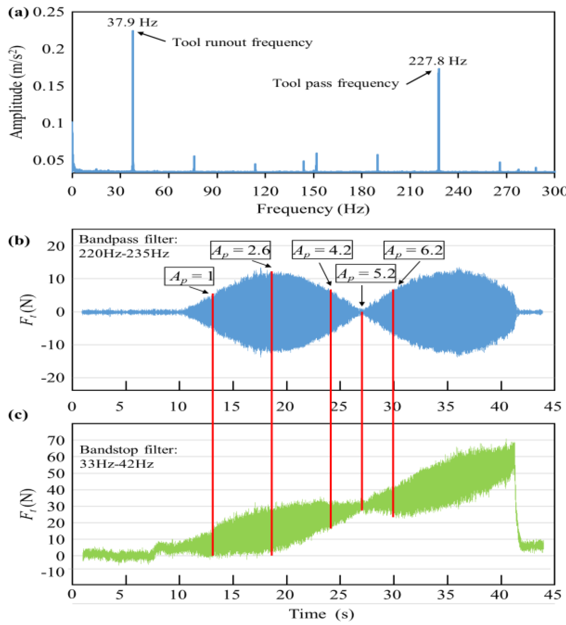
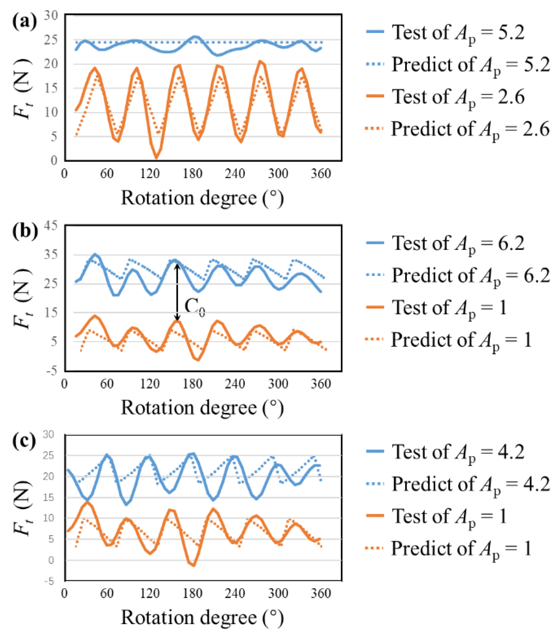
4.3. Experimental Validation of Force Fluctuation Characteristics

In this section, a milling experiment with a variable axial depth of cut is presented to verify the proposed theory of uniformity and periodicity and symmetry characteristics of force fluctuations. The milling experiment was conducted using the VMC-C50 machine tool (Shanghai TOP Numerical Control Technology Co., Ltd., Shanghai, China). The milling scheme is given in

Table 2. Milling scheme of the experiment.

Number	Ae (mm)	Ap (mm)	Feed Speed (mm/min)	Spindle Speed (rpm)
1	2.5	1	240	2279.8
2	2.5	2.618	240	2279.8
3	2.5	4.236	240	2279.8
4	2.5	5.236	240	2279.8
5	2.5	6.236	240	2279.8
6	2.5	0–10	240	2279.8

and the experimental parameters are given in

Table 3. Experimental conditions of the milling test.

Processing Parameters	Value	Cutter Parameters	Value
Milling type	Down milling	Nt	6
Cutting speed	71.6 (m/min)	β	45°
ft	0.017 (mm/tooth)	R	5 (mm)

. In order to make the experiment more accurate, the values of the spindle speed and K_t given in Table 2 were revised to an average of repeated measurements.

As shown in Figure 9a, the 9171A rotary dynamometer (Kistler, Winterthur, Switzerland) was used to collect the force fluctuation data of F_t and the sampling rate was 2 kHz. In order to avoid the noise from other signals, the dynamometer used a low-pass filter with a cut-off frequency of 300 Hz. The milling cutter had six helical-edges with an effective length of 40 mm, a radial rake angle of 8° and an axial rake angle of 12°. The workpiece was made of aluminum alloy (A5052), which was pre-processed into a shape of 200 × 10 × 50 mm. Its chemical composition is presented in

Table 4. Chemical composition and hardness of the A5052 aluminum alloy.

Chemical Composition (%)								Webster Hardness (HW)
Si	Fe	Cu	Mn	Mg	Cr	Zn	Al
<0.25	<0.4	<0.1	<0.1	2.2–2.8	0.15–0.35	<0.1	remain	11

. The milling process was side milling and the other parameters used in the experiments are similar to the parameters in Section 4.2.

In particular, the change in the axial position of the milling cutter presented in Figure 9b is demonstrated only for the purpose of easier understanding. During the milling experiment, the milling cutter was fixed at the position of 10 mm and the change in the value of A_p was caused by the shape of the workpiece, which was an oblique triangle shape and gradually became higher during milling process. Then, the five marking points of A_p = 1 mm, A_p = 2.6 mm, A_p = 4.2 mm, A_p = 5.2 mm and A_p = 6.2 mm were used to verify the theory of milling force fluctuation characteristics.

The force fluctuations of the fast estimation method and the process of the milling experiment are presented in Figure 9b. As mentioned in Section 4.1, the cutting area varies with the axial depth of cut from zero to 10 mm, containing two periods, where each period is composed of the ascending and descending parts. The milling force fluctuates to the maximum on the symmetry axis and fluctuates to the minimum on the periodic axis. Then, a comparative experiment between the fast estimation method and the test force data was performed.

The corresponding experimental data are shown in Figure 10. The frequency of the milling force was analyzed by the FFT method. As shown in Figure 10a, there are two main frequency bands, one is the tooth passing frequency at 227.8 Hz and the other is the tool runout frequency at 37.9 Hz. The difference between two frequency is 6 times, which is exactly equal to the number of cutting edges [25]. For the purpose of the obvious display of force fluctuations generated by each cutting edge, the force fluctuation data at tool pass frequency were extracted by a band-pass filter with a frequency range of 220 Hz to 235 Hz and the force results are shown in Figure 10b. The experimental results were consistent with those of the fast estimation method. The maximum fluctuation of the milling force was 23.12 N and it was observed at two positions on the symmetry axis, at A_p = 2.62 mm and A_p = 7.85 mm; meanwhile, the minimum fluctuation was 1.08 N and it was observed at the position of A_p = 5.23 mm on the period axis. Due to the accuracy of the experiment, it is acceptable that the minimum value is not zero. Both the fast estimation results of Figure 10a and the experimental results of Figure 10b show the proposed force fluctuation characteristics. Furthermore, the experimental results in Figure 10b show that the force fluctuation characteristics with the axial depth of cut from zero to 10 mm can be expressed by the part with the axial depth of cut from zero to 2.6 mm. Therefore, the experimental result also verified that 75% of the experimental workload in Figure 9b can be reduced. By applying the proposed force fluctuation theory, the milling force fluctuations of all depths of cut can be represented by the milling force fluctuation characteristics of the first half period (A_poc/2). Then, as the research range of A_p increases, more testing workload can be saved.

When the axis position of the force fluctuation on the force curve was determined in Figure 10b, the positions of the marking points in the force curve were determined based on the time interval and axis position. The values of A_p = 1 mm, A_p = 2.6 mm, A_p = 4.2 mm, A_p = 5.2 mm and A_p = 6.2 mm on the curve corresponded to the times of 13.2, 18.7, 24.1, 27.4 and 30.6 s, respectively. With the use of the same time label, the marked points were projected onto the force fluctuation data of the milling experiment, as shown in Figure 10c.

The milling force in Figure 10c was used to determine the difference between the simulation method and the experimental test. The results showed that the average error of the simulation method was less than 3 N and this method was more accurate than the fast estimation method. In order to reduce the force fluctuation caused by the cutter runout, the collected data were filtered with a band-pass filter of a cutter runout frequency of 33 to 42 Hz. The milling force near the marked points was extracted and the obtained results of uniformity, periodicity and symmetry characteristics of force fluctuations are displayed in Figure 11a–c respectively.

The results presented in Figure 11a verify the uniformity characteristics of the milling force fluctuation theory. The minimum value of the milling force fluctuation with A_poc, which was calculated by Equation (14), was compared with the actual measured milling force fluctuation. The tested amplitude of the milling force fluctuation was 24.5 N with a slight fluctuation of 3 N, which could be caused by the influence of filtering and other noise data. The measured milling force at A_p = 2.6 mm was used for comparison of the simulation error. The comparison of the two force fluctuations showed that the simulation method could accurately predict the milling force fluctuations with an error of less than 3 N. This comparison also confirmed by the correctness of the uniformity characteristics of the milling force fluctuations.

The results presented in Figure 11a verify the uniformity characteristics of the milling force fluctuation theory. The minimum value of the milling force fluctuation with A_poc, which was calculated by Equation (14), was compared with the actual measured milling force fluctuation. The tested amplitude of the milling force fluctuation was 24.5 N with a slight fluctuation of ±1.5 N, which could be caused by the influence of filtering and other noise data. The measured milling force at A_p = 2.6 mm was used for comparison of the simulation error. The comparison of the two force fluctuations showed that the simulation method could accurately predict the milling force fluctuations with an error of less than 3 N. This comparison also confirmed the correctness of the uniformity characteristics of milling force fluctuations.

The results in Figure 11b verify the periodicity characteristics of the milling force fluctuation theory. Although there were certain differences between the measured and simulation data, due to the simplified force prediction model, the measured data at A_p = 1 mm are high similarity with the measured data at A_p = 6.2 mm, having a constant difference of approximately 23N. This result proves the correctness of the periodicity theory defined by Equation (22).

The results in Figure 11c show two sets of force data at A_p = 1 mm and A_p = 4.2 mm; the first A_p is arbitrary and the second one is determined according to Equation (25). The collected data were realigned by the fluctuation characteristics of the milling force. As shown in Figure 11c, the force fluctuation at A_p = 1 mm was approximately 9.5 N and that at A_p = 4.2 mm was approximately 8 N. Due to the instability of milling force fluctuations, a small, inconsistent fluctuation of 1.5 N can be regarded as a calculation error. Therefore, Equation (23) is verified to be correct. Then, other features of the symmetry characteristics of Equations (24) and (26) can also be observed in Figure 11c. Based on the comparison results of the two sets of data, it can be concluded that the two forces were symmetrical on the input axis of A_p = 2.6 mm and the output axis of F = 12.5 N. This result confirmed the proposed symmetry characteristics of the milling force fluctuation theory.

5. Conclusions

This study presents three characteristics of milling force fluctuations: uniformity, periodicity and symmetry. By applying the proposed theory, it is only needed to test the force fluctuations in the range of [0, A_poc/2] to obtain the actual force fluctuations in the range of [0, +∞]. This greatly reduces the test workload of a milling force experiment on the axial depth of cut and makes the proposed theory a useful approach during the study and development of a new advanced milling process.

The main contributions of this study can be summarized as follows:

• A milling force modeling method is proposed to fulfill the requirements of mathematical expression of the milling force fluctuation. By using the peak-to-peak difference of milling force, the milling force fluctuations are quantified and defined, which provides an opportunity to study the characteristics of milling force fluctuations by mathematical methods;
• A virtual-edge projection method, which enables the milling force on every cutting edge to be projected and replaced directly to the same virtual edge, is proposed. Therefore, the milling force fluctuation can be analyzed intuitively from discontinuities and overlaps of the projected virtual edge;
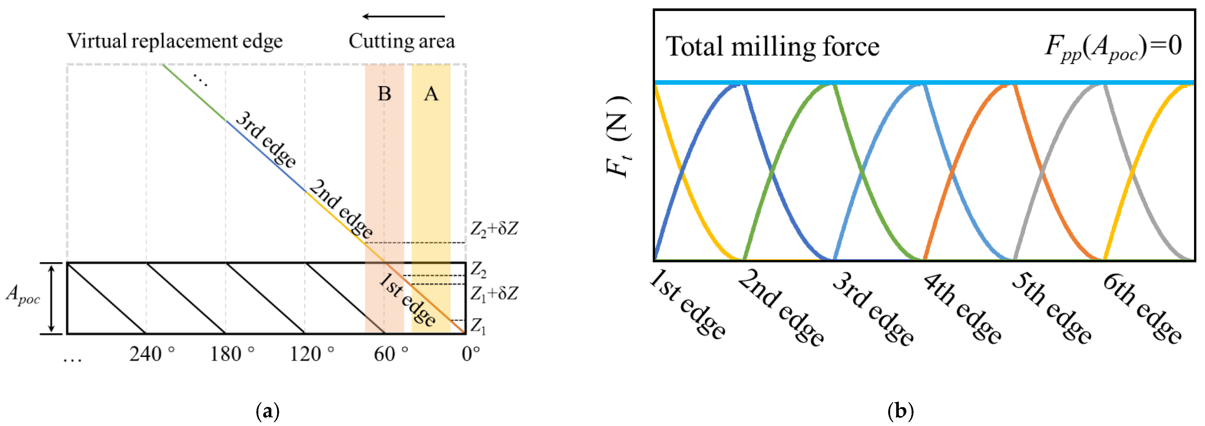
• The relationship between the force fluctuation characteristics and axial depth of cut is revealed. A one-cycle standard of the axial depth of cut (A_poc) is defined. It is also proven that the force fluctuation is always zero when the axial depth of cut is A_poc. In addition, it is demonstrated that the milling force fluctuates periodically and the minimum period is A_poc. Furthermore, in a period, the milling force fluctuation always first ascends and then descends as the value of A_p increases and the amplitude is symmetric about A_poc. Then, the milling force fluctuations of all periods can be understood by experimental test of only half periods, which significantly reduced the milling test workload;
• Two prediction methods of milling force fluctuations are proposed: fast estimation method and simulation method. The fast estimation method has a simple calculation process and does not require determining the milling force coefficient. However, it only displays a percentage result of force fluctuations and there is no specific force value, which makes this method less accurate and suitable for precise engineering applications. In contrast, the simulation method has higher prediction accuracy and the average error is less than 3 N, which meets the experimental requirements.

In summary, this study reveals the force fluctuation characteristics in different axial depths of milling and proposes the theory of uniformity, periodicity and symmetry. The application of this theory can not only reduce the test workload, but also predict and understand the actual force fluctuations at different axial depths of milling. In future work, we will study the relationship between milling force fluctuation characteristics and other parameters, such as radial depth of cut.

References

1. Xu, D.; Liao, Z.; Axinte, D.; Hardy, M. A novel method to continuously map the surface integrity and cutting mechanism transition in various cutting conditions. Int. J. Mach. Tools Manuf. 2020, 151, 103529. [Google Scholar] [CrossRef]
2. Li, H.; Zeng, H.; Chen, X. An experimental study of tool wear and cutting force variation in the end milling of Inconel 718 with coated carbide inserts. J. Mater. Process. Technol. 2006, 180, 296–304. [Google Scholar] [CrossRef]
3. Desai, K.A.; Rao, P.V.M. On cutter deflection surface errors in peripheral milling. J. Mater. Proc. Tech. 2012, 212, 2443–2454. [Google Scholar] [CrossRef]
4. Pimenov, D.Y.; Hassui, A.; Wojciechowski, S.; Mia, M.; Gupta, M.K. Effect of the relative position of the face milling tool towards the workpiece on machined surface roughness and milling dynamics. Appl Sci. 2019, 9, 842. [Google Scholar] [CrossRef] [Green Version]
5. Leal-Muñoza, E.; Diezb, E.; Perezc, H.; Vizan, A. Accuracy of a new online method for measuring machining parameters in milling. Measurement 2018, 128, 170–179. [Google Scholar] [CrossRef]
6. Erkorkmaz, K.; Altintas, Y. Quintic Spline Interpolation with Minimal Feed Fluctuation. J. Manuf. Sci. Eng. 2005, 127, 339–349. [Google Scholar] [CrossRef]
7. Wang, Q.H.; Liao, Z.Y.; Zheng, Y.X.; Li, J.-R.; Zhou, X.-F. Removal of critical regions by radius-varying trochoidal milling with constant cut-ting forces. Int. J. Adv. Manuf. Technol. 2018, 98, 671–685. [Google Scholar] [CrossRef]
8. Ma, J.-W.; Song, D.-N.; Jia, Z.-Y.; Hu, G.-Q.; Su, W.-W.; Si, L.-K. Tool-path planning with constraint of cutting force fluctuation for curved surface machining. Precis. Eng. 2018, 51, 614–624. [Google Scholar] [CrossRef]
9. Altinta, Y.; Lee, P. A General Mechanics and Dynamics Model for Helical End Mills. Ann. CIRP 1996, 45, 59–64. [Google Scholar] [CrossRef]
10. Budak, E.; Altintaş, Y.; Armarego, E.J.A. Prediction of Milling Force Coefficients from Orthogonal Cutting Data. J. Manuf. Sci. Eng. 1996, 118, 216–224. [Google Scholar] [CrossRef]
11. Engin, S.; Altintas, Y. Mechanics and dynamics of general milling cutters—Part I: Helical end mills. Int. J. Mach. Tools Manuf. 2001, 41, 2195–2212. [Google Scholar] [CrossRef]
12. Li, H.Z.; Liu, K.; Li, X.P. A new method for determining the undeformed chip thickness in milling. J. Mater. Proc. Tech. 2001, 113, 378–384. [Google Scholar] [CrossRef]
13. Wojciechowski, S.; Matuszak, M.; Powałka, B.; Madajewski, M.; Maruda, R.W.; Królczyk, G.M. Prediction of cutting forces during micro end milling considering chip thickness accumulation. Int. J. Mach. Tools Manuf. 2019, 147, 103466. [Google Scholar] [CrossRef]
14. Desai, K.A.; Piyush, K.A.; Rao, P.V.M. Process geometry modeling with cutter runout for milling of curved surfaces. Int. J. Mach. Tools Manuf. 2009, 49, 1015–1028. [Google Scholar] [CrossRef]
15. Lin, B.; Wang, L.; Guo, Y. Modeling of cutting forces in end milling based on oblique cutting analysis. Int. J. Adv. Manuf. Technol. 2016, 84, 727–736. [Google Scholar] [CrossRef]
16. Schwenzer, M.; Auerbach, T.; Dbbeler, B.; Bergs, T. Comparative study on optimization algorithms for online identification of an instantaneous force model in milling. Int. J. Adv. Manuf. Technol. 2019, 101, 2249–2257. [Google Scholar] [CrossRef]
17. Gowthaman, S.; Jagadeesha, T. Influence of radial rake angle and cutting conditions on friction during end milling of Ni-monic 263. Int. J. Adv. Manuf. Technol. 2020, 109, 247–260. [Google Scholar] [CrossRef]
18. Ghani, J.A.; Choudhury, I.A.; Hassan, H.H. Application of Taguchi method in the optimization of end milling parameters. J. Mater. Proc. Technol. 2004, 145, 84–92. [Google Scholar] [CrossRef]
19. Jiang, F.; Zhang, T.; Yan, L. Analytical model of milling forces based on time-variant sculptured shear surface. Int. J. Mech. Sci. 2016, 115–116, 190–201. [Google Scholar] [CrossRef]
20. Sahoo, P.; Patra, K.; Singh, V.K.; Gupta, M.; Pimenov, D.Y. Influences of TiALN coating and limiting angles of flutes on prediction of cutting forces and dynamic stability in micro milling of die steel (P-20). J. Mater. Proc. Technol. 2020, 278, 116500. [Google Scholar] [CrossRef]
21. Liu, X.-W.; Cheng, K.; Webb, D.; Lou, X.-C. Prediction of cutting force distribution and its influence on dimensional accuracy in peripheral milling. Int. J. Mach. Tools Manuf. 2002, 42, 791–800. [Google Scholar] [CrossRef]
22. Yang, L.; Devor, R.E.; Kapoor, S.G. Analysis of Force Shape Characteristics and Detection of Depth-of-Cut Variations in End Milling. J. Manuf. Sci. Eng. 2004, 127, 454–462. [Google Scholar] [CrossRef]
23. Arshinov, V.A.; Alekseev, G.A. Metal Cutting Theory and Cutting Tool Design; Mir Publishers: Moscow, Russia, 1976. [Google Scholar]
24. Huang, W.; Li, X.; Wang, B.; Chen, J.; Zhou, J. An analytical index relating cutting force to axial depth of cut for cylindrical end mills. Int. J. Mach. Tools Manuf. 2016, 111, 63–67. [Google Scholar] [CrossRef]
25. Liang, S.Y.; Wang, J.J.J. Milling force convolution modeling for identification of cutter axis offset. Int. J. Mach. Tools Manuf. 1994, 34, 1177–1190. [Google Scholar] [CrossRef]
Figure 1. Milling geometry and mechanism of a helical-edge cutter: (a) process of down milling and (b) the distribution of milling forces.
Applsci 11 02693 g001
Figure 2. Expansion of the cutter-workpiece engagement.
Applsci 11 02693 g002
Figure 3. Transformation of the milling force: (a) milling at different positions with equal axial cutting depth and (b) the virtual-edge projection.
Applsci 11 02693 g003
Figure 4. The uniformity characteristics of force fluctuation: (a) virtual-edge projection and (b) the force fluctuation of uniformity milling.
Applsci 11 02693 g004
Figure 5. The periodicity characteristics of force fluctuation.
Applsci 11 02693 g005
Figure 6. The symmetry characteristics of force fluctuation.
Applsci 11 02693 g006
Figure 7. Simulation process of force fluctuation.
Applsci 11 02693 g007
Figure 8. Comparison of the fast estimation method and the simulation method: (a) Ae = 1.5 mm; (b) Ae = 2.5 mm; and (c) Ae = 3.5 mm.
Applsci 11 02693 g008
Figure 9. Experimental validation of the force fluctuation characteristics: (a) experimental environment and (b) description of the milling process and the fast estimation method.
Applsci 11 02693 g009
Figure 10. Experiment result and force fluctuation data: (a) FFT analysis at spindle speed 2279.8 rpm, Ae = 2.5 mm, Ap = 0~10 mm; (b) milling force fluctuation data at tool pass frequency and (c) milling force data without cutter runout influence.
Applsci 11 02693 g010
Figure 11. Enlarged view of milling force data: (a) enlarged view of the milling force data at Ap = 2.6 mm and Ap = 5.2 mm; (b) enlarged view of milling force data at Ap = 1 mm and Ap = 6.2 mm; and (c) enlarged view of the milling force data at Ap = 1 mm and Ap = 4.2 mm.
Applsci 11 02693 g011