Article

3D Cavitation Shedding Dynamics: Cavitation Flow-Fluid Vortex Formation Interaction in a Hydrodynamic Torque Converter

School of Mechanical and Aerospace Engineering, Jilin University, Changchun 130022, China
*
Author to whom correspondence should be addressed.
Appl. Sci. 2021, 11(6), 2798; https://doi.org/10.3390/app11062798
Submission received: 5 February 2021 / Revised: 17 March 2021 / Accepted: 19 March 2021 / Published: 21 March 2021
(This article belongs to the Special Issue Turbomachinery: Theory, Design and Application)

Abstract

:
Recent experiments have shown interactions between the cavitation and fluid vortex formation in a hydrodynamic torque converter. This study aimed to clarify the unsteady cavitation trigger mechanism and flow-induced vibration caused by turbulence–cavitation interactions. The mass transfer cavitation model and modified Reynolds-averaged Navier–Stokes k–ω model were used with a local density correction for turbulent eddy viscosity to investigate the cavitation structure in a hydrodynamic torque converter under various operating conditions. The model results were then validated against test data. The multi-block structured gridding technique was used to develop an orthogonally structured grid of a three-dimensional full-flow passage as an alternative analysis method for the cavitation flow. The results indicated that the re-entrant jet is the main cause of the shedding cavitation and breaking O-type cavitation. The re-entrant jet is driven by the reverse pressure gradient to move upstream towards the stator nose, and it lifts and splits the attached cavitation, which periodically induces shedding cavitation. When the cavitation was considered, the prediction error of the capacity constant was reduced from 13.23% to <5%. This work provides an insight into the cavitation–vortex interactions in a hydrodynamic torque converter, which can be used to improve the prediction accuracy of the hydrodynamic performance.

1. Introduction

The hydrodynamic torque converter is a typical coupled turbomachine that transfers power via the interaction between the blades and transmission medium. A hydrodynamic torque converter can provide a high output torque at a speed ratio (SR) of zero. Thus, the working machine has good launching performance and the advantages of fluid coupling and vibration damping. A hydrodynamic torque converter typically comprises three elements: a turbine driving the transmission, a pump driven by an engine, and a stator mounted on an overrunning clutch between the pump and turbine [1,2,3].
In recent years, hydrodynamic torque converters have been designed with increased launching performance, power density, and rotation speed, which can increase the risk of cavitation. Cavitation reduces the performance of a hydrodynamic torque converter, and its inception and development destabilize the rotation speed. Cavitation has been observed in many types of turbomachines, as shown in Figure 1. Bakir studied the relationship between the head drop of the inducer and cavitation under the different flow rates conditions. They found that under a specific range of the flow rate, the computational fluid dynamics (CFD) results agreed well with the test [4]. Brennen studied the cavitation behavior inside a scaled pump. A large number of cavitation bubbles at the trailing edge of the pump were observed in their research [5]. Park tested the fully developed cavitation form of the propeller. The sheet cavitation and tip vortex cavitation were found in their study [6]. Tsutsumi employed a transparent torque converter model to observe the cavitation form and location at low rotational speeds. A large number of attached cavitation were found at the leading edge of the stator [7]. Other researchers have studied cavitation in axial flow pump, water pump, etc. [8,9,10]. Most of their research focuses on experimental observation and performance testing, but only a few reports are available on the cavitation mechanism and transient cavitation behavior of hydrodynamic torque converters.
Microwave telemetry, nearfield acoustic measurement, and particle image velocimetry can be employed to predict the cavitation formation and process in a hydrodynamic torque converter [11,12,13,14,15,16,17]. Nearfield acoustic measurement has been employed to directly detect the cavitation effect of the flow field in a hydrodynamic torque converter with different blade geometries [18,19,20]. Watanabe et al. performed numerical simulations to predict the cavitation behavior of a hydrodynamic torque converter at SR = 0 and established a relationship between cavitation and vibration [21]. Ju et al. studied the relationship between the cavitation and performance of a hydrodynamic torque converter. They reported that cavitation occurs mainly near the stator nose when SR = 0. Cavitation can cause the stall capacity constant (CC0) and stall torque ratio (TR0) to drop drastically with advanced flow separation near the stator [22]. Liu et al. proposed removing the interface between the turbine and stator when simulating the cavitation of a hydrodynamic torque converter and setting a reference pressure level at the pump–stator interface near the shell, which can increase the convergence and accuracy of a two-phase flow cavitation simulation [23]. Previous research mainly employed a periodic steady-state single-flow passage or a series of experimental tests to predict the cavitation flow field of a hydrodynamic torque converter. However, the strong interaction between the blades and flow field means that the cavitation in a hydrodynamic torque converter cannot be in a stable state, and the cavitation bubbles must exhibit dynamic behavior. The relationship between this dynamic behavior and torque is not well recognized. The evolution mechanism and flow-induced vibration of transient cavitation inside the hydrodynamic torque converter still need to be clarified.
This study focused on the evolution of transient cavitation in the torque converter and the flow-induced vibration caused by cavitation–turbulence interaction. The aim was to clarify the cavitation mechanism of the flow field in a torque converter under the influence of a complex multiphase flow. The findings of this study may help in developing an effective cavitation suppression method for a turbomachine user.

2. Methodology

Because it is a transfer mechanism between the vapor and liquid phases, cavitation poses great challenges to the grid resolution and stability of numerical simulations. To simulate the transient cavitation phenomenon inside a hydrodynamic torque converter accurately, the Reynolds-averaged Navier–Stokes (RANS) with shear stress transport (SST) k–ω turbulence model and the Zwart–Gerber–Belamri cavitation model were employed to simulate the internal flow field of a hydrodynamic torque converter.

2.1. Turbulence Model

The turbulent flow field of the hydrodynamic torque converter was solved with RANS equations. The flow field of a hydrodynamic torque converter is considered as a mixture of vapor and liquid. The fluid in the flow field always maintains the conservation of mass and momentum, which can be expressed by the following equations.
Continuity equation:
ρ t + ( ρ u j ) x j = 0 .
Momentum equation:
( ρ u i ) t + ( ρ u i u j ) x j = ρ f i p x i + x j [ ( μ + μ t ) ( u i x j + u j x i 2 3 u k x k δ i j ) ] .
Mixture density:
ρ = α v ρ v + ( 1 α v ρ l ) .
In Equations (1) and (2), x i , u i , and f i are the components of the displacement, velocity, and body force, respectively, that are in the i direction. μ and μ t are the laminar and turbulent viscosities, respectively.
The governing equations in the SST k–ω model are for the turbulence kinetic energy k and specific dissipation rate ω:
( ρ k ) t + ( ρ k u i ) x i = x i [ ( μ + σ k μ t ) k x i ] + P k β * ρ k ω
( ρ ω ) t + ( ρ ω u i ) x i = x i [ ( μ + σ ω μ t ) ω x i ] β ρ ω 2 + 2 ( 1 F 1 ) ρ σ w 2 1 ω k x i ω x i + α ρ S 2
The blending function F1 is defined as
{ F 1 = tan h { { min [ m a x ( k β * ω y , 500 ν y 2 ω ) , 4 ρ σ ω 2 k C D k ω y 2 ] } 4 } C D k ω = m a x ( 2 ρ σ ω 2 1 ω k x i ω x i , 10 10 ) .
At the boundary layer, the kε model is employed away from the wall. When F1 = 0, the inner layer switches to the kω model. The turbulent viscosity is defined by
μ t = a 1 k m a x ( a 1 ω , S F 2 ) .
where S is the invariant measure of the strain rate. The second blending function F2 is defined as
F 2 = t a n h [ [ m a x ( 2 k β * ω y , 500 ν y 2 ω ) ] 2 ] .
In the stagnation zone, the SST k–ω turbulence model defines a production limiter to prevent turbulence generation, which is defined as
P k = μ t u i x j ( u i x j + u j x i ) .
Table 1 presents all constants in the SST k–ω turbulence model.

2.2. Cavitation Model

The mass transfer mechanism between the vapor and liquid phases is described using the Zwart–Gerber–Belamri cavitation model. The difference between the local and vapor pressures in the flow field drives the mass transfer rate between the vapor and liquid phases (i.e., the rate of cavitation in the flow field). The cavitating flow field is determined by the mass transfer rate between the vapor and liquid phase [24]. The cavitation rate is governed by the transport equation:
t ( α l ρ v ) + · ( α l ρ v V v ) = R e R c ,
where α l is the volume fraction of liquid phase, ρ v is the density of the vapor phase, V v is the velocity of the vapor phase, and R e and R c are the mass transfer source terms related to the evaporation and condensation, respectively, of the vapor.
The evaporation mechanism responsible for cavitation in the hydrodynamic torque converter flow field is governed by R e . When the local pressure in the flow field is less than the vapor pressure, the liquid phase partially converts to the vapor phase, which determines the formation of cavitation in the flow field. The source terms in Equation (10) for the evaporation are expressed by
R e = F vap 3 α nuc ( 1 α v ) ρ ν R B 2 3 p ν p ρ l .
The cavitation bubbles inside the hydrodynamic torque converter compress when they move toward the high-pressure region, and the cavitation condensation mechanism is determined by R c . When the local pressure in the flow field exceeds the vapor pressure, the vapor phase starts to condense. The source terms in Equation (10) for the condensation are expressed as
R c = F cond 3 α v ρ ν R B 2 3 p p ν ρ l ,
where p is the mixture pressure, p v is the vapor pressure, and ρ l is the density of liquid phase. Different empirical factors are assumed in ANSYS Fluent help profiles as follows: R B = 10−6 m, α nuc = 0.0005, F vap = 50, and F cond = 0.01.
The turbulence level of the flow is clearly related to the cavitation, and fluctuations in the turbulence velocity are greatly influenced by cavitation shedding. Therefore, the cavitation and turbulence models need to be combined to resolve the multiphase problem of the hydrodynamic torque converter, which is usually solved as a flow of pure oil with large prediction errors.

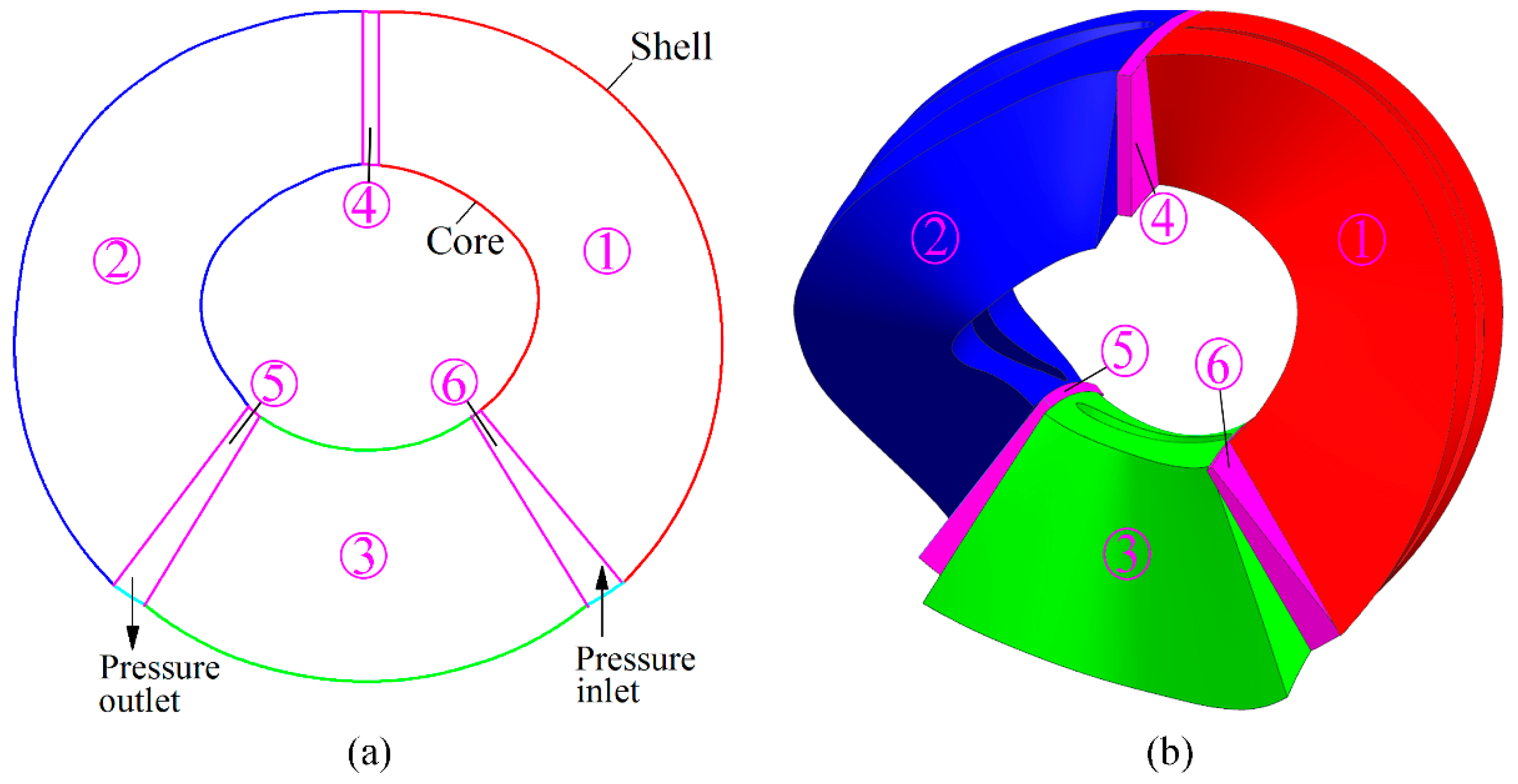
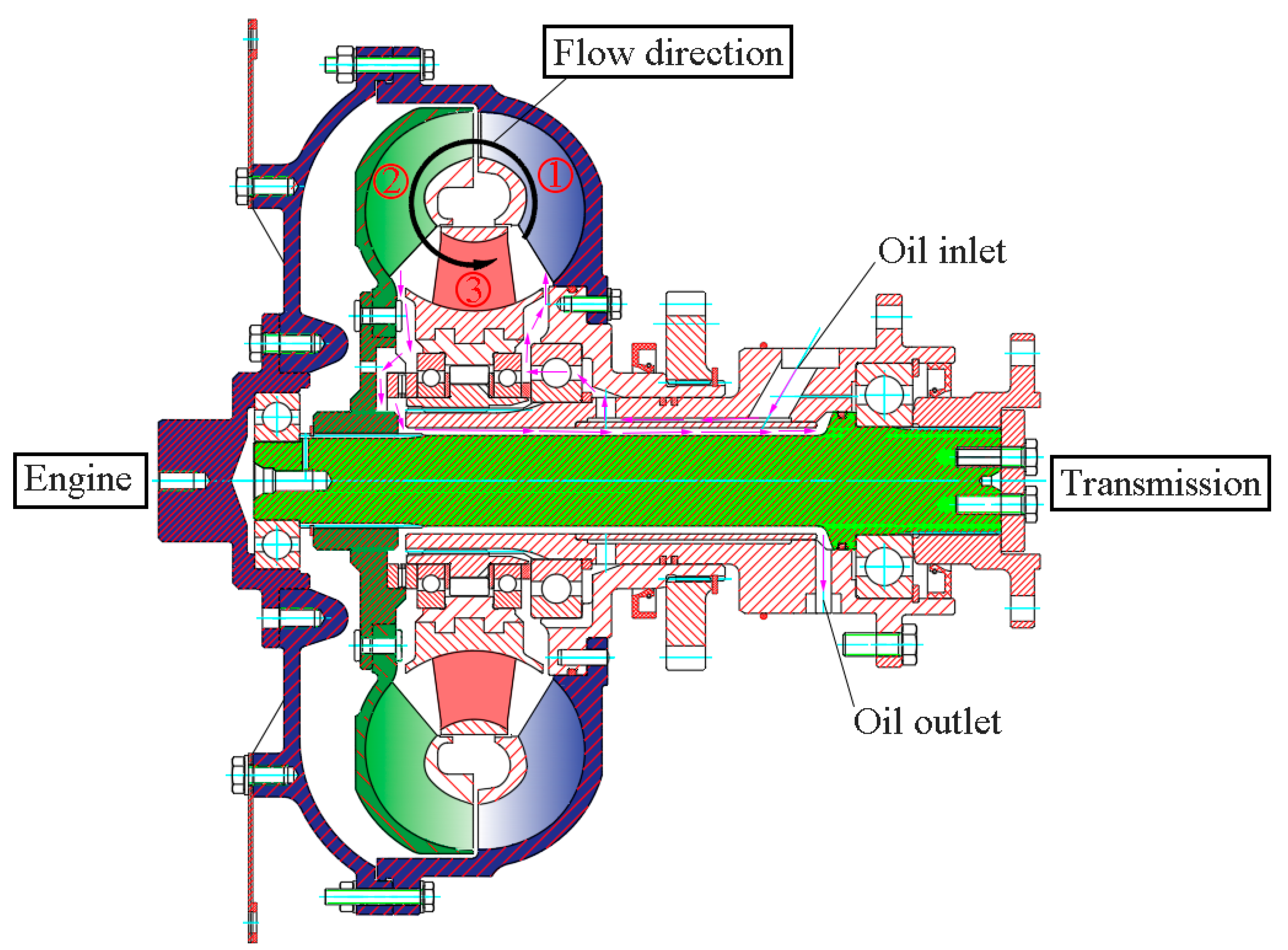
2.3. Simulation Setup

Many researchers employed the single flow passage to develop the cavitation flow field of the torque converter, and the internal flow field was always in highly developed transient turbulence. The rotor–stator interaction and turbulence between the impellers make the flow field distribution of a single flow passage no longer have rotational symmetrical characteristics. Obviously, the CFD model establishment is incorrect. The torus meridian view and the single flow passage are shown in Figure 2, which indicates the layout of the six domains of the torque converter in this paper. Except for pressure inlet (charge pressure, Figure 2a is displayed with a cyan line), pressure outlet (backpressure, Figure 2a is displayed with a cyan line), adjacent domains are connected by an interface, and the remaining boundaries are walls. Figure 3 is a cross-sectional view of the torque converter. According to the sectional view of the torque converter, the full-flow transient passage model was implemented in our study to increase the prediction accuracy for the hydrodynamic torque converter. The charge pressure and backpressure were set at 0.8 and 0.4 MPa, respectively, for the S–P and T–S clearances near the shell (Figure 4).
To capture the flow behavior around the blade, the grid element size near the blade was refined with 12 layers of prism elements. The grid element growth rate from the first layer to the following layer in the 12 layers of prism elements domain was 1.2, and the near-wall grid element height was 1 mm. To ensure that the average y+ value was <1, the height of the first layer grid element was set to 0.025 mm. Figure 4 was generated with the software ANSYS ICEM. To balance the relationship between computational effort and accuracy, a mesh independence study was performed. The simulation calculations of torque converter models with different grid densities were carried out under stall operating condition. Setting the same boundary conditions, algorithms, and convergence criteria, the CFD results under different grid elements are shown in Figure 5. The results indicated that refining the grid had a small effect on the torque when the global grid element size was 3 mm. The commercial software ANSYS FLUENT was used to simulate CFD models comprising 4.48 × 10⁶ grid elements with a global grid element size of 3 mm.
Compared with single-phase simulation, converging a multiphase simulation is very challenging. To improve the convergence and accuracy, the time step of the multiphase-flow simulation was reduced five times compared with that of the single-phase flow simulation. The Zwart–Gerber–Belamri cavitation model was employed, which is more stable than that of Singhal et al. cavitation model [25]. The time step was taken as 0.0001 s. In total, 1200 time steps were calculated, during which time, the pump completed at least four revolutions. Table 2 presents the details of the CFD model parameters.

3. Transient Cavitation Behavior in a Hydrodynamic Torque Converter

3.1. Validation of the CFD Model

The detailed specifications of the pump, turbine, and stator are summarized in Table 3.
The hydrodynamic performance of a torque converter is defined by several operating parameters that are described as follows.
S R   ( Speed   ratio ) :   S R = T Turbine N Pump
T R ( T o r q u e   r a t i o ) : T R = T Turbine T Pump
η   ( Efficiency ) :   η = N Turbine × T Turbine N Pump × T Pump = S R × T R
C C   ( Capacity   constant ) :   C C = T Pump ρ g N Pump 2 D 5 ,
where N Pump and T Turbine are the rotational speed (rpm) and T Pump and T Turbine are the torque (N m) of pump and turbine, respectively. D represents the diameter of the torus.
CC represents the capacity of the power transmission, 10−6 min 2 r 2 m 1 .
The details of the hydrodynamic performance calculation and experimental apparatus of the hydrodynamic torque converter were reported previously [26]. CFD models with and without cavitation were used. Figure 6 compares the calculated hydrodynamic performances with the test data. The calculated hydrodynamic performances were consistent at high SRs (SR ≥ 0.3). However, the CFD models differed tremendously in terms of the torque ratio and capacity constant at low SRs (SR < 0.3). The experimental data indicated that the capacity constant increased with increasing SR at low SRs, whereas the trend reversed at high SRs. The calculated capacity constant without cavitation did not show this trend with a maximum error of 13.23% under the stall operating condition. In contrast, the calculated capacity constant with cavitation had a maximum error of <5% at low SRs. The capacity constant considering cavitation increased with the SR, which agrees with the test data. The two CFD models returned slightly higher values than the test data at high SRs, which could be attributed to the flow leakage at the shell and core of the hydrodynamic torque converter being neglected. When SR ≥ 0.3, the two CFD models were consistent regarding the torque ratio. When SR < 0.3, the CFD models had maximum errors of 4% and 8% with and without cavitation, respectively, for the torque ratio.
The CFD results indicate that the development of cavitation reduces both TR and CC at low SRs (SR < 0.3). At high SRs (SR ≥ 0.3), the two CFD models agreed with each other, which was attributed to the disappearance of cavitation. In general, the model considering cavitation predicted the capacity and torque ratio more accurately than the model without cavitation.

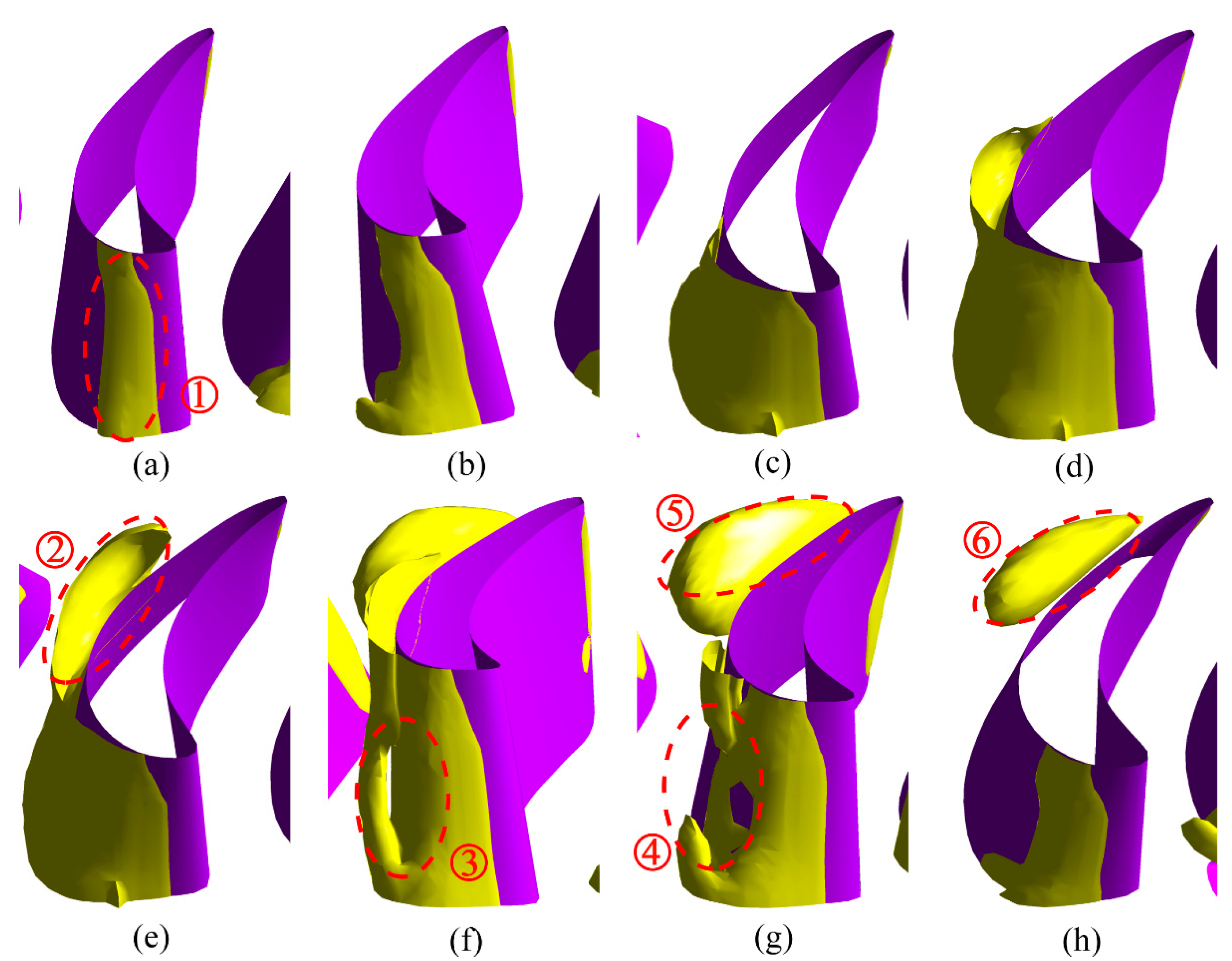
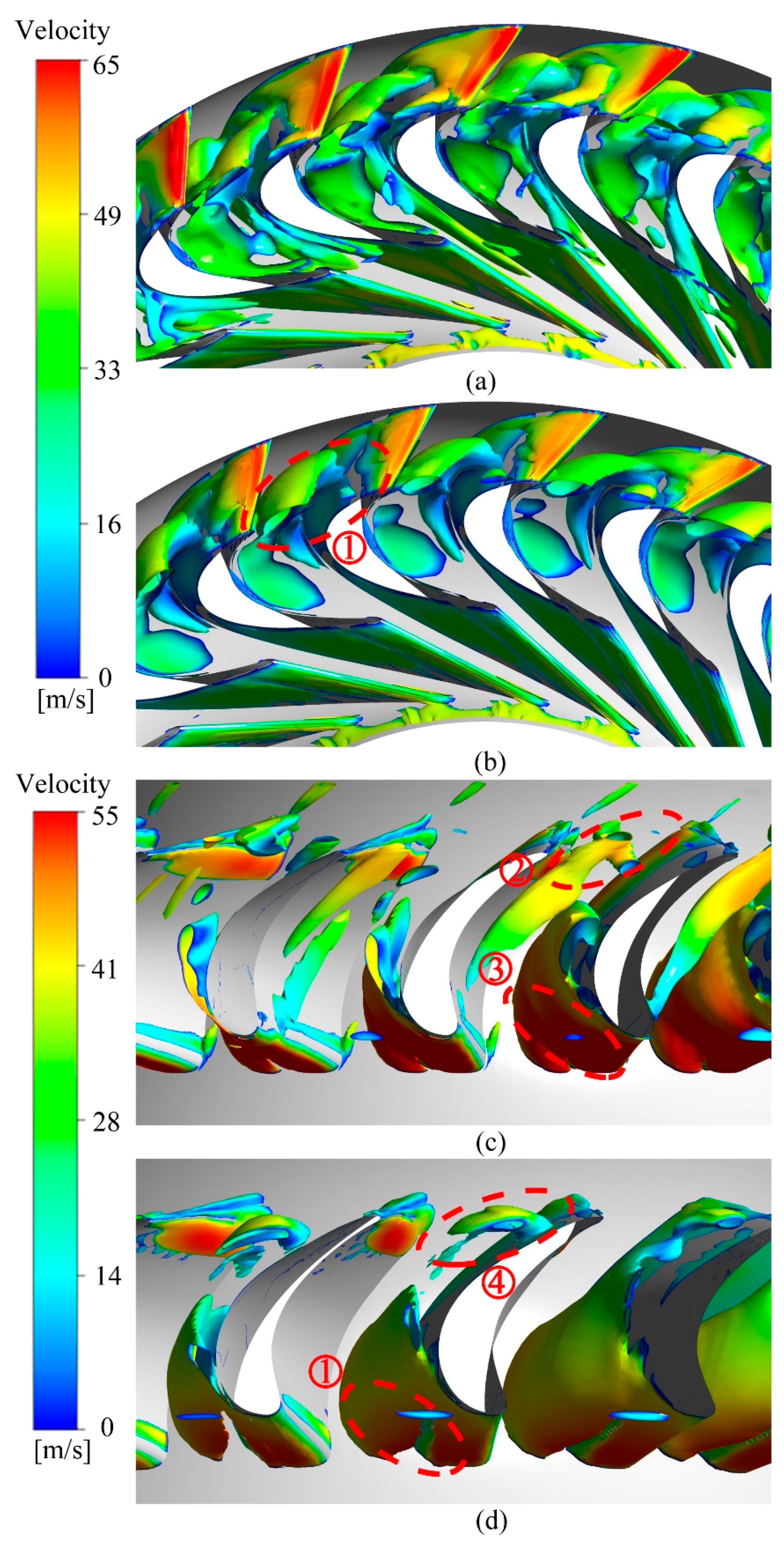
3.2. Transient Cavitation Behavior in the Hydrodynamic Torque Converter under the Stall Operating Condition

Heavy cavitation was predicted by the calculations in the stator under the stall operating condition, and only sheet cavitation was detected in the turbine. The fluid coming out of the turbine struck the stator blade with a large incidence angle, which resulted in a local high-velocity and low-pressure region on the suction surface near the leading edge and a large reverse flow downstream. The reattachment point of the reverse flow was located approximately 0.38 of the blade length, which was induced by a local reverse pressure gradient. Figure 7 depicts the periodic behavior of stator cavitation under the stall operating condition, which indicates vapor shedding and confirms that the reentrant jet shedding mechanism was captured well using the CFD models. The cavitation shedding was triggered by a reentrant jet, which formed upstream of the reattachment point of the reverse flow and was then driven by the reverse pressure gradient to move upstream toward the leading edge. The attached cavitation cloud finally detached, and the process repeated.
The height of the attached cavitation cloud at the leading edge increased with cavitation development, which can aggravate its unsteadiness. O-shaped cavitation was predicted at the peak of the attached cavitation near the stator leading edge, which has not previously been discovered by other researchers studying cavitation in hydrodynamic torque converters. Bin Ji and Cheng Liu at Wuhan University and the Beijing Institute of Technology, respectively, have similarly been researching hydrofoil cavitation, and they predicted shedding horseshoe cavitation and U-type cavitation [27,28]. With the further development of the reentrant jet, the O-type cavitation broke, and the attached cavitation was cut off. The occurrence of stator cavitation was determined by the circulation flow rate and incidence angle. When the circulation flow rate approached the threshold for cavitation inception, the attached cavitation was predicted in the hydrodynamic torque converter. Cavitation then became unstable with increasing mass flow rate, and the reentrant jet driven by the reverse pressure gradient moved towards the stator nose. The jet then lifted and cut off the attached cavitation, which triggered the shedding cycle. O-type cavitation could be predicted at the stator leading edge when the mass flow rate fulfilled certain conditions. The stator cavitation showed three forms depending on the reentrant jet, i.e., attached, O-type, and shedding cavitation. Four stages, i.e., inception, development, shedding, and collapse were observed.
The Q criterion was introduced to capture the vortex structure in the internal flow field [29], which is defined by
Q = 1 2 ( Ω 2 S 2 ) ,
where Ω (vortex tensor) and S (strain rate tensor) are the antisymmetric and symmetric portions, respectively, of the velocity gradient tensor.
Figure 8 depicts the vortex structure near the turbine and stator blades. The details of the turbulent flow are given under non-cavitation and cavitation conditions. The attached cavitation at the turbine leading edge induced a large-scale shedding vortex and significantly modified the structure of the local vortex. The fluid velocity on the leading edge of turbine was greater without cavitation than with cavitation. It indicated that the flow velocity without cavitation effects was overestimated. It is the result of blockage of the flow passage caused by cavitation bubbles. Because of the fully developed turbulence, the vortex structure of the turbine was scattered and chaotic when cavitation effects were not included, as shown in Figure 8a. As shown in Figure 8c, a measurable separation vortex was predicted at the turbine leading edge due to the attached cavitation, and the largest-scale vortex structure appeared at the maximum camberline location of the turbine blade. As shown in Figure 8b,d, measurable vortex separation was predicted at the leading edge of the stator because of the reentrant jet splitting the attached cavitation; this was closely related to the shedding cavitation of the stator. In contrast, there was no obvious shedding and separation vortex structure in the stator domain when cavitation effects were not considered. In general, cavitation intensified the flow blockage effect, which reduced the mass flow rate and caused the boundary layer to separate. The velocity in the internal flow field was over-predicted without cavitation, which increased the prediction error for the hydrodynamic performance. The flow field with cavitation more truly reflected the interaction between the cavitation and vortex fields. This indicates that the cavitation and vortex structures generally demonstrated strong interdependence.
Figure 9 shows unsteady cavitation in the stator and turbine domains under the stall operating condition. There was no measurable cavitation in the pump domain, where the pressure was high because of the high rotation speed. The cavitation in the turbine domain can be classified as stable attached cavitation. The stator cavitation was an unstable cloud cavitation. Cavitation bubbles formed near the leading edge of the suction surface of the turbine blade, which could block the turbine flow passage and reduce TR0. The fluid coming out of the pump struck the turbine blade at a large incidence angle, which resulted in a local high-velocity region on the suction surface near the leading edge and induced cavitation in the turbine domain.

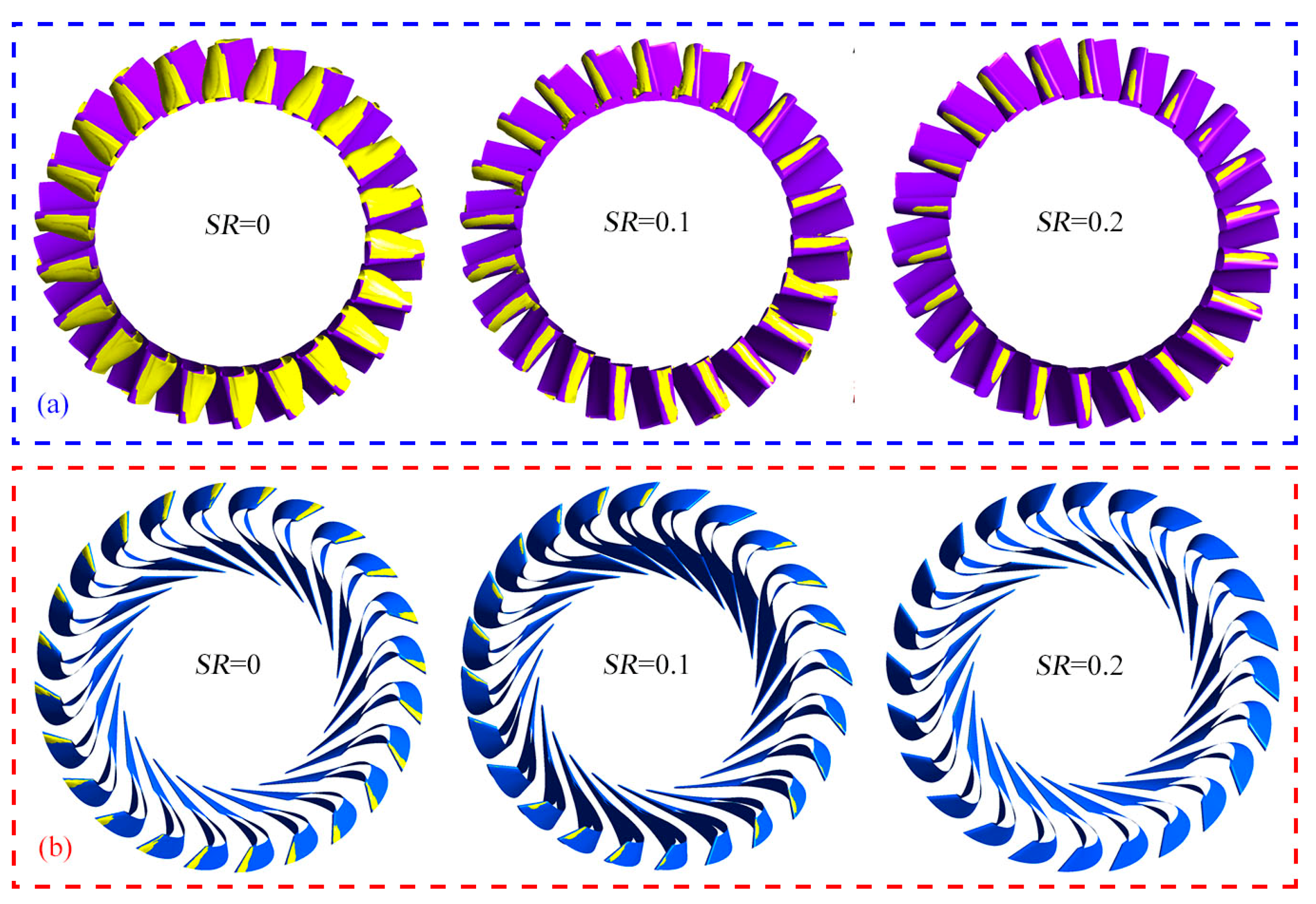
3.3. Cavitation Phenomena at Different SRs

Figure 10 shows the vapor volume fraction distribution in the hydrodynamic torque converter with cavitation. The cavitation bubbles in the turbine and stator domains decreased as the turbine rotation speed increased. When SR < 0.3, an unstable cloud cavitation was predicted within the stator, as shown in Figure 10a. When SR ≥ 0.3, there was no measurable cavitation in the stator because of the decreased mass flow rate. Stable attached cavitation developed in the turbine under the stall operating condition. When SR = 0.1, the cavitation bubbles became smaller and gradually vanished. When SR ≥ 0.2, the cavitation bubbles dissolved in the turbine, as shown in Figure 10b. These results indicate that no cavitation bubbles were generated in the pump under general operating conditions.

4. Cavitation Effects

4.1. Pressure Distribution on the Stator Blade Surface According to the Two CFD Models

Figure 11 shows the load distribution on the stator blade with and without cavitation. The torque resulted from the pressure difference between the suction surface and pressure surface of the blade. The fluid coming out of the turbine struck the leading edge of the stator, which caused a significant pressure drop at the suction side immediately downstream. Without cavitation, the predicted pressure on the suction side may even drop below zero, which indicates cavitation risk [30].The pressure difference between the pressure and suction sides was lower with cavitation than without cavitation, which was attributed to the negative pressure on the suction side being clipped by the vapor pressure. The pressure difference on the blade surface was over-predicted when cavitation was not considered, which explains the large prediction error for the hydrodynamic performance. It would be worth noting out that the vapor pressure is very small (about 10−4 MPa) so it is effectively zero in the figures.
To define the position of the monitoring points around the blade, x is the length of the curve between the points on the camberline and the leading edge of the blade. The intersection of the normal of the bisecting point on the camberline and the blade surface (the intersection point is the position of the blade surface y = 0) is considered and the outer normal of the blade surface is taken as the y direction at this intersection point, and the height of the monitoring point from the blade surface is y. c represents blade camberline length. The definition of camberline for blades can be found in Ref. [30]. The low-pressure region slowly shifted from x/c = −0.015–0.225 (SR = 0) to 0.018–0.217 (SR = 0.2). The cavitation center shifted from x/c = 0.106 to 0.142. These results indicate that the cavitation zone moved downstream of the suction surface of the stator blade as the SR increased. The mass flow rate coming out of the turbine and striking the stator blade decreased, which caused the flow stagnation point to transfer from the pressure side to the suction side. This increased the pressure on the suction side and reduced the risk of cavitation.

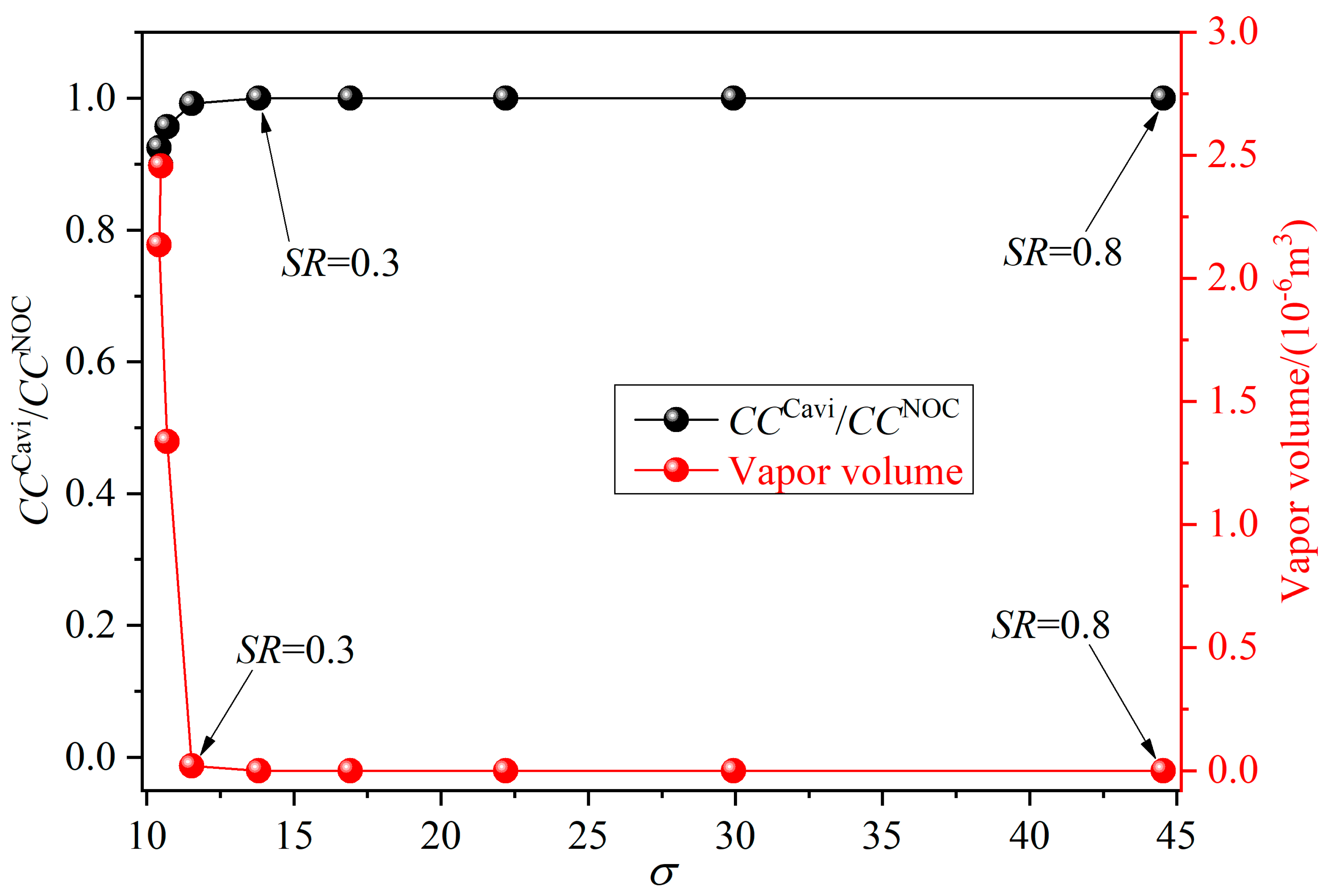
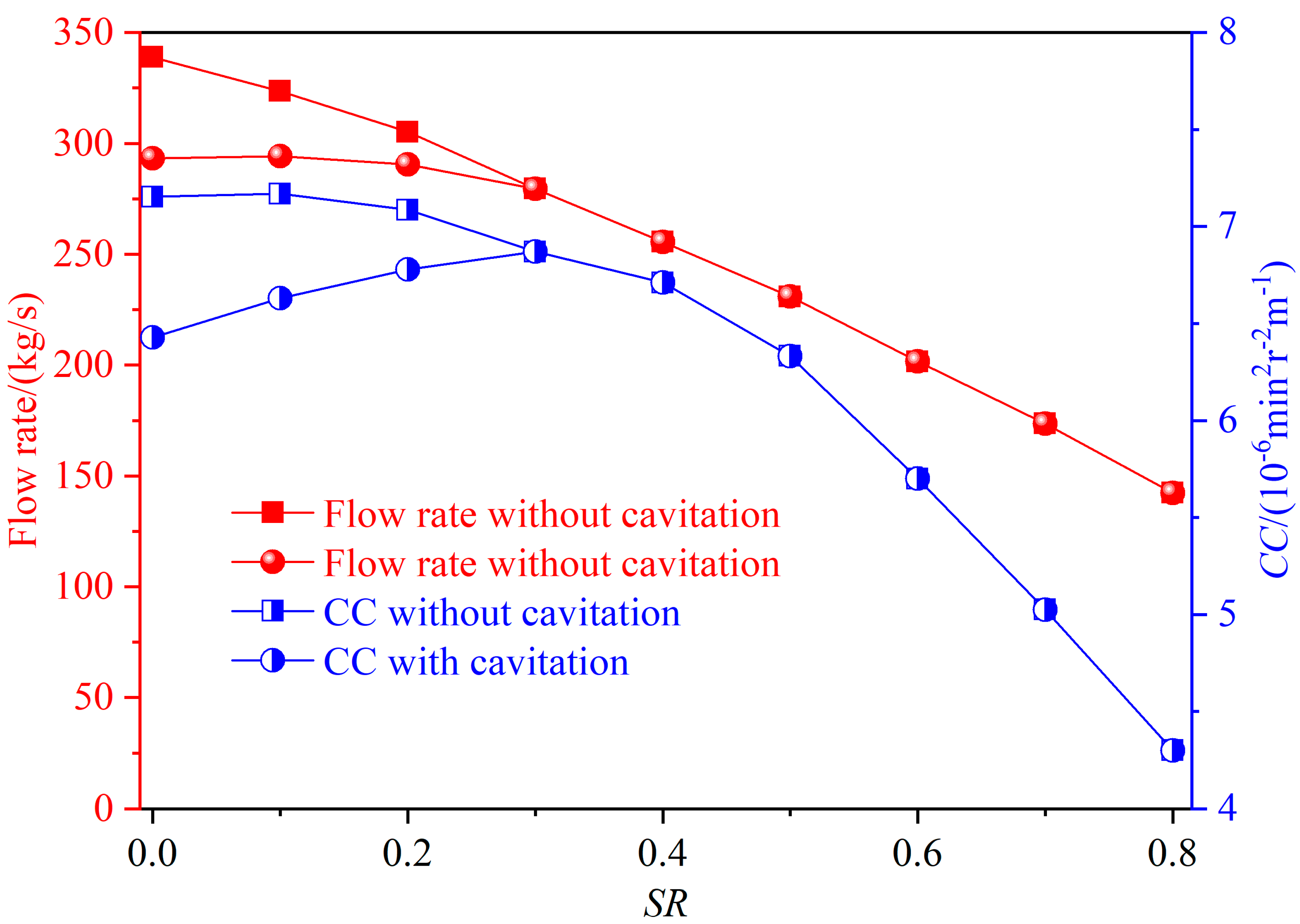
4.2. Mass Flow Rate and Capacity Loss in the Hydrodynamic Torque Converter

The dimensionless cavitation number σ was employed to evaluate the cavitation risk. A smaller cavitation number indicates greater cavitation risk. The cavitation number is defined by
σ = p r e f p v 0.5 ρ v r e f 2 ,
where p r e f , p v , and v r e f are the reference pressure (charge pressure), vapor pressure, and reference velocity, respectively. Mass flow rate represents the cyclic mass flowing through the torque converter per unit time, and specifically refers to the mass flow of the flow section at the inlet of the stator. For a hydrodynamic torque converter, the cavitation number is calculated by substituting v r e f with the average circumferential velocity ( U ) in the torus cross-section of the torque converter. This is defined using
U = m ˙ A ρ ,
where m ˙ is the circulating mass flow rate of the hydrodynamic torque converter. The mass flow rate depends on the cascade parameters and operating conditions. Therefore, the cavitation number comprehensively expresses the operating conditions, charge pressure, and cascade shape of the hydrodynamic torque converter. For a given torus design, A is constant. In this study, A was set to 2.56 × 10⁻² m2.
Figure 12 shows the relationship between the cavitation number and dimensionless capacity constant and vapor volume. The vapor volume decreased as the cavitation number increased. As the capacity constant approached unity, the influence of cavitation on the hydrodynamic performance and internal flow field decreased. When the cavitation number σ ≥ 10.5 (i.e., SR ≥ 0.3), cavitation had an almost negligible effect.
Figure 13 compares the mass flow rate and capacity constant with and without cavitation. Cavitation decreased the mass flow rate by nearly 50 kg/s under the stall operating condition, which reduced TR0 and CC0. The capacity constant and mass flow rate showed the same tendencies with and without cavitation at high SRs, which indicates that cavitation had disappeared.

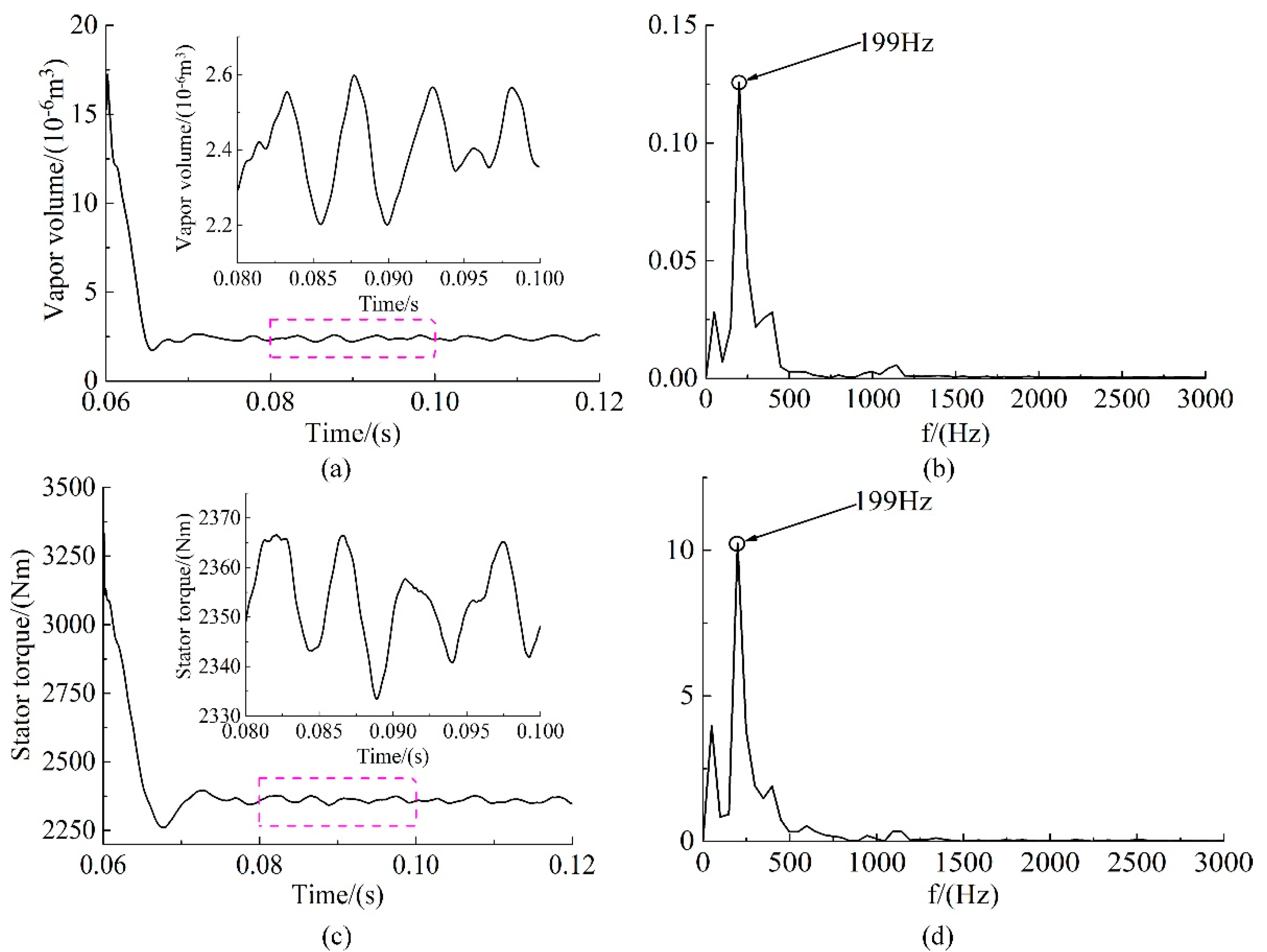
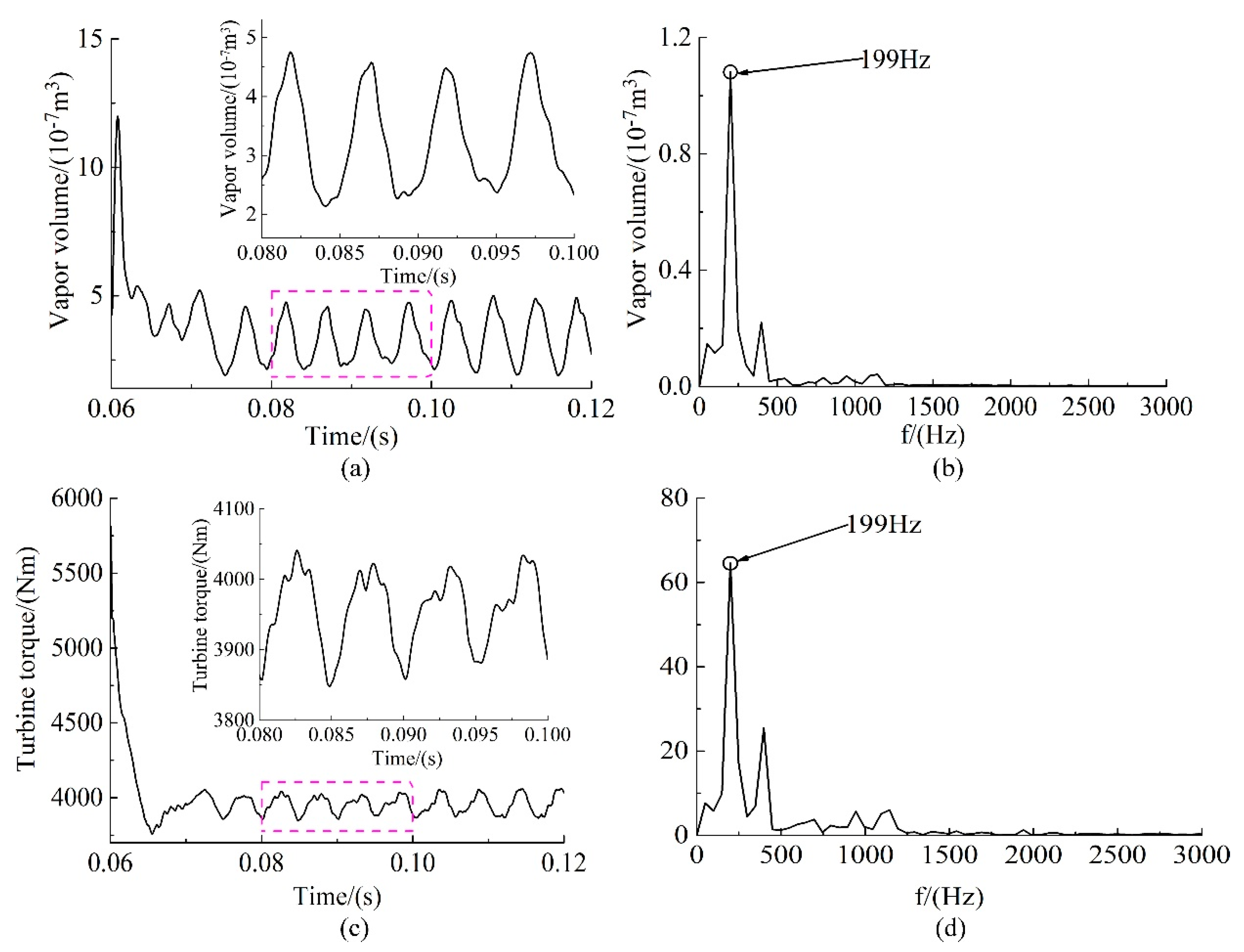
4.3. Spectral Analysis of the Stator and Turbine Torque

The vapor volume is a convenient parameter for understanding the transient behavior of cavitation flows [31,32]. In the stator, the evolution of the cavitation flow can be illustrated by the time history of the vapor volume. The variation of the vapor volume was periodic because of cavitation shedding from the suction side, as shown in Figure 14. The predicted cavitation shedding frequency was approximately 199 Hz. The O-type cavitation and shedding cavitation induced a variation of 0.24 × 10⁻⁶ m3 in the vapor volume in the stator domain, which degraded the hydrodynamic performance. The cavitation shedding frequency agreed well with the frequency of the stator torque, which indicates that the cavitation flow induced the vibration of the stator.
In the turbine, the evolution of the cavitation flow can be illustrated by the time history of the vapor volume. The vapor volume variation due to the rotor–stator interaction and turbine cavitation was periodic, as shown in Figure 15. The complicated cavitation processes may be attributed to the turbine blades, which are twisted in 3D. The cavitation frequency agreed well with the frequency of the turbine torque, which indicates that the cavitation flow induced the vibration of the turbine, as shown in Figure 15d. The turbine had the attached cavitation type, so the turbine torque was mainly attributed to the interaction between the pump and turbine. In addition, the attached cavitation shifted from the shell to the core with a non-uniform distribution, which induced instability. In general, the cavitation flow and torque demonstrated strong interdependence, and a cavitation flow induced vibration of the impeller torque.

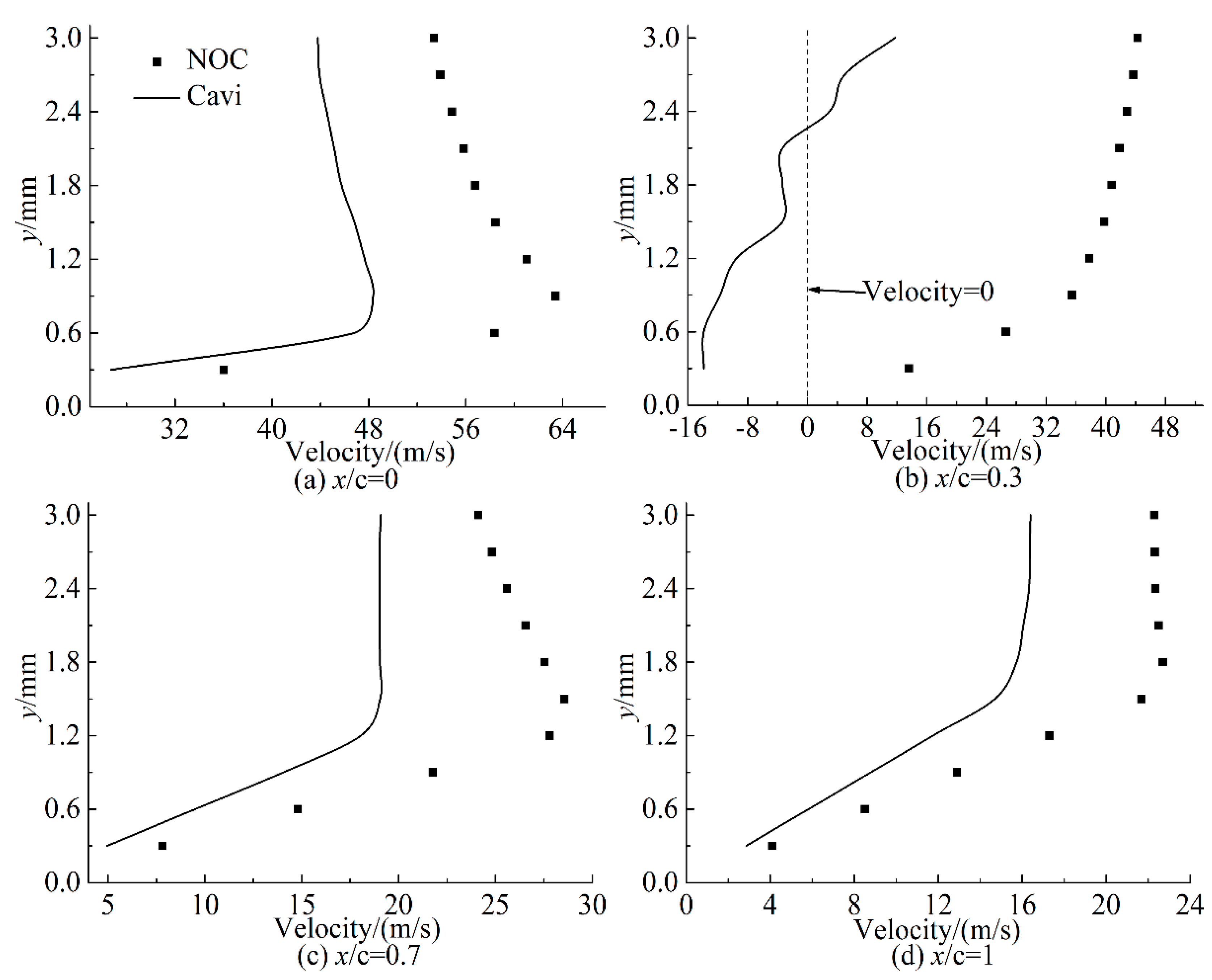
4.4. Normal Velocity Distribution at the Stator Surface with the Two CFD Models

The velocity field may illustrate the features of the cavitating flow and turbulence flow structure more directly. Figure 16 shows the normal velocity (The normal direction refers to the y direction, i.e., the outer normal direction of the blade surface. The stator blade is stationary, so the fluid velocity on the surface of the stator blade identical to 0.) distribution on the suction side of the stator blade under the stall operating condition. The normal velocities predicted by the two CFD models with and without cavitation were compared at different monitoring locations along the suction side. The velocity was greater without cavitation than with cavitation, which indicates that the velocity was over-predicted when cavitation was not considered. With cavitation, a measurable vortex at x/c = 0.3 of the blade length was observed, which was triggered by cavitation in the stator. The shedding cavitation in the stator was driven by the reverse pressure gradient, which blocked the flow passage. This indicates that cavitation in the stator intensified the flow blockage effect, which reduced the capacity constant and mass flow rate.

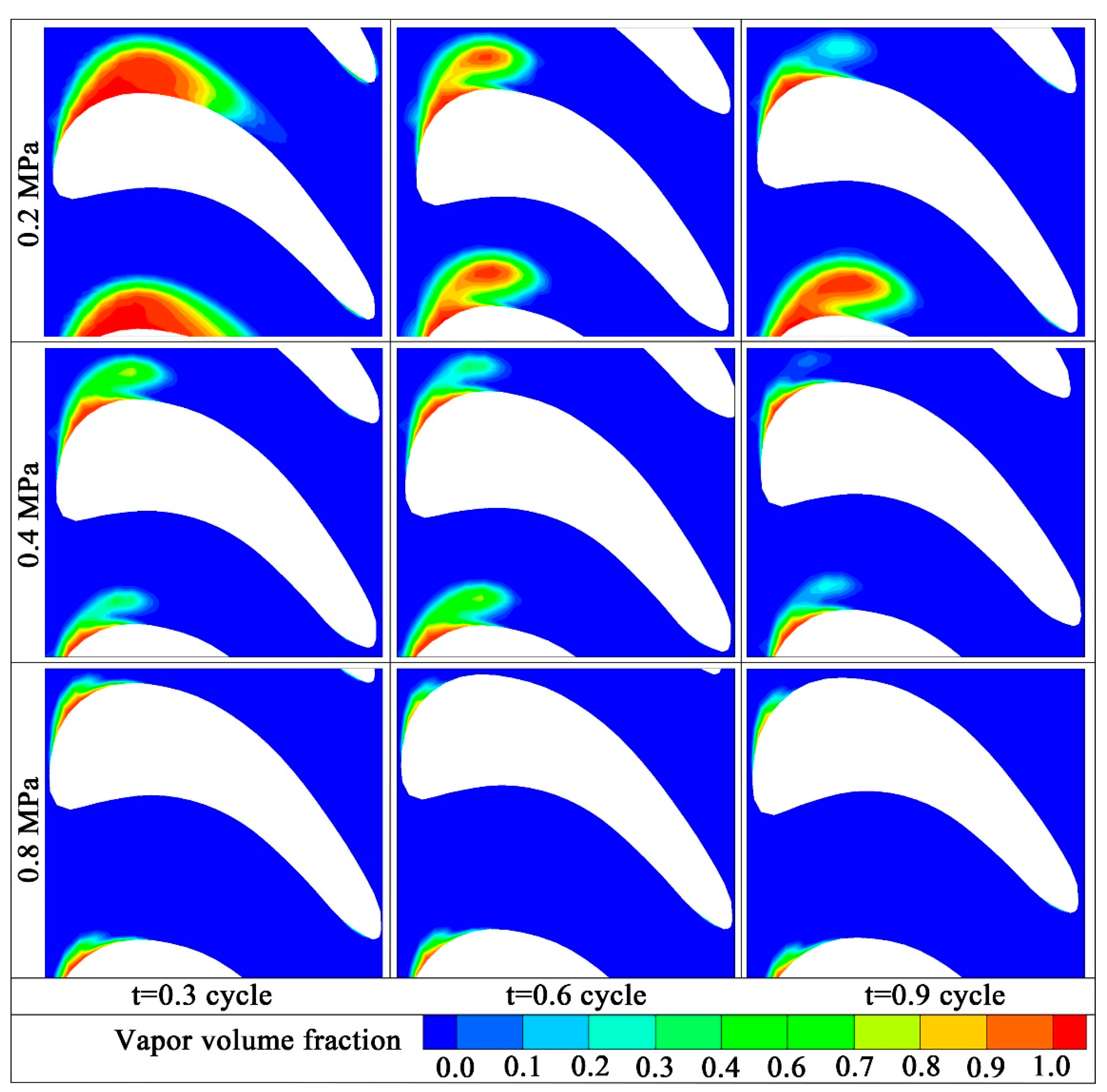
4.5. Effect of the Backpressure

Not only the inception and development of cavitation but also the backpressure conditions are important for inferring the cavitation control in a hydrodynamic torque converter. Figure 17 shows the vapor volume distribution in the stator of the hydrodynamic torque converter at different backpressures. The backpressure had a significant effect on both the cavitation intensity and stability. At a backpressure of 0.2 MPa, the cavitation reached its maximum intensity because the difference between the charge pressure and backpressure is greatest. The cavitation intensity decreased as the backpressure increased further. Only attached cavitation was predicted in the stator domain when the backpressure reached 0.8 MPa, at which point, the cavitation intensity in the stator reached its minimum. This indicates that the oil operating conditions are essential for controlling cavitation in turbomachinery.
Table 4 presents the vapor volume and cavitation number at different backpressures. The pressure difference between the charge pressure and backpressure decreased with increasing backpressure, and the pressure in the entire working chamber increased. The vapor volume gradually decreased with an increasing cavitation number. This indicates that a reasonable increase in the backpressure can significantly suppress the cavitation risk inside the hydrodynamic torque converter.

5. Conclusions

Due to the limited test equipment, the author could not study the cavitation behavior inside the torque converter through experiments. The cavitation behavior inside the torque converter calculated by the author through CFD can provide a reference for the research of turbomachine cavitation, and more accurate cavitation prediction needs to be verified by experiments. The transient turbulent and cavitation flow in a hydrodynamic torque converter was numerically investigated with a RANS turbulence model and Zwart–Gerber–Belamri cavitation model, and the simulation results were compared with experimental data. The proposed CFD model agreed well with the experimental data in Figure 6. The study focused on the evolution of cavitation and its effect on the torque characteristics, especially the formation and development of O-type cavitation and shedding cavitation structures around the stator blades. The following conclusions were made:
(1) Under non-cavitating flow conditions, the velocity and pressure were over-predicted, which increased the prediction error for the hydrodynamic performance. Especially under the stall operating condition, cavitation reduced the mass flow rate by nearly 50 kg/s, which reduced the capacity constant by 13.23%. With cavitation taken under consideration, the pressure below the saturated vapor threshold (110 Pa) was clipped out, which accurately reflects the interaction between the cavitation and vortex field in a hydrodynamic torque converter.
(2) Three cavitation forms (attached, O-type, and shedding) and four stages (inception, development, shedding, and collapse) were predicted in the stator because of the reverse reentrant jet. The reattachment point of the reverse flow was located at approximately x/c = 0.3 of blade length (dimensionless). The turbine cavitation was the attached type. There was significant interaction between the cavitation behavior and torque characteristics, and cavitation generated quasi-periodic fluctuations in the torque, where the cavitation shedding frequency was approximately 199 Hz. The results clarified the evolution of cavitation and the cavitation mechanism at low SRs, and they provide a theoretical reference for the optimal design of hydrodynamic torque converters with a high power density. When SR ≤ 0.1, cavitation mainly occurred in the turbine and stator domains, and no measurable cavitation was predicted in the pump domain where high pressure was dominant owing to the high rotation speed. When 0.1 < SR < 0.3, cavitation only occurred in the stator domain. When SR ≥ 0.3, visible cavitation bubbles disappeared, and cavitation had almost no effect on the hydrodynamic performance.
(3) The pressure of the working chamber increased with the backpressure, which reduced the cavitation risk. Thus, increasing the working chamber pressure appears to be an effective measure for suppressing cavitation in turbomachinery. The torque converter should be designed to increase the backpressure and decrease the pressure difference between the charge pressure and backpressure, which can significantly improve the cavitation suppression effect.
The cavitation suppression measures considered in this study were limited. Future work should consider the effectiveness of varying the charge pressure, backpressure, charge pressure and backpressure location configurations, cascade parameters, and suppression slot.

Author Contributions

Conceptualization, W.M. and C.L.; methodology, W.M.; software, Z.R.; validation, Z.R. and C.L.; formal analysis, C.L.; investigation, Z.R.; resources, W.M.; data curation, Z.R.; writing—original draft preparation, Z.R.; writing—review and editing, W.M.; visualization, Z.R.; supervision, W.M.; project administration, W.M.; funding acquisition, C.L. All authors have read and agreed to the published version of the manuscript.

Funding

This work was supported by the Key Scientific and Technological Project of Jilin Province (grant no. 20170204066GX) and the Natural Science Foundation of Jilin Province “Multidisciplinary Collaborative Optimization Design Theory of Vehicle Hydraulic Retarder with Cavitation Effect” (grant no. 20200201222JC).

Data Availability Statement

The data presented in this study are available on request from the Corresponding author.

Conflicts of Interest

The authors declare no conflict of interest.

Nomenclature

S R speed ratio
D hydrodynamic torque converter torus diameter, mm
N Turbine turbine rotation speed, rpm
N Pump pump rotation speed, rpm
T Turbine turbine torque, Nm
T Pump pump torque, Nm
T R torque ratio
C C capacity constant, 10−6 min 2 r 2 m 1
η efficiency
p c charge pressure, Pa
α l liquid volume fraction
ρ l liquid density, kg m−3
v velocity, m s−1
m ˙ mass flow rate, kg s−1
R B bubble radius, m
p v vapor pressure, Pa
p mixture pressure, Pa
α v vapor volume fraction
ρ v vapor density, kg m−3
α nuc volume fraction of the nucleation site
F vap vaporization constant
F cond condensation constant
ρ m mixture density, kg m−3
μ m mixture dynamic viscosity, Pa s
μ l liquid dynamic viscosity, Pa s
μ v vapor dynamic viscosity, Pa s
σ cavitation number
p r e f reference pressure, Pa
v r e f reference velocity, m s−1
cblade camberline length, mm
List of Sub-Indices
Testtest data
NOCnon-cavitation CFD results
Cavicavitation CFD results

References

  1. Liu, C.; Li, J.; Bu, W.; Ma, W.; Shen, G.; Yuan, Z. Large eddy simulation for improvement of performance estimation and turbulent flow analysis in a hydrodynamic torque converter. Eng. Appl. Comput. Fluid Mech. 2018, 12, 635–651. [Google Scholar] [CrossRef] [Green Version]
  2. Flack, R.; Brun, K. Fundamental analysis of the secondary flows and jet-wake in a torque converter pump—Part 1: Model and flow in a rotating passage. ASME J. Fluids Eng. 2003, 127, 1183–1191. [Google Scholar]
  3. Wu, G.Q.; Wang, L.J. Application of dual-blade stator to low-speed ratio performance improvement of torque converters. China J. Mech. Eng. 2016, 29, 293–300. [Google Scholar] [CrossRef]
  4. Bakir, F.; Rey, R.; Gerber, A.G.; Belamri, T.; Hutchinson, B. Numerical and experimental investigations of the cavitating behavior of an inducer. Int. J. Rotating Mach. 2007, 10, 15–25. [Google Scholar] [CrossRef] [Green Version]
  5. Brennen, C.E. A review of the dynamics of cavitating pumps. ASME J. Fluids Eng. 2012, 135, 301–311. [Google Scholar] [CrossRef]
  6. Park, S.I.; Lee, S.J.; You, G.S.; Suh, J.C. An experimental study on tip vortex cavitation suppression in a marine propeller. J. Ship Res. 2014, 58, 157–167. [Google Scholar] [CrossRef]
  7. Tsutsumi, K.; Watanable, S.; Tsuda, S.; Yamaguchi, T. Cavitation simulation of automotive torque converter using a homogeneous cavitation model. Eur. J. Mech. B Fluids 2016, 61, 263–270. [Google Scholar] [CrossRef] [Green Version]
  8. Zhang, D.S.; Shi, L.; Shi, W.D. Numerical simulation and experimental study on impeller tip region cavitation in axial flow pump. J. Hydraul. Eng. 2014, 45, 335–342. [Google Scholar]
  9. Bilus, I.; Predin, A. Numerical and experimental approach to cavitation surge obstruction in water pump. Int. J. Numer. Methods Heat Fluid Flow 2009, 19, 818–834. [Google Scholar] [CrossRef]
  10. Feng, X.R.; Lu, J.M. Effects of balanced skew and biased skew on the cavitation characteristics and pressure fluctuations of the marine propeller. Ocean. Eng. 2019, 184, 184–192. [Google Scholar] [CrossRef]
  11. Anderson, C.L.; Zeng, L.; Sweger, P.O.; Narain, A.; Blough, J.R. Experimental Investigation of Cavitation Signatures in an Automotive Torque Converter Using a Microwave Telemetry Technique. Int. J. Rotating Mach. 2003, 9, 403–410. [Google Scholar] [CrossRef] [Green Version]
  12. Mekkes, J.; Anderson, C.; Narain, A. Static Pressure Measurements and Cavitation Signatures on the Nose of a Torque Converter’s Stator Blades. In Proceedings of the 10th International Symposium on Rotating Machinery (ISROMAC-10), Honolulu, HI, USA, 7–11 March 2004. Paper no. ISROMAC10-2004-035. [Google Scholar]
  13. Kowalski, D.; Anderson, C.; Blough, J. Cavitation Detection in Automotive Torque Converters Using Nearfield Acoustical Measurements. SAE Trans. 2005, 114, 2796–2804. [Google Scholar]
  14. Foeth, E.J.; Van Doorne, C.W.H.; Van Terwisga, T.; Wieneke, B. Time resolved PIV and flow visualization of 3D sheet cavitation. Exp. Fluids 2006, 40, 503–513. [Google Scholar] [CrossRef]
  15. Kravtsova, A.Y.; Markovich, D.M.; Pervunin, K.S.; Timoshevskiy, M.; Hanjalić, K. High-speed visualization and PIV measurements of cavitating flows around a semi-circular leading-edge flat plate and NACA0015 hydrofoil. Int. J. Multiph. Flow 2014, 60, 119–134. [Google Scholar] [CrossRef]
  16. Kravtsova, A.Y.; Markovich, D.M.; Pervunin, K.S.; Timoshevskii, M.V.; Hanjalić, K. Cavitation on a semicircular leading-edge plate and NACA0015 hydrofoil: Visualization and velocity measurement. Therm. Eng. 2014, 61, 1007–1014. [Google Scholar] [CrossRef]
  17. Kravtsova, A.Y.; Markovich, D.M.; Pervunin, K.S.; Timoshevskiy, M.V. High-speed imaging and PIV measurements in turbulent cavitating flows around 2D hydrofoils. In International Symposium on Turbulence and Shear Flow Phenomena (TSFP); Elsevier: Amsterdam, Netherlands, 2013; Paper No. TSFP, 2. [Google Scholar]
  18. Robinette, D.; Anderson, C.; Blough, J.; Johnson, M.; Maddock, D.; Schweitzer, J. Characterizing the Effect of Automotive Torque Converter Design Parameters on the Onset of Cavitation at Stall. SAE Trans. 2007, 116, 1735–1746. [Google Scholar]
  19. Robinette, D.L.; Schweitzer, J.M.; Maddock, D.G.; Anderson, C.L.; Blough, J.R.; Johnson, M.A. Predicting the Onset of Cavitation in Automotive Torque Converters—Part I: Designs with Geometric Similitude. Int. J. Rotating Mach. 2008, 2008, 1–8. [Google Scholar] [CrossRef] [Green Version]
  20. Robinette, D.L.; Schweitzer, J.M.; Maddock, D.G.; Anderson, C.L.; Blough, J.R.; Johnson, M.A. Predicting the Onset of Cavitation in Automotive Torque Converters—Part II: A Generalized Model. Int. J. Rotating Mach. 2008, 2008, 1–8. [Google Scholar] [CrossRef] [Green Version]
  21. Watanabe, S.; Otani, R.; Kunimoto, S.; Hara, Y.; Furukawa, A.; Yamaguchi, T. Vibration Characteristics due to Cavitation in Stator Element of Automotive Torque Converter at Stall Condition. In ASME Fluids Engineering Division Summer Meeting (FEDSM); ASME: New York, NY, USA; Rio Grande, PR, USA, 2013; pp. 535–541. [Google Scholar]
  22. Ju, J.; Jang, J.; Choi, M.; Baek, J.H. Effects of Cavitation on Performance of Automotive Torque Converter. Adv. Mech. Eng. 2016, 8, 1–9. [Google Scholar] [CrossRef] [Green Version]
  23. Liu, C.; Wei, W.; Yan, Q.; Weaver, B.K. Torque converter capacity improvement through cavitation control by design. ASME J. Fluids Eng. 2017, 139, 1101–1110. [Google Scholar] [CrossRef]
  24. Zwart, P.J.; Gerber, A.G.; Belamri, T. A Two-Phase Flow Model for Predicting Cavitation Dynamics. In Fifth International Conference on Multiphase Flow; Elsevier: Yokohama, Japan, 2004. [Google Scholar]
  25. Singhal, A.K.; Athavale, M.M.; Li, H.; Jiang, Y. Mathematical basis and validation of the full cavitation model. ASME J. Fluids Eng. 2002, 124, 617–624. [Google Scholar] [CrossRef]
  26. Liu, C.B.; Liu, C.S.; Ma, W.X. Mathematical model for elliptic torus of automotive torque converter and fundamental analysis of its effect on performance. Math. Probl. Eng. 2015, 2015, 1–13. [Google Scholar] [CrossRef]
  27. Long, X.P.; Cheng, H.Y.; Ji, B.; Arndt, R.E.; Peng, X. Large eddy simulation and Euler-Lagrangian coupling investigation of the transient cavitating turbulent flow around a twisted hydrofoil. Int. J. Multiph. Flow 2018, 100, 41–56. [Google Scholar] [CrossRef]
  28. Liu, C.; Yan, Q.D.; Wood, H.G. Numerical investigation of passive cavitation control using a slot on a three-dimensional hydrofoil. Int. J. Numer. Methods Heat Fluid Flow 2020, 30, 3585–3605. [Google Scholar] [CrossRef]
  29. Dubief, Y.; Delcayre, F. On coherent-vortex identification in turbulence. J. Turbul. 2000, 1, 1–12. [Google Scholar] [CrossRef]
  30. Liu, C.; Wei, W.; Yan, Q.D.; Weaver, B.K.; Wood, H.G. Influence of stator blade geometry on torque converter cavitation. ASME J. Fluids Eng. 2018, 140, 1101–1110. [Google Scholar] [CrossRef]
  31. Ji, B.; Luo, X.W.; Wu, Y.L.; Peng, X.; Duan, Y. Numerical analysis of unsteady cavitating turbulent flow and shedding horse-shoe vortex structure around a twisted hydrofoil. Int. J. Multiph. Flow 2013, 51, 33–43. [Google Scholar] [CrossRef] [Green Version]
  32. Ji, B.; Luo, X.W.; Wang, X.; Peng, X.; Wu, Y.; Xu, H. Unsteady numerical simulation of cavitating turbulent flow around a highly skewed model marine propeller. ASME J. Fluids Eng. 2011, 133, 1101–1108. [Google Scholar] [CrossRef]
Figure 1. Cavitation in typical turbomachines. (a) cavitation generated in inducer, (b) cavitation in tip vortices and marine propeller blades, (c) cavitation damage of a marine propeller blade, and (d) cavitation generated in hydrodynamic torque converter.
Applsci 11 02798 g001
Figure 2. Flow passage layout of the hydrodynamic torque converter. (a) torus meridian view and (b) single flow passage (1-pump domain, 2-turbine domain, 3-stator domain, 4-P-T clearance domain, 5-T-S clearance domain, and 6-S-P clearance domain).
Applsci 11 02798 g002
Figure 3. Hydrodynamic torque converter cross-section view (1-pump, 2-turbine, and 3-stator).
Applsci 11 02798 g003
Figure 4. Structural mesh model of the hydrodynamic torque converter.
Applsci 11 02798 g004
Figure 5. Predicted torque results under variant element density (speed ratio (SR) = 0).
Applsci 11 02798 g005
Figure 6. Comparison of computational fluid dynamics (CFD) results against test data under various operating conditions.
Applsci 11 02798 g006
Figure 7. Unsteady cavitation process in the stator domain under SR = 0 condition. (a) t = 0.125 T, (b) t = 0.25 T, (c) t = 0.375 T, (d) t = 0.5 T, (e) t = 0.625 T, (f) t = 0.75 T, (g) t = 0.875 T, and (h) t = 1 T. (1-attached cavity, 2-cavity development, 3-“O” type cavity, 4-“O” type cavity break, 5-shedding cavity, and 6-scatter cavity (collapse)).
Applsci 11 02798 g007
Figure 8. Vortex distribution near the turbine and stator blades under non-cavitation and cavitation conditions (Q = 2.4085 × 10⁶ s−2). (a) vortex distribution without cavitation (turbine), (b) vortex distribution with cavitation (turbine), (c) vortex distribution without cavitation (stator), and (d) vortex distribution with cavitation (stator). (1-separation vortex, 2-scatter vortex, 3-attached vortex, and 4-shedding vortex, (SR = 0).
Applsci 11 02798 g008
Figure 9. Unsteady cavitation in the stator (left) and the turbine (right) domain under SR = 0 condition.
Applsci 11 02798 g009
Figure 10. Isosurface of 0.1 vapor volume fraction distribution in the stator and turbine domains under various SRs. (a) cavitation distribution in stator at different SRs, (b) cavitation distribution in turbine at different SRs.
Applsci 11 02798 g010
Figure 11. Stator blade load distributions with cavitation and non-cavitation at different SRs.
Applsci 11 02798 g011
Figure 12. Non-dimensional capacity constant and vapor volume under various dimensionless cavitation numbers ( σ ).
Applsci 11 02798 g012
Figure 13. Mass flow rate and capacity constant caused by cavitation at various SRs.
Applsci 11 02798 g013
Figure 14. Variations in the vapor volume and torque of the stator in the time and frequency domains (SR = 0): (a) vapor volume, (b) vapor volume spectrum, (c) torque, and (d) torque spectrum.
Applsci 11 02798 g014
Figure 15. Variations in the vapor volume and torque of the turbine in the time and frequency domains (SR = 0): (a) vapor volume, (b) vapor volume spectrum, (c) torque, and (d) torque spectrum.
Applsci 11 02798 g015
Figure 16. Normal velocity distributions at selected monitoring locations along the suction side of the stator under non-cavitation and cavitation conditions (SR = 0).
Applsci 11 02798 g016
Figure 17. Vapor volume fraction distributions for one typical cycle with different backpressures (SR = 0).
Applsci 11 02798 g017
Table 1. Constant coefficients in the shear stress transport (SST) k–ω model.
β * α 1 β 1 σ k 1 σ ω 1 α 2 β 2 σ k 2 σ ω 2
0.095/93/400.850.50.440.082810.856
Table 2. Detailed computational fluid dynamics (CFD) model settings.
Analysis TypeTransient
Fluid properties ρ l = 860 kg m−3, μ l = 0.0258 Pa s
Vapor properties ρ v = 2.1 kg m−3, μ v = 1.2 × 10⁻⁵ Pa s
Turbulence modelSST k–ω
Advection schemeHigh resolution
Convergence targetRMS 1 × 10⁻⁴
Pump statusFixed at 2000 rpm
Turbine statusVariable within 0–1600 rpm
Stator statusStationary
Charge pressure0.8 MPa
Backpressure0.4 MPa
Transient formulationSecond-order upwind
Other term spatial discretizationSecond-order upwind
Time step1 × 10−4 s
Boundary detailsNo slip and smooth wall
Vapor pressure ( p v )110 Pa
Table 3. Structural parameters of the hydrodynamic torque converter.
ElementInlet AngleOutlet AngleNumber of Blades
Pump123°64°29
Turbine32°157°24
Stator120°33°22
Table 4. Cavitation numbers under various backpressure conditions.
Charge Pressure (MPa)Backpressure (MPa)Vapor Volume (10−6 m3)Mass Flowrate (kg s−1)Cavitation Number
0.80.24.1827145308.504469.474
0.80.42.46293.3139510.480
0.80.62.4342955287.0004110.946
0.80.81.8027153277.2430411.731
Publisher’s Note: MDPI stays neutral with regard to jurisdictional claims in published maps and institutional affiliations.

