
Object Detection, Distributed Cloud Computing and Parallelization Techniques for Autonomous Driving Systems


 ,
,  and
and 
Abstract
Featured Application
Abstract
1. Introduction
2. Background
2.1. Feature Extraction Methods used for Object Detection in AVs
2.1.1. Camera-Based
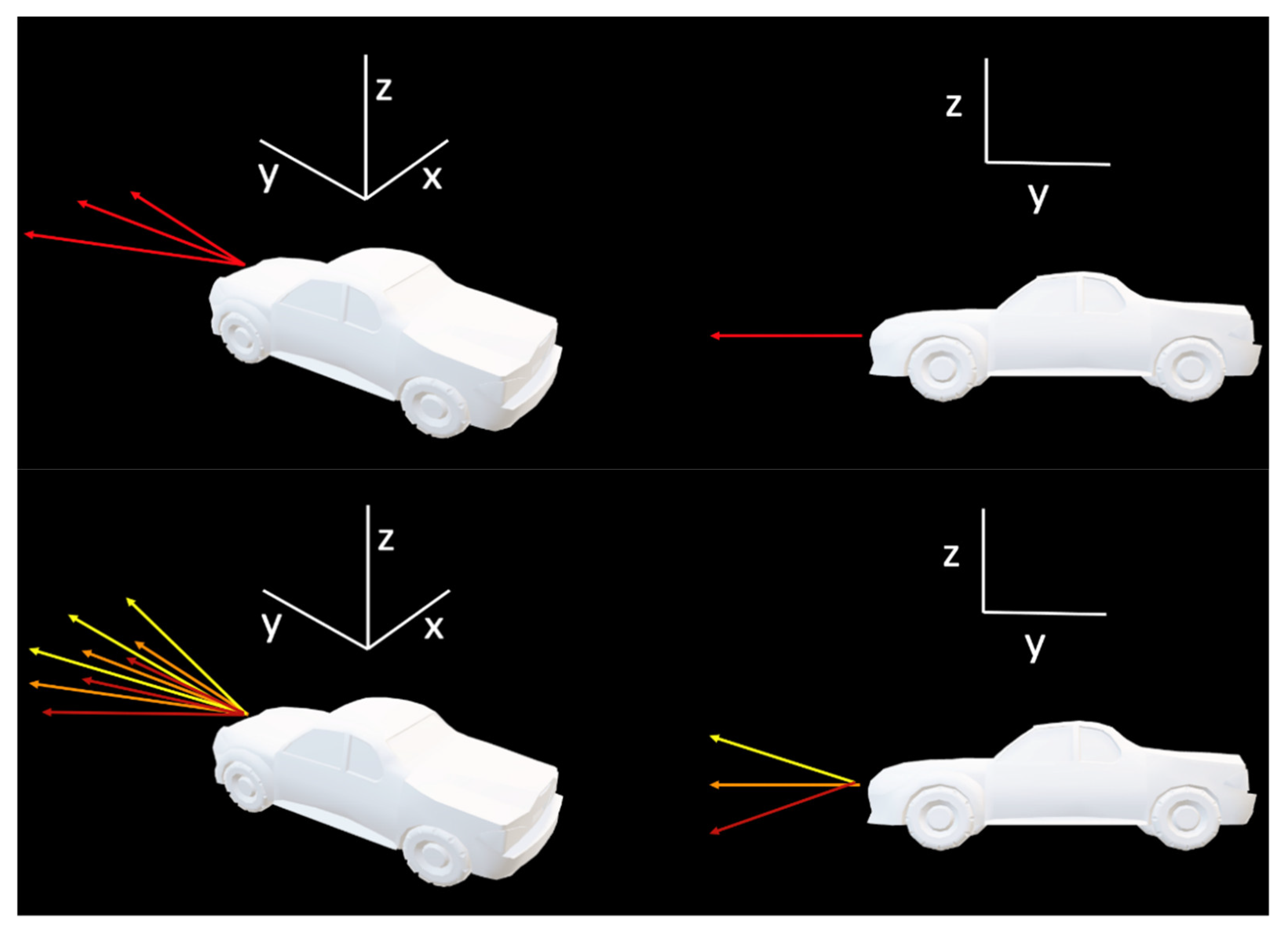
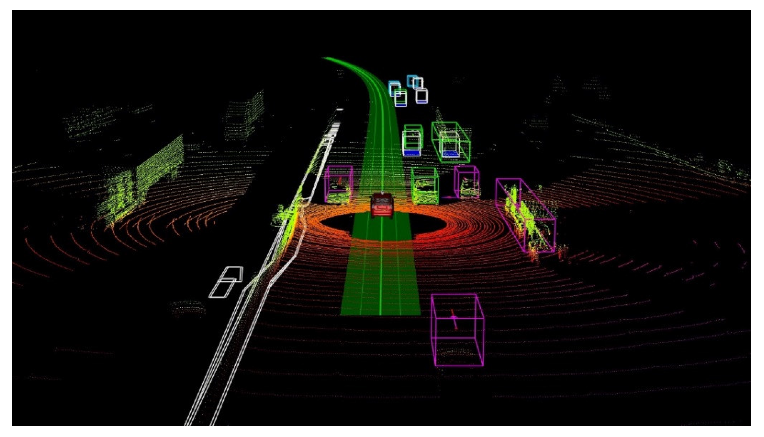
2.1.2. LiDAR-Based
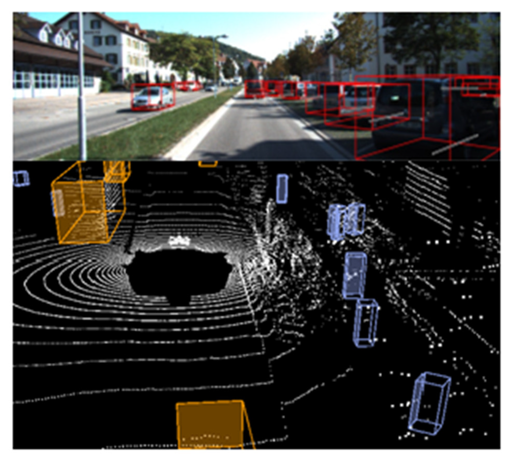
2.1.3. Hybrid Approaches
2.2. Object Detection
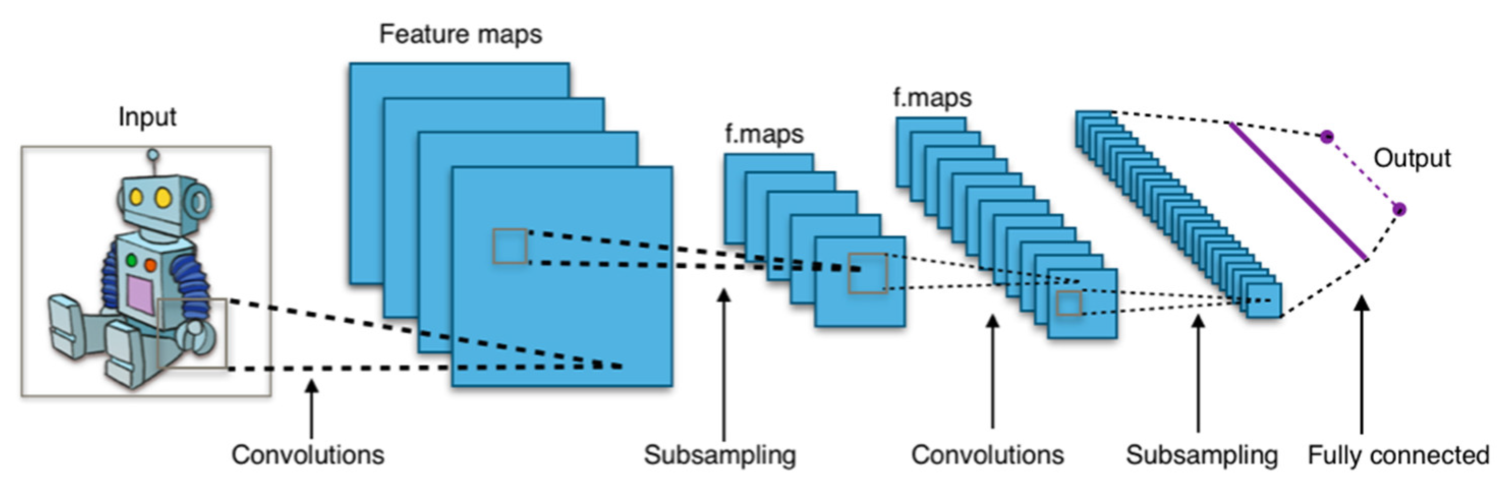
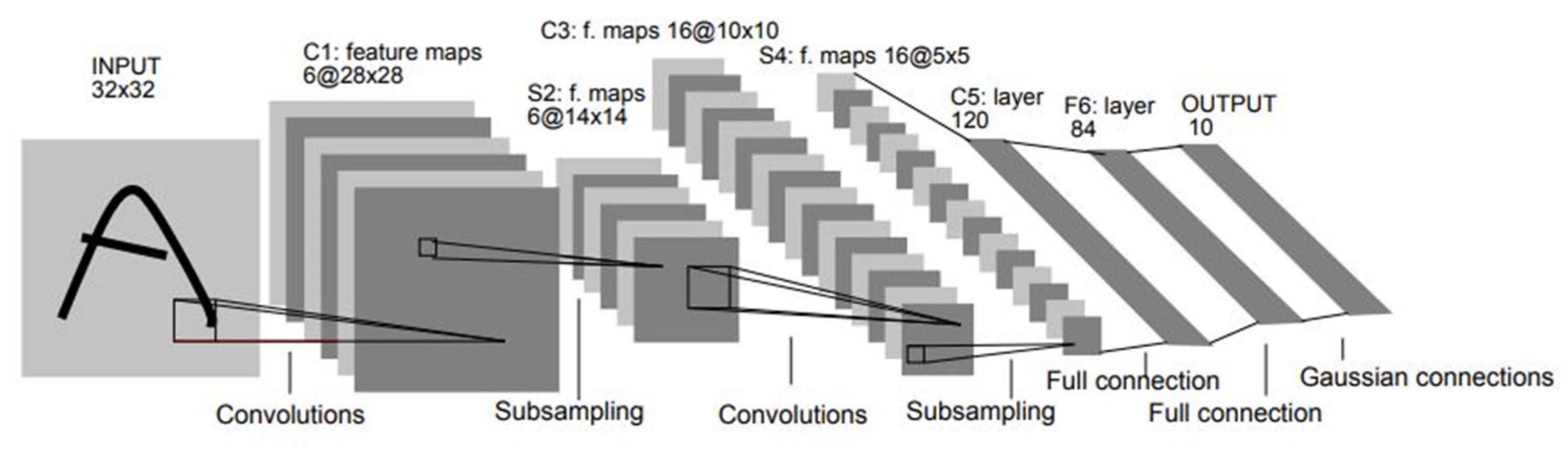
2.2.1. Convolutional Neural Network (CNN)
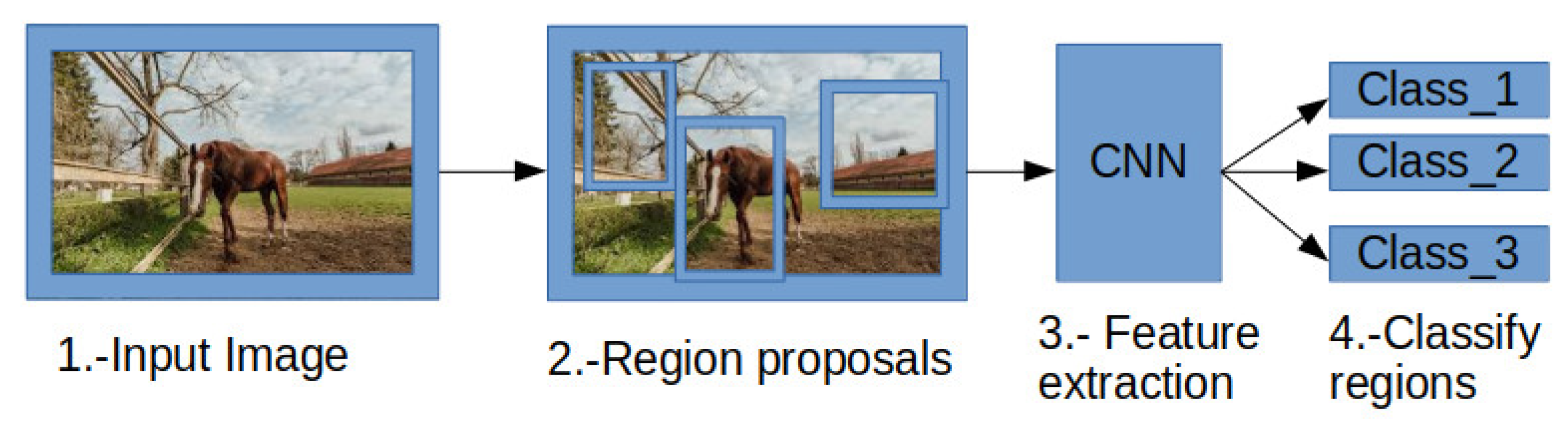
2.2.2. R-CNN
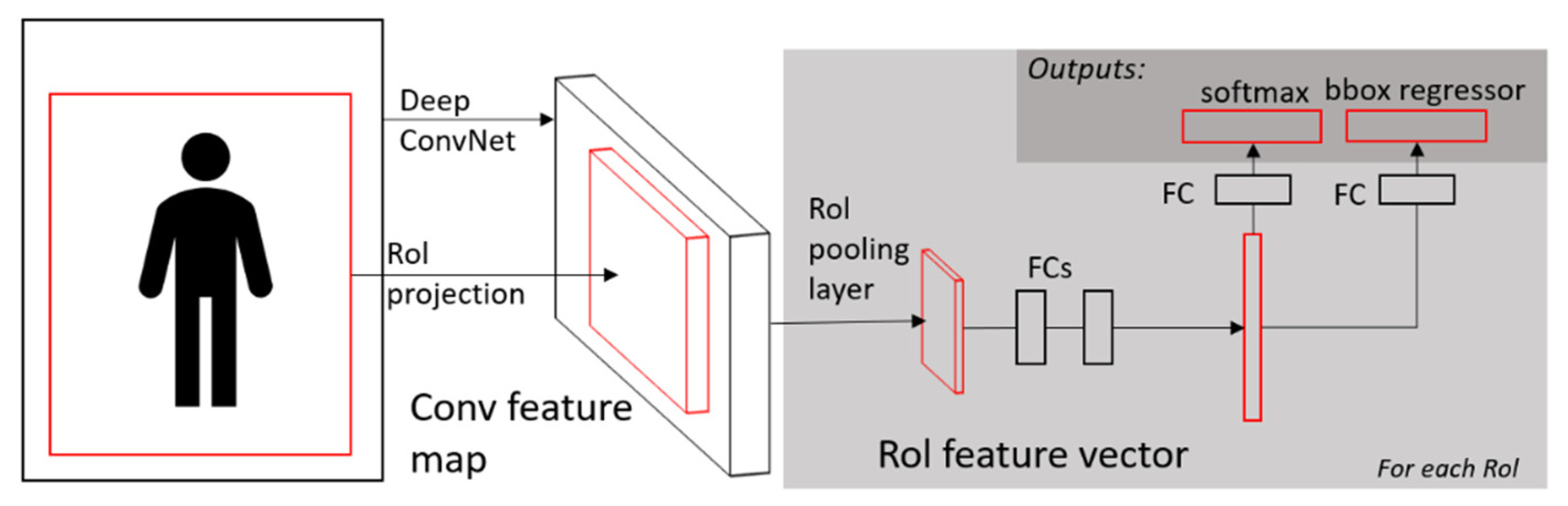
2.2.3. Fast R-CNN
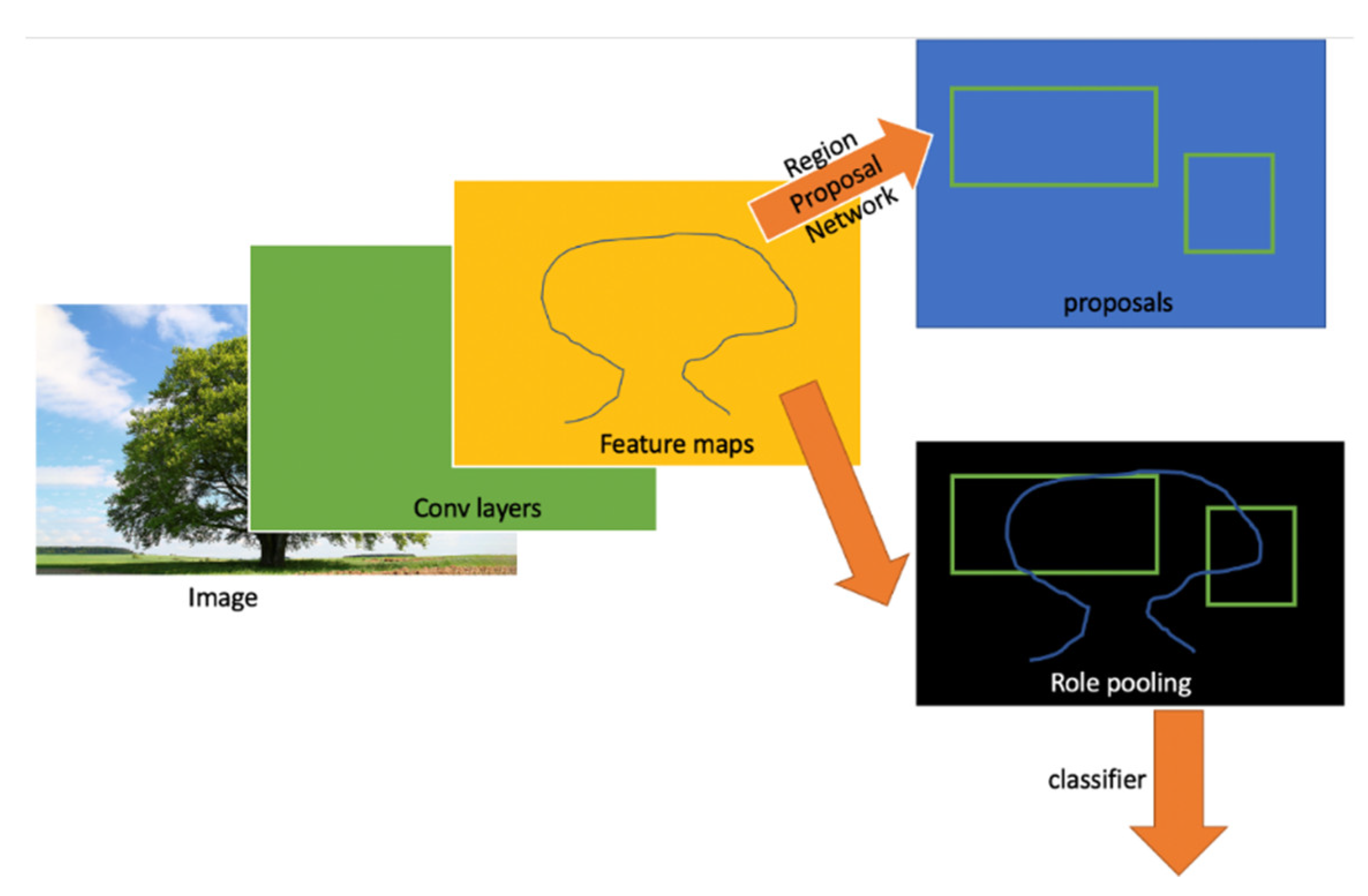
2.2.4. Faster R-CNN
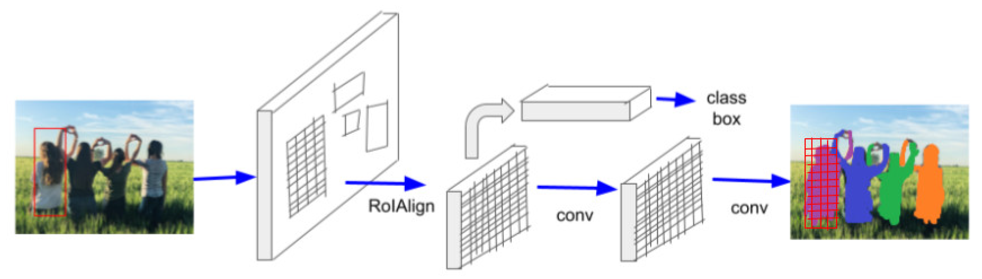
2.2.5. Mask R-CNN
2.2.6. You Only Look Once (YOLO)
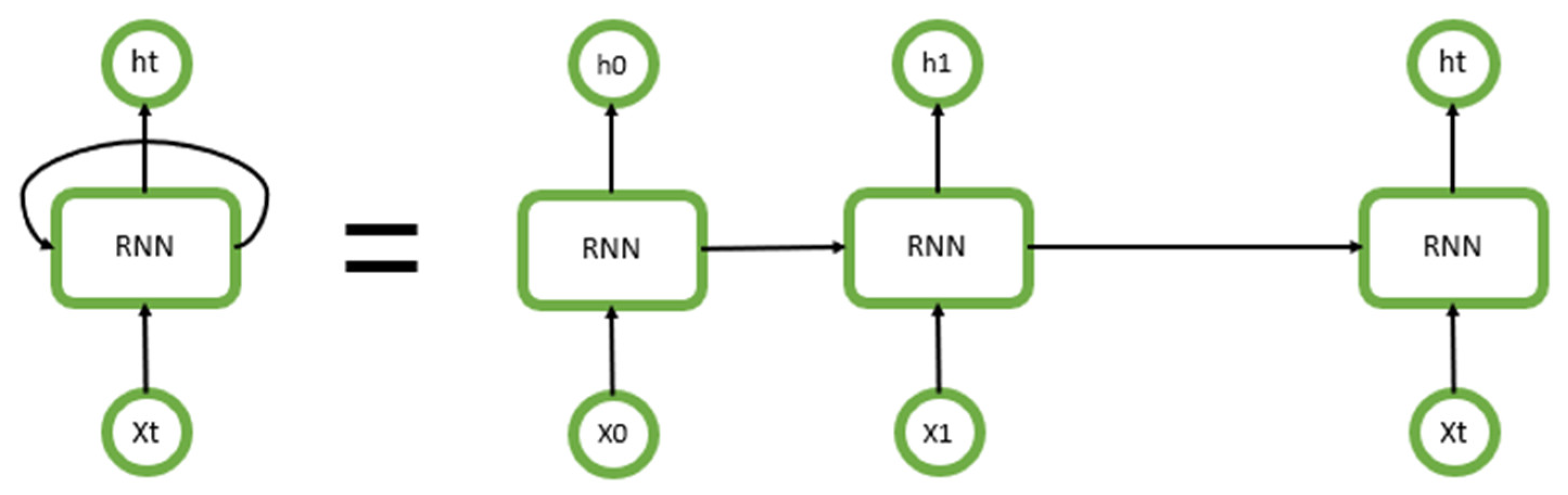
2.2.7. RNN
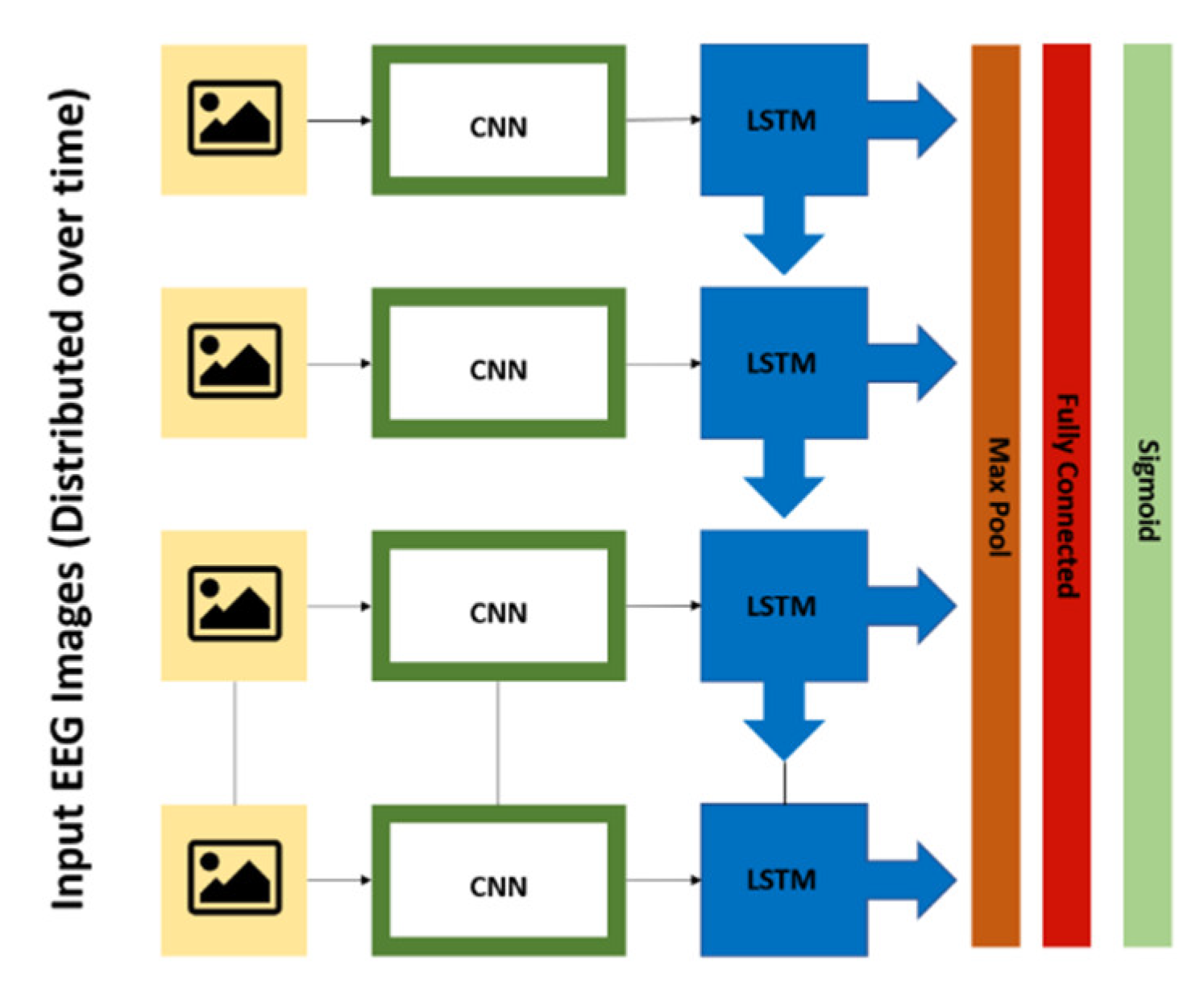
2.2.8. CRNN
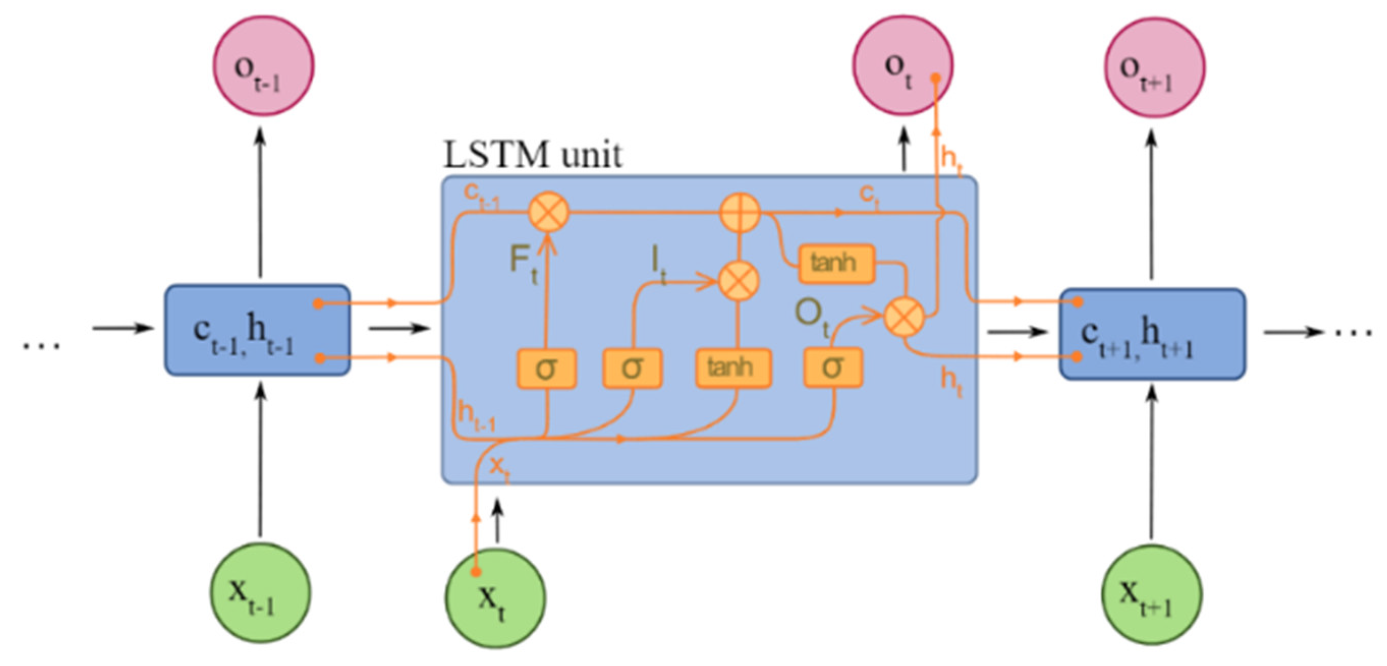
2.2.9. LSTM
2.2.10. GAN
2.3. Distributed System (DS)
- Concurrency: Each node can perform different tasks or parts of the same task-sharing resources, allowing parallel computing.
- Quality of service: this concept refers to the idea that a specific type of message’s sensibility depends on the type of information transmitted. For example, if you download a file, it may not be vital if it delays for some seconds. However, in a phone call, or a video call, any delay may result in a loss of data that troubles communication.
- Scalability: Any network must be built, having in mind that it may expand.
- Security: With the constant growth of devices connected to the cloud, and the high amount of information transmitted, safety must be implemented on every network designed.
- Failure handling: In a DS, there must be a plan for possible failures. If a computer fails, the others will keep working.
- No global clock: This happens because of the communication through messages. Each node may have its frequency of operation as each one has its own hardware. This situation may difficult the transmission because there is a limit to computer synchronization accuracy in a network. Therefore, a bottleneck in communication, where the best bandwidth that may be reached is the lowest in the network, may be caused. This allows each node to operate independently with its requirements of hardware.
2.4. Metrics for Evaluation
2.5. Frenét Motion Planning
3. Methods to Address the Pipeline of End-To-End ADS
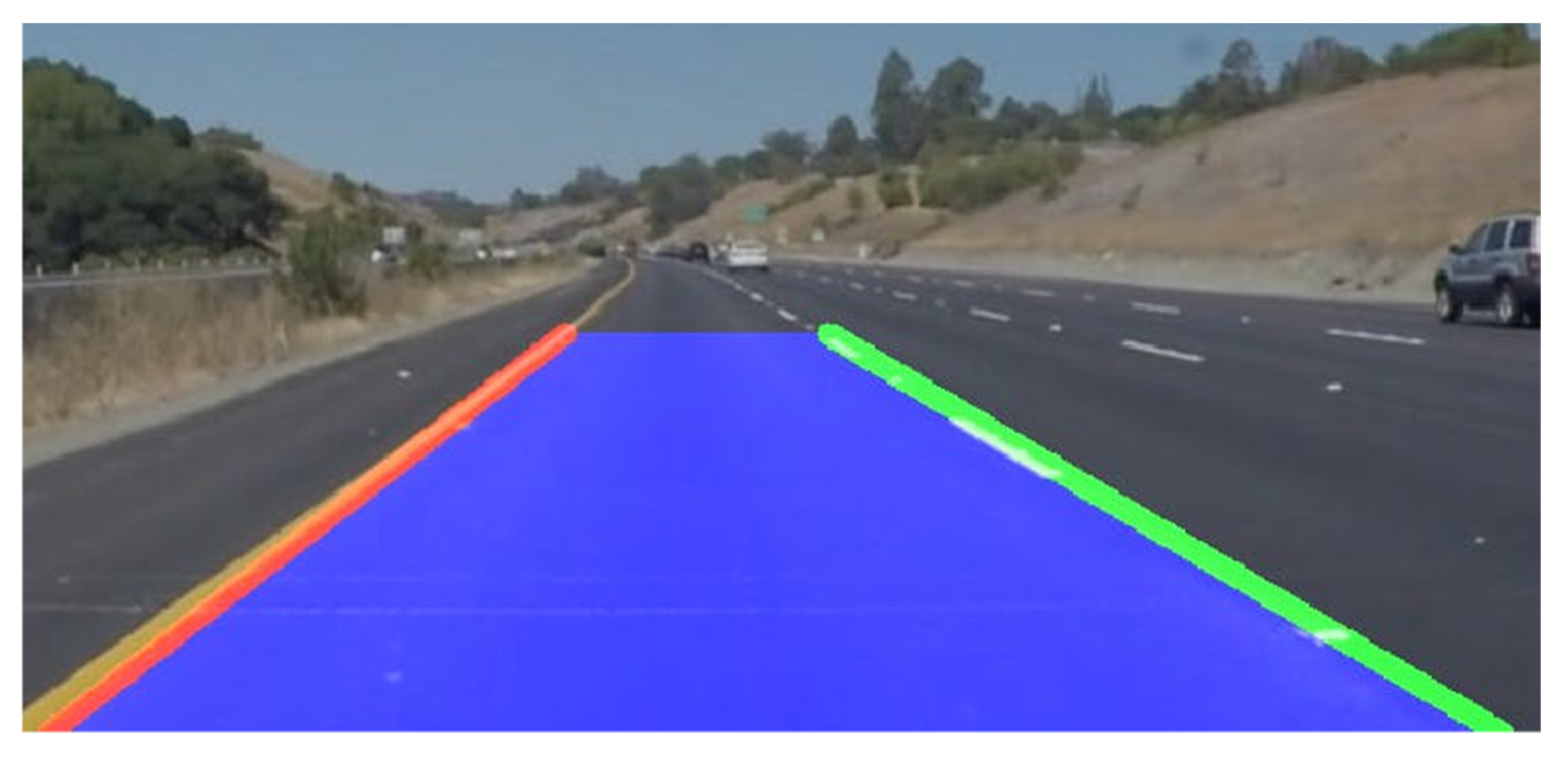
3.1. Image Pre-Processing and Instance Segmentation
3.2. Driver Assistance and Predicting Driver Patterns
3.2.1. Behavioral Cloning (BC)
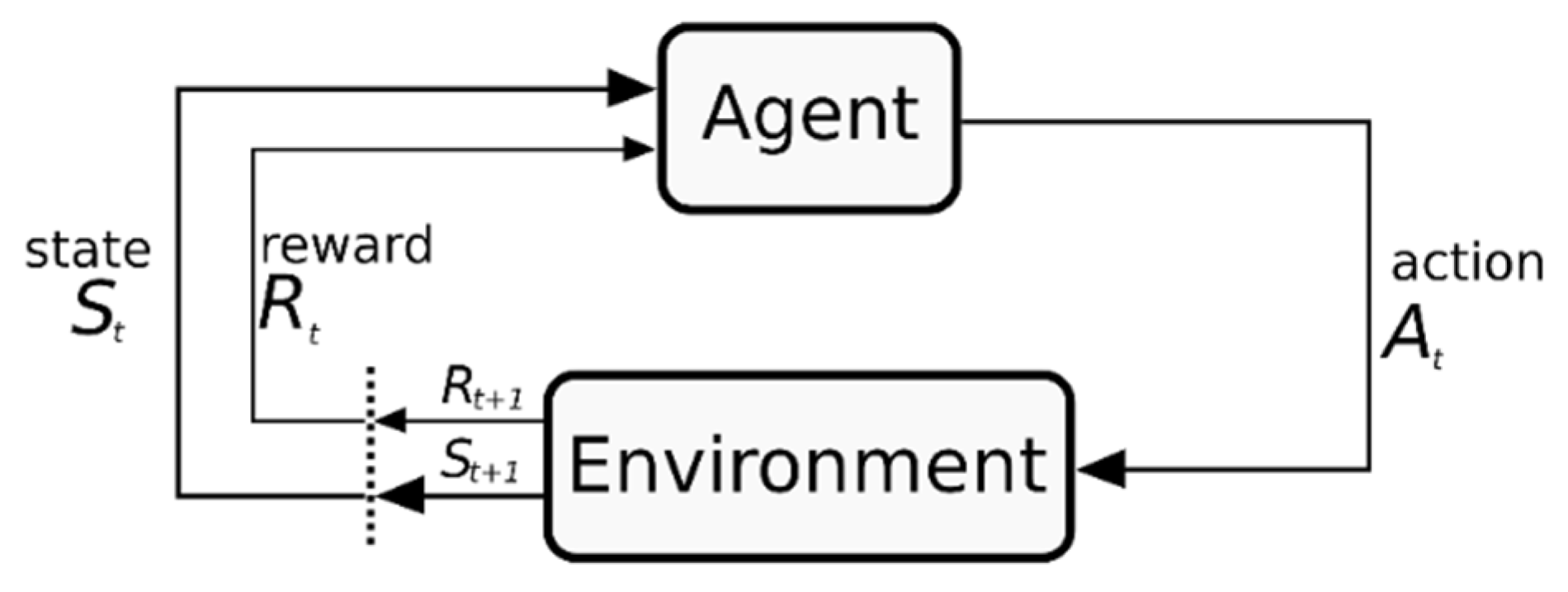
3.2.2. Reinforcement Learning (RL)
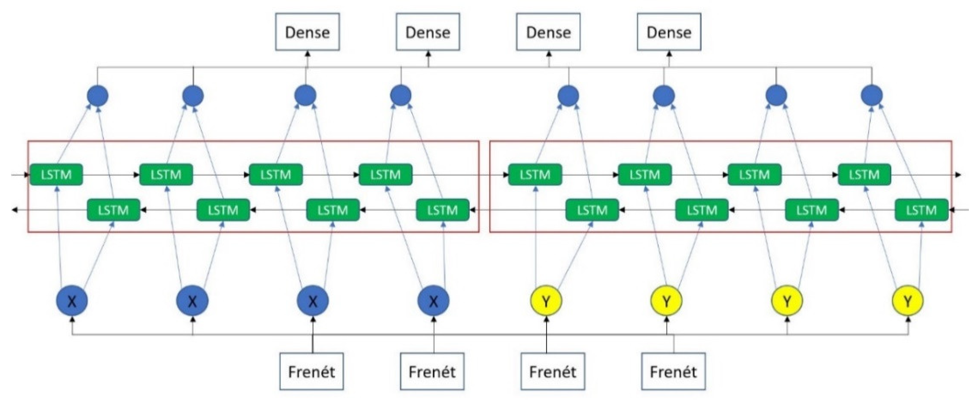
3.2.3. LSTM Based Models
3.3. Human Sentiment Analysis
3.4. Using the Cloud with Autonomous Driving Systems
4. Future Trends
4.1. Cloud Computing
- Data is gathered on an edge. In this case, an AV or a group of AVs can be considered an extreme edge.
- There is a lot of data being generated in a large geographic area.
- The information gathered needs to be analyzed, and it has to provoke a response in less than a second.
4.2. Parallelization of Neural Networks
- Data parallelism: Data parallelism is a different kind of parallelism that, instead of relying on the process or task concurrency, is related to both the flow and the information structure. Each GPU uses the same model to trains on different data subsets. If there are too many computational nodes, it is necessary to reduce the learning rate to keep a smooth training process.
- Model parallelism: In model parallelism, each computational node is responsible for parts of the model by training the same data samples. The computational nodes communicate between them when a neuron’s input is from another computational node’s output. However, the performance is worse than data parallelism, and the performance of the network will be decreased if it has too many nodes.
- Data-model parallelism: Both previous models have disadvantages, but they also have positive characteristics. Model parallelism could get good performance with many neuron activities, and data parallelism is efficient with many weights.
4.3. Parallelization of the Whole System
4.4. First Thoughts towards an Approach for LSTM-Based Path Planning Prediction
5. Conclusions
Author Contributions
Funding
Acknowledgments
Conflicts of Interest
Abbreviations
| ADS | Autonomous Driving System |
| AV | Autonomous Vehicle |
| AP | Average Precision |
| mAP | Mean Average Precision |
| BC | Behavioral Cloning |
| BEV | Bird’s Eye View |
| CDBN | Convolutional Deep Belief Network |
| CLDA | Constrained Linear Discriminant Analysis |
| CNN | Convolutional Neural Network |
| COCO-ODC | Common Objects in Context Object Detection Challenge |
| CRNN | Convolutional Recurrent Neural Network |
| CUDA | Compute Unified Device Architecture |
| DAG-SVM | Directed Acyclic Graph-Support Vector Machine |
| DARPA | Defense Advanced Research Projects Agency |
| DBN | Deep Belief Network |
| DDNN | Distributed Deep Neural Network |
| DS | Distributed System |
| DOG | Difference of Gaussian |
| FCN | Fully Convolutional Network |
| FP | False Positive |
| FN | False Negative |
| GAN | Generative Adversarial Network |
| IARA | Intelligent Autonomous Robotics Automobile |
| IDM | Intelligent Driver Model |
| IoU | Intersection over Union |
| LiDAR | Light Detection and Ranging |
| LSTM | Long Short-Term Memory |
| MOT | Multi-Object Tracking |
| M3OT | 3D Multi-Object Tracking |
| MV3D | Multi-View 3D Object Detection Network for Autonomous Driving |
| MVX-Net | Multimodal Voxel for 3D Object Detection Network |
| NHTSA | National Highway Traffic Safety Administration |
| NN | Neural Network |
| R-CNN | Region-Based Convolutional Neural Network |
| RL | Reinforcement Learning |
| RNN | Recurrent Neural Network |
| RPN | Region Proposal Network |
| RoI | Region of Interest |
| SAE | Society of Autonomous Engineers |
| SIFT | Scale Invariant Feature TransformScale Invariant Feature Transform |
| SLAM | Simulation Localization And Mapping |
| SURF | Speeded-Up Robust Features |
| TN | True Negative |
| TP | True Positive |
| VOC | Visual Object Classes |
| YOLO | You Only Look Once |
References
- Singh, S. Critical Reasons for Crashes Investigated in the National Motor Vehicle Crash Causation Survey; National Highway Traffic Safety Administration; U.S. Department of Transportation, National Highway Traffic Safety Administration: Washington, DC, USA, 2015.
- Rangesh, A.; Trivedi, M.M. No Blind Spots: Full-Surround Multi-Object Tracking for Autonomous Vehicles Using Cameras and LiDARs. IEEE Trans. Intell. Veh. 2019, 4, 588–599. [Google Scholar] [CrossRef]
- Huang, Y.; Chen, Y. Autonomous Driving with Deep Learning: A Survey of State-of-art Technologies. arXiv 2020, arXiv:2006.06091. [Google Scholar]
- Yurtsever, E.; Lambert, J.; Carballo, A.; Takeda, K. A Survey of Autonomous Driving: Common Practices and Emerging Technologies. IEEE Access 2020, 8, 58443–58469. [Google Scholar] [CrossRef]
- Badue, C.; Guidolini, R.; Vivacqua, R.; Azevedo, P.; Brito, V.; Forechi, A.; Ferreira, A. Self-Driving Cars: A Survey. arXiv 2019, arXiv:1901.04407. [Google Scholar] [CrossRef]
- Szymak, P.; Piskur, P.; Naus, K. The Effectiveness of Using a Pretrained Deep Learning Neural Networks for Object Classification in Underwater Video. Remote. Sens. 2020, 12, 3020. [Google Scholar] [CrossRef]
- Lowe, D.G. Object recognition from local scale-invariant features. In Proceedings of the International Conference on Computer Vision, Corfu, Greece, 20–25 September 1999; pp. 1150–1157. [Google Scholar]
- Bay, H.; Ess, A.; Tuytelaars, T.; Van Gool, L. Speeded Up Robust Features. Comput. Vis. Image Underst. 2008, 110, 346–359. [Google Scholar] [CrossRef]
- Cortes Gallardo-Medina, E.; Moreno-Garcia, C.F.; Zhu, A.; Chípuli-Silva, D.; González-González, J.A.; Morales-Ortiz, D.; Fernández, S.; Urriza, B.; Valverde-López, J.; Marín, A.; et al. A Comparison of Feature Extractors for Panorama Stitching in an Autonomous Car Architecture. In Proceedings of the IEEE International Conference on Mechatronics, Electronics and Automotive Engineering (ICMEAE), Cuernavaca, Mexico, 26–29 November 2019. [Google Scholar]
- Varghese, J.Z.; Boone, R.G. Overview of Autonomous Vehicle Sensors and Systems. In Proceedings of the International Conference on Operations Excellence and Service Engineering, Orlando, FL, USA, 10–11 September 2015. [Google Scholar]
- Beltran, J.; Guindel, C.; Moreno, F.M.; Cruzado, D.; Garcia, F.; De La Escalera, A. BirdNet: A 3D Object Detection Framework from LiDAR Information. In Proceedings of the IEEE International Conference on Intelligent Transportation Systems, Maui, HI, USA, 4–7 November 2018. [Google Scholar]
- Chen, X.; Ma, H.; Wan, J.; Li, B.; Xia, T. Multi-View 3D Object Detection Network for Autonomous Driving. In Proceedings of the IEEE Conference on Computer Vision and Pattern Recognition (CVPR), Honolulu, HI, USA, 21–26 July 2017. [Google Scholar]
- Geiger, A.; Moosmann, F.; Car, O.; Schuster, B. A Toolbox for Automatic Calibration of Range and Camera Sensors Using a Single Shot. In Proceedings of the IEEE International Conference on Robotics and Automation (ICRA), Saint Paul, MN, USA, 14–18 May 2012; pp. 3936–3943. [Google Scholar]
- Vora, S.; Lang, A.H.; Helou, B.; Beijbom, O. PointPainting: Sequential Fusion for 3D Object Detection. arXiv 2019, arXiv:1911.10150. [Google Scholar]
- Starr, W.; Lattimer, B.Y. A Comparison of IR Stereo Vision and LiDAR for Use in Fire Environments. In Proceedings of the Sensors, 2012 IEEE, Taipei, Taiwan, 28–31 October 2012. [Google Scholar]
- Viitaniemi, V.; Laaksonen, J. Techniques for Image Classification, Object Detection and Object Segmentation. Visual Information Systems. Web-Based Visual Information Search and Management, Lecture Notes in Computer Science. In Proceedings of the VISUAL 2008, Salerno, Italy, 11–12 September 2008; Springer: Berlin/Heidelberg, Germany, 2008; Volume 5188. [Google Scholar]
- Leonard, J.K. Image Classification and Object Detection Algorithm Based on Convolutional Neural Network. Sci. Insights 2019, 31, 85–100. [Google Scholar] [CrossRef]
- Chen, C.; Qin, C.; Qiu, H.; Tarroni, G.; Duan, J.; Bai, W.; Rueckert, D. Deep Learning for Cardiac Image Segmentation: A Review. Front. Cardiovasc. Med. 2020, 7, 25. [Google Scholar] [CrossRef]
- Tabian, I.; Fu, H.; Khodaei, Z.S. A Convolutional Neural Network for Impact Detection and Characterization of Complex Composite Structures. Sensors 2019, 19, 4933. [Google Scholar] [CrossRef] [PubMed]
- Sabzekar, M.; Ghasemigol, M.; Naghibzadeh, M.; Yazdi, H.S. Improved DAG-SVM: A New Method for Multiclass SVM Classification; ICAI: Las Vegas, NV, USA, 2012. [Google Scholar]
- Du, Q. Unsupervised Real-Time Constrained Linear Discriminate Analysis to Hyper Spectral Image Classification. Pattern Recognit. 2007, 40, 1510–1519. [Google Scholar] [CrossRef]
- Lecun, Y.; Bottou, L.; Bengio, Y. Gradient-based Learning Applied to Document Recognition. Proc. IEEE 1998, 86, 2278–2324. [Google Scholar] [CrossRef]
- Lee, H.; Grosse, R.; Ranganath, R.; Ng, A.Y. Convolutional Deep Belief Networks for Scalable Unsupervised Learning of Hierarchical Representations. In Proceedings of the 26th Annual International Conference on Machine Learning, Montreal, QC, Canada, 14–18 June 2009; pp. 609–616. [Google Scholar]
- Girshick, R.; Donahue, J.; Darrell, T.; Malik, J. Rich Feature Hierarchies for Accurate Object Detection and Semantic Segmentation. In Proceedings of the IEEE Conference on Computer Vision and Pattern Recognition, Columbus, OH, USA, 23–28 June 2014; pp. 580–587. [Google Scholar]
- He, K.; Gkioxari, G.; Dollar, P.; Girshick, R. Mask R-CNN. Facebook AI Res. 2018, 1–12. [Google Scholar]
- Redmon, J.; Divvala, S.; Girshick, R.; Farhadi, A. You Only Look Once: Unified, Real-Time Object Detection. arXiv 2015, arXiv:1506.02640. [Google Scholar]
- Simonyan, J.K.; Zisserman, A. Very Deep Convolutional Networks for Large-Scale Image Recognition. In Proceedings of the International Conference on Learning Representations, San Diego, CA, USA, 7–9 May 2015. [Google Scholar]
- Pascanu, R.; Mikolov, T.; Bengio, Y. On the Difficulty of Training Recurrent Neural Networks. arXiv 2012, arXiv:1211.5063. [Google Scholar]
- Choi, K.; Fazekas, G.; Sandler, M.; Cho, K. Convolutional Recurrent Neural Networks for Music Classification. In Proceedings of the IEEE International Conference on Acoustics, Speech and Signal Processing (ICASSP), New Orleans, LA, USA, 5–9 March 2017; pp. 2392–2396. [Google Scholar]
- Çakır, E.; Parascandolo, G.; Heittola, T.; Huttunen, H.; Virtanen, T. Convolutional Recurrent Neural Networks for Polyphonic Sound Event Detection. IEEE/ACM Trans. Audio Speech Lang. Process. 2017, 25, 1291–1303. [Google Scholar] [CrossRef]
- Maddula, R.; Stivers, J.; Mousavi, M.; Ravindran, S.; Sa, V.D. Deep Recurrent Convolutional Neural Networks for Classifying P300 BCI signals. In Proceedings of the 7th Graz Brain-Computer Interface Conference, Graz, Austria, 18–22 September 2017. [Google Scholar]
- Zuo, Z.; Shuai, B.; Wang, G.; Liu, X.; Wang, X.; Wang, B.; Chen, Y. Convolutional Recurrent Neural Networks: Learning Spatial Dependencies for Image Representation. In Proceedings of the IEEE Conference on Computer Vision and Pattern Recognition, Boston, MA, USA, 7–12 June 2015; pp. 18–26. [Google Scholar]
- Hu, Z.; Hu, Y.; Liu, J.; Wu, B.; Han, D.; Kurfess, T. A CRNN module for hand pose estimation. Neurocomputing 2019, 333, 157–168. [Google Scholar] [CrossRef]
- Hochreiter, S.; Schmidhuber, J. Long Short-Term Memory. Neural Comput. 1997, 9, 1735–1780. [Google Scholar] [CrossRef] [PubMed]
- Goodfellow, I.; Pouget-Abadie, J.; Mirza, M.; Xu, B.; Warde-Farley, D.; Ozair, S.; Courville, A.; Bengio, Y. Generative Adversarial Nets. In Proceedings of the Advances in Neural Information Processing Systems, Montreal, QC, Canada, 8–13 December 2014. [Google Scholar]
- Mirza, M.; Osindero, S. Conditional Generative Adversarial Nets. arXiv 2014, arXiv:1411.1784. [Google Scholar]
- Odena, A. Semi-supervised Learning with Generative Adversarial Networks. arXiv 2016, arXiv:1606.01583. [Google Scholar]
- Odena, A.; Olah, C.; Shlens, J. Conditional Image Synthesis with Auxiliary Classifier GANs. In Proceedings of the International Conference on Machine Learning, Sydney, Australia, 6–11 August 2017. [Google Scholar]
- Ali-Gombe, A.; Elyan, E.; Savoye, Y.; Jayne, C. Few-shot classifier GAN. In Proceedings of the International Joint Conference on Neural Networks (IJCNN), Rio de Janeiro, Brazil, 8–13 July 2018. [Google Scholar]
- Yong, F.; Tanfeng, S.; Xinghao, J.; Ke, X.; Paisong, H. Robust GAN-Face Detection Based on Dual-Channel CNN Network. In Proceedings of the 12th International Congress on Image and Signal Processing, BioMedical Engineering and Informatics (CISP-BMEI), Suzhou, China, 19–21 October 2018; pp. 1–5. [Google Scholar]
- Ali-Gombe, A.; Elyan, E.; Jayne, C. Fish Classification in Context of Noisy Images. Eng. Appl. Neural Netw. 2017, CCIS 744, 216–226. [Google Scholar]
- Elyan, E.; Jamieson, L.; Ali-Gombe, A. Deep learning for symbols detection and classification in engineering drawings. Neural Networks 2020, 129, 91–102. [Google Scholar] [CrossRef]
- Coulouris, G.; Dollimore, J.; Kindberg, T.; Blair, G. Distributed Systems Concepts and Design; Addison-Wesley: Boston, MA, USA, 2012. [Google Scholar]
- Usman, M.; Anjum, A.; Farid, M.; Antonpoulos, N. Cloud-Based Video Analytics Using Convolutional Neural Networks. Softw. Pract. Exp. 2019, 49, 565–583. [Google Scholar]
- Teerapittayanon, S.; McDanel, B.; Kung, H.T. Distributed Deep Neural Networks over the Cloud, the Edge and End Devices. In Proceedings of the 2017 IEEE 37th International Conference on Distributed Computing Systems (ICDCS), Atlanta, GA, USA, 5–8 June 2017. [Google Scholar]
- Khandelwa, R. COCO and Pascal VOC Data Format for Object Detection. Towards Data Science. Available online: https://towardsdatascience.com/coco-data-format-for-object-detection-a4c5eaf518c5 (accessed on 17 October 2020).
- Zeng, N. An Introduction to Evaluation Metrics for Object Detection. Available online: https://blog.zenggyu.com/en/post/2018-12-16/an-introduction-to-evaluation-metrics-for-object-detection/ (accessed on 17 October 2020).
- El Aidouni, M. Evaluating Object Detection Models: Guide to Performance Metrics. Available online: https://manalelaidouni.github.io/manalelaidouni.github.io/Evaluating-Object-Detection-Models-Guide-to-Performance-Metrics.html (accessed on 17 October 2020).
- Werling, M.; Ziegler, J.; Kammel, S.; Thrun, S. Optimal Trajectory Generation for Dynamic Street Scenarios in a Frenét Frame. In Proceedings of the 2010 IEEE International Conference on Robotics and Automation, Anchorage, AK, USA, 3–7 May 2010. [Google Scholar]
- Zhou, Y.; Tuzel, O. VoxelNet End-to-End Learning for Point Cloud Based 3D Object Detection. arXiv 2017, arXiv:1711.06396. [Google Scholar]
- Zhou, Y.; Tuzel, O. MVX-Net: Multimodal VoxelNet for 3D Object Detection. In Proceedings of the 2019 International Conference on Robotics and Automation (ICRA), Montreal, QC, Canada, 20–24 May 2019. [Google Scholar]
- Liu, T.; Liao, Q.; Gan, L.; Ma, F.; Cheng, J.; Xie, X.; Wang, Z.; Chen, Y.; Zhu, Y.; Zhang, S.; et al. Hercules: An Autonomous Logistic Vehicle for Contact-less Goods Transportation During the Covid-19 Outbreak. arXiv 2020, arXiv:2004.07480. [Google Scholar]
- Moraes, G.; Mozart, A.; Azevedo, P.; Piumbini, M.; Cardoso, V.B.; Oliveira-Santos, T.; De Souza, A.F.; Badue, C. Image-Based Real-Time Path Generation Using Deep Neural Networks. In Proceedings of the 2020 International Joint Conference on Neural Networks (IJCNN), Glasgow, UK, 19–24 July 2020. [Google Scholar]
- Cardoso, V.B.; Oliveira, A.S.; Forechi, A.; Azevedo, P.; Mutz, F.; Oliveira-Santos, T.; Badue, C.; De Souza, A.F. A Large-Scale Mapping Method Based on Deep Neural Networks Applied to Self-Driving Car Localization. In Proceedings of the 2020 International Joint Conference on Neural Networks (IJCNN), Glasgow, UK, 19–24 July 2020. [Google Scholar]
- Weaver, C. Self-Driving Cars Learn to Read the Body Language of People on the Street, IEEE SPECTRUM. Available online: https://spectrum.ieee.org/transportation/self-driving/selfdriving-cars-learn-to-read-the-body-language-of-people-on-the-street (accessed on 17 October 2020).
- Aranzeta-Ojeda, L.; Moreno-García, C.F.; Granados-Reyes, A.; Bustamante-Bello, R. Design, Development and Testing of a Low-Cost, High Sensitivity System for Neurodegenerative Disease Detection and Characterization. In Proceedings of the International Conference on Microtechnologies and Medical Biology (MMB), Lucerne, Switzerland, 4–6 May 2011; pp. 64–65. [Google Scholar]
- Bustamante-Bello, R.; Aranzeta-Ojeda, L.; Moreno-Garcia, C.F. Design and Development of a Low-Cost, High Sensitivity Device for Neurodegenerative Disease Detection. In Proceedings of the 24th IEEE International Conference Micro Electro Mechanical Systems (MEMS), Cancun, Mexico, 23–27 January 2011. [Google Scholar]
- Barea, R.; Bergasa, L.M.; Romera, E.; López-Guillén, E.; Perez, O.; Tradacete, M.; López, J. Integrating State-of-the-Art CNNs for Multi-Sensor 3D Vehicle Detection in Real Autonomous Driving Environments. In Proceedings of the IEEE Intelligent Transportation Systems Conference (ITSC), Auckland, New Zealand, 27–30 October 2019; Volume 1. [Google Scholar]
- Shah, N.; Shankar, A.; Park, J.-h. Detecting Drivable Area for Autonomous Vehicles. arXiv 2020, arXiv:1911.02740. [Google Scholar]
- Meng, X.; Lee, K.K.; Xu, Y. Human Driving Behavior Recognition Based on Hidden Markov Models. In Proceedings of the 2006 IEEE International Conference on Robotics and Biomimetics, Kunming, China, 17–20 December 2006. [Google Scholar]
- Curiel-Ramirez, L.A.; Ramirez-Mendoza, R.A.; Bautista-Montesano, R.; Bustamante-Bello, M.R.; Gonzalez-Hernandez, H.G.; Reyes-Avedaño, J.A.; Gallardo-Medina, E.C. End-to-End Automated Guided Modular Vehicle. Appl. Sci. 2020, 10, 4400. [Google Scholar] [CrossRef]
- Sutton, R.S.; Barto, A.G. Reinforcement Learning: An Introduction, 2nd ed.; The MIT Press: Cambridge, MA, USA, 2018. [Google Scholar]
- Hoel, C.J.; Wolff, K.; Laine, L. Automated Speed and Lane Change Decision Making using Deep Reinforcement Learning. In Proceedings of the 2018 21st International Conference on Intelligent Transportation Systems (ITSC), Maui, HI, USA, 4–7 November 2018. [Google Scholar]
- El Sallab, A.; Abdou, M.; Perot, E.; Yogamani, S. Deep Reinforcement Learning framework for Autonomous Driving. Electron. Imaging 2017, 2017, 70–76. [Google Scholar] [CrossRef]
- Bai, Z.; Cai, B. Deep Learning-Based Motion Planning for Autonomous Vehicle Using Spatiotemporal LSTM Network. arXiv 2019, arXiv:1903.01712. [Google Scholar]
- Atlché, F.; de la Fortelle, A. An LSTM Network for Highway Trajectory Prediction. arXiv 2018, arXiv:1801.07962. [Google Scholar]
- Yan, S.; Teng, Y.; Smith, J.; Zhang, B. Driver behavior recognition based on deep convolutional neural networks. In Proceedings of the 12th International Conference on Natural Computation, Fuzzy Systems and Knowledge Discovery (ICNC-FSKD), Changsha, China, 13–15 August 2016; pp. 636–641. [Google Scholar]
- Naqvi, R.A.; Arsalan, M.; Rehman, A.; Rehman, A.U.; Loh, W.-K.; Paul, A. Deep Learning-Based Drivers Emotion Classification System in Time Series Data for Remote Applications. Remote. Sens. 2020, 12, 587. [Google Scholar] [CrossRef]
- Hu, Y.; Lu, M.; Lu, X. Feature refinement for image-based driver action recognition via multi-scale attention convolutional neural network. Signal Process. Image Commun. 2020, 81, 115697. [Google Scholar] [CrossRef]
- Kim, C.-M.; Hong, E.J.; Chung, K.; Park, R.C. Driver Facial Expression Analysis Using LFA-CRNN-Based Feature Extraction for Health-Risk Decisions. Appl. Sci. 2020, 10, 2956. [Google Scholar] [CrossRef]
- Liu, S.; Tang, J.; Wang, C.; Wang, Q.; Gaudiot, J.L. Implementing a Cloud Platform for Autonomous Driving. arXiv 2017, arXiv:1704.02696. [Google Scholar]
- Kumar, S.; Gollakota, S.; Katabi, D. A Cloud-Assisted Design for Autonomous Driving. In Proceedings of the First Edition of the MCC Workshop on Mobile Cloud Computing (MCC); ACM: Helsinki, Finland, 2012. [Google Scholar]
- Li, X.; Zhang, G.; Li, K.; Wang, Z. Chapter 4: Deep Learning and Its Parallelization. In Big Data: Principles and Paradigms; Morgan Kauffman: Burlington, MA, USA, 2016. [Google Scholar]


Publisher’s Note: MDPI stays neutral with regard to jurisdictional claims in published maps and institutional affiliations. |
© 2021 by the authors. Licensee MDPI, Basel, Switzerland. This article is an open access article distributed under the terms and conditions of the Creative Commons Attribution (CC BY) license (http://creativecommons.org/licenses/by/4.0/).
Share and Cite
Cortés Gallardo Medina, E.; Velazquez Espitia, V.M.; Chípuli Silva, D.; Fernández Ruiz de las Cuevas, S.; Palacios Hirata, M.; Zhu Chen, A.; González González, J.Á.; Bustamante-Bello, R.; Moreno-García, C.F. Object Detection, Distributed Cloud Computing and Parallelization Techniques for Autonomous Driving Systems. Appl. Sci. 2021, 11, 2925. https://doi.org/10.3390/app11072925
Cortés Gallardo Medina E, Velazquez Espitia VM, Chípuli Silva D, Fernández Ruiz de las Cuevas S, Palacios Hirata M, Zhu Chen A, González González JÁ, Bustamante-Bello R, Moreno-García CF. Object Detection, Distributed Cloud Computing and Parallelization Techniques for Autonomous Driving Systems. Applied Sciences. 2021; 11(7):2925. https://doi.org/10.3390/app11072925
Chicago/Turabian StyleCortés Gallardo Medina, Edgar, Victor Miguel Velazquez Espitia, Daniela Chípuli Silva, Sebastián Fernández Ruiz de las Cuevas, Marco Palacios Hirata, Alfredo Zhu Chen, José Ángel González González, Rogelio Bustamante-Bello, and Carlos Francisco Moreno-García. 2021. "Object Detection, Distributed Cloud Computing and Parallelization Techniques for Autonomous Driving Systems" Applied Sciences 11, no. 7: 2925. https://doi.org/10.3390/app11072925
APA StyleCortés Gallardo Medina, E., Velazquez Espitia, V. M., Chípuli Silva, D., Fernández Ruiz de las Cuevas, S., Palacios Hirata, M., Zhu Chen, A., González González, J. Á., Bustamante-Bello, R., & Moreno-García, C. F. (2021). Object Detection, Distributed Cloud Computing and Parallelization Techniques for Autonomous Driving Systems. Applied Sciences, 11(7), 2925. https://doi.org/10.3390/app11072925