Abstract
With the combustion of solid fuels, emissions such as particulate matter are also formed, which have a negative impact on human health. Reducing their amount in the air can be achieved by optimizing the combustion process as well as the flue gas flow. This article aims to optimize the flue gas tract using separation baffles. This design can make it possible to capture particulate matter by using three baffles and prevent it from escaping into the air in the flue gas. The geometric parameters of the first baffle were changed twice more. The dependence of the flue gas flow on the baffles was first observed by computational fluid dynamics (CFD) simulations and subsequently verified by the particle imaging velocimetry (PIV) method. Based on the CFD results, the most effective is setting 1 with the same boundary conditions as those during experimental PIV measurements. Setting 2 can capture 1.8% less particles and setting 3 can capture 0.6% less particles than setting 1. Based on the stoichiometric calculations, it would be possible to capture up to 62.3% of the particles in setting 1. The velocities comparison obtained from CFD and PIV confirmed the supposed character of the turbulent flow with vortexes appearing in the flue gas tract, despite some inaccuracies.
1. Introduction
Human health depends on air quality. Emissions, especially particulate matter (PM), contained in the air can penetrate the lungs and blood circulation, which can cause various respiratory and cardiovascular diseases [1,2]. Therefore, it is important to search for possibilities to reduce the concentration of PM in the air. The air pollution with particulate matter is mainly caused by traffic, industrial activity, domestic fuel combustion, natural sources, and unspecified sources of human origin [3,4]. The largest producer of particulate matter in Central Europe, where Slovakia is also located, is domestic fuel combustion [4], which is also the interest of this article.
There are also the air quality standards for particulate matter based on the European Union (EU) limits and the air quality guidelines (AQG) set by the World Health Organization (WHO). The limit values for particulate matter with a diameter of 10 μm or less (PM10) are as follows: (I) 50 μm/m3 per 1 day given by the EU limit value and also the WHO AQG, (II) 40 μm/m3 per calendar year given by the limit value, and (III) 20 μm/m3 per calendar year given by the WHO WQG. The limit values for particulate matter with a diameter of 2.5 μm or less (PM2.5) are as follows: (I) 25 μm/m3 per 1 day given only by the WHO AQG, (II) 25 μm/m3 per calendar year given by the EU limit value, and (III) 10 μm/m3 per calendar year given by the WHO WQG [5].
It is important to capture these particles before they escape into the air. With this aim, there is an effort to optimize the combustion process, and also various geometric constructions can be proposed, which are inserted into the heat sources. Their installation and maintenance are easier compared to other types of separators placed into the chimney. The produced fly ash from combustion can also be used for making nanoporous materials, e.g., for capturing carbon dioxide (CO2), as is stated in the work of Miricioiu and Niculescu [6].
The optimization of a biomass boiler by an air manifold was investigated by Bianco et al. The authors found out that reducing the entropy meant improving the device performances [7]. The research of Smith et al. was focused on the optimization of biomass combustion by burner designs [8]. The main interest of the work of Nussbaumer et al. was the secondary air injection with the aim of the optimization of fluid dynamics for combustion improvement [9]. Athanasios et al. investigated an optimized wood boiler manufactured by a Greek company, which should belong in Class 3 of the EN303-5 standard [10]. All these works chose the approach of using CFD simulations, some of which were verified experimentally or, in the case of Nussbaumer et al., using the PIV method. However, none of these works dealt with optimization aimed at capturing particulate matter. Therefore, there is little knowledge regarding particulate matter tracking in the combustion chamber or flue gas tract of the heat source.
In the cases of combustion simulation, realizable k−ε models are used, where k is the turbulence kinetic energy and ε is the dissipation rate of the turbulence kinetic energy. This approach was also chosen by Bianco et al., where it was stated that the advantage of the realizable k−ε model is the modified dissipation rate equation and damping function [7]. A realizable k-ε model was also used by Silva et al. in their research of industrial furnaces. The authors showed results of fields for temperature, velocity, and concentration of carbon monoxide (CO) and carbon dioxide (CO2), which should be a tool for the optimization [11]. In the research of Gómez et al., turbulence was modeled by a realizable k–ε model. They simulated a biomass boiler and analyzed the thermal behavior using exhaust gas recirculation [12]. A realizable k−ε model with enhanced wall functions was chosen in the work of Zadravec et al. They investigated air staged combustion, which led to lower emissions and higher thermal efficiency [13]. The standard k−ε model was used in the works of Smith et al. and Athanasios et al.
Measurements of particle velocity can be performed using particle imaging velocimetry (PIV). The laser light sheet illuminates the observed flow, and the instantaneous figures are captured. The figure analysis allows obtaining flow fields [14]. This method has been used for the observation of the flue gas velocity during solid fuel combustion in several works. Mizeraczyk et al. investigated the velocity field in an electrostatic precipitator by using the PIV method. Their work showed the importance of the secondary flows, which influenced the motion and precipitation of small particles [15]. The flow field of the pulverized coal flame was observed by the PIV method in the work of Sung and Choi. They focused on the heat release region and the internal recirculation zone [16]. The combined approach of PIV and particle tracking velocimetry (PTV) was used by Schneider et al. in their work. They also investigated the flow field of solid fuel particles in the combustion chamber [17]. However, most of the works were focused on the observation of velocity in areas outside the flue gas tract.
Based on this knowledge, it is important to search for possibilities to decrease the particulate matter in the environment. One of the possibilities can be capturing particulate matter in the flue gas tract caused by geometric modification of the heat source, which is also the aim of this article. For this case, a wood stove modified by three baffles placed in the flue gas tract was chosen. The effect of baffles was observed using CFD simulation, while geometric parameters of the first baffle were changed, and was verified using the PIV method. In the other work of Nussbaumer et al., it was stated that CFD is a suitable tool for improving the design of flow during combustion. PIV is a complementary tool, which can be used for validation of flow situations [18].
2. Materials and Methods
2.1. The CFD Model
The created model, which was used in CFD simulation, is shown in Figure 1. It represents the flue gas tract of the wood stove. However, the flue gas tract was modified by using three baffles, which were designed to capture particulate matter. The position of the first baffle was changed twice, and therefore the flowing was observed during three different settings. The flue gas tract was designed as a prism with a height of 500 mm, a width of 330 mm, and a thickness of 500 mm. The inlet, through which the particles entered the model, was realized as a rectangular area with a length of 500 mm and a width of 80 mm. The outlet was realized by using a rectangular area with a length of 500 mm and a width of 85 mm. The flue gas tract also contained a second baffle, which was located 170 mm from the sidewall of the model, 400 mm in height, and was divided into two parts at the end. The third baffle was placed 260 mm from the sidewall, and perpendicular to the bottom wall of the model in the shape of an extended letter M.
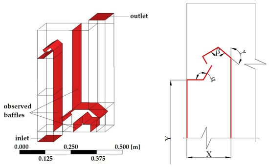
Figure 1.
The model of the proposed flue gas tract: (I) X: width, (II) Y: height, (III) α, β, γ: angles.
The first position of the first baffle used was 80 mm from the wall and an unchangeable height of 400 mm. At the end of the straight part of the baffle was a curvature which directs the flow of flue gases. The model settings were modified by changing the following parameters: (I) width X, (II) height Y, (III) angle α, (IV) angle β, and (V) angle γ. The values of changeable parameters are stated in Table 1.

Table 1.
The changeable parameters of the baffle.
The meshes of the observed models are shown in Figure 2. The shape of mesh elements was mostly hexagonal in all proposed settings. The number of elements, and the average values of the orthogonal quality, the skewness, and the aspect ratio are stated in Table 2. Based on the data stated in Table 2, the mesh quality was evaluated as acceptable to the criteria in all proposed settings.
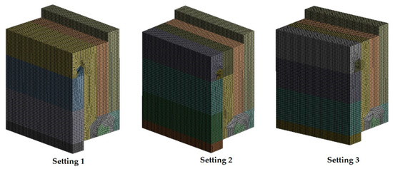
Figure 2.
The meshes of the observed models.
Table 2.
The mesh quality.
Wall boundary conditions were set up for individual parts of baffles. The CFD model was developed in Ansys software (ANSYS, Inc., Canonsburg, PA, USA), where the CFD solver was Ansys Fluent.
Boundary conditions are stated in Table 3. The velocity of the flue gas was set up for the inlet and the pressure was set up for the outlet. Firstly, the mass flow in the inlet was evaluated by stoichiometric calculations with a consideration of 15 kW heat power. The simulation was considered with the fuel of wood pellets. Their characteristics were as follows: (I) 49.8% of carbon, (II) 6.4% of hydrogen, (III) 0.3% of nitrogen, (IV) 10% of moisture, (V) 0.8% of ash, and (VI) 15.4 MJ.kg−1 of calorific value [19]. The inlet velocity was converted from the determined mass flow using the continuity equation. However, after recalculating the velocity into the flue gas tunnel leading to the model, it was not possible to achieve an experimental velocity of 1.97 m∙s−1 resulting from the stoichiometric calculations. Therefore, the measurements were performed at the minimum velocity achievable in the experimental set-up, which was 2.5 m∙s−1. The simulations were performed at this velocity converted to the area in the inlet of the model. They were realized at a temperature of 20 °C, the same as during the experimental measurement, without including the combustion process. The air density was set at 1.18 kg∙m−3 due to a temperature of 20 °C. Outlet pressure was evaluated at −12 Pa according to STN EN 13240.
Table 3.
Boundary conditions.
The simulation of particulate matter motion in the flue gas was performed using a two-phase model. The airflow was simulated using the Navier–Stokes equations. Lagrangian particle tracking was used for particle motion, which is stated in Equation (1).
where Fx is an additional acceleration [m∙s−2], FD is the drag force [s−1], u is the fluid velocity [m∙s−1], ρ is the fluid density [kg∙m−3], up is the particle velocity [m∙s−1], and ρp is the particle density [kg∙m−3] [20].
The particle size distribution was performed using the Rosin–Rammler exponential equation, which is given in Equation (2). The size range was divided into several discrete intervals, this interval representing the mean average for which the trajectories were calculated.
where Yd is a volume fraction of particles with a diameter larger than d, is the mean parameter, and n is the spread parameter [20]. An experimental particle size distribution had to be performed to solve this equation. It was realized using a vibrating sieve shaker with the following results: (I) 10.8% particles with a diameter less than 20 µm, (II) 31.65% particles with a diameter between 20 and 50 µm, (III) 35.61% particles with a diameter between 50 and 100 µm, (IV) 14.83% particles with a diameter between 100 and 150 µm, (V) 6.68% particles with a diameter between 150 and 250 µm, and (VI) 0.43% particles with a diameter between 250 and 500 µm [21].
The simulation was realized by using the k–ε realizable model with a scalable wall function. The combustion process was not included in this model. The model was simulated by considering the temperature of 20 °C, which was reached during the experimental measurement.
2.2. PIV Measurement
The CFD model was verified by PIV measurement. The experimental set-up consisted of the model with baffles created based on the CFD simulations, a closed air tunnel to ensure the flow conditions, and the equipment needed for the PIV method. The model of the flue gas tract was inserted into the fiberboard. This model was constructed from transparent polymethyl methacrylate (PMMA) material, which was connected using metal elements. The dimensions of the model were the same as when using the CFD, and the settings of the model were also modified in the same way.
The closed air tunnel consisted of a flow fan, a differential pressure sensor for setting the fan operating velocity, a temperature sensor for controlling the flow conditions, an anemometer for measuring and setting the airflow velocity, a droplet generator that produced and distributed a tracer in the form of oil droplets to the air tunnel, and a logger. Oil droplets represented the particulate matter. The experimental set-up is shown in Figure 3.
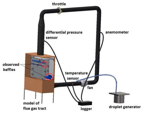
Figure 3.
The experimental set-up.
PIV equipment included a charge-coupled device (CCD) camera, a neodymium-doped yttrium aluminum garnet (Nd: YAG) laser, and the Dynamic Studio software for the evaluation measurements. Oil droplets were illuminated by the Nd: YAG laser. The main laser beam had a wavelength of 1064 nm, and the second laser beam with a wavelength of 532 nm was found in the spectrum of green light. The laser beam was transformed into a divergent laser light sheet by light sheet optics. The CCD camera recorded the figures at each pulse. This camera was rotated 90° from the laser plane and also equipped with a filter that let through only green particles. PIV equipment is shown in Figure 4.
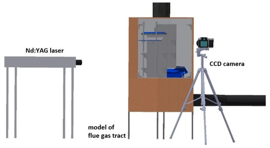
Figure 4.
PIV equipment.
The measurement was realized in a dark room without the influence of other light sources. The first measurement area was located at the top of the model, where the first baffle was curved. These measurements were realized with three different settings of the baffle. The second measurement area was realized in the place of the divide of the second baffle. The measurement realized in this area was only for setting 1. Before the start of the measurements, it was necessary to calibrate the camera and select points A and B. Based on these points, the scale was determined. The velocity of flowing oil droplets in the tunnels reached 2.5 m∙s−1. The camera exposure time was set to 300 µs. Depending on the flow velocity, the time between figures was also set to 450–900 µs. The optimal displacement of the particles in the evaluation area should not be greater than 8 pixels. In this case, the maximum displacement was 6 pixels during the measurement between the two figures. The laser intensity should be adjusted so that the figure quality from the first laser and the second laser is the same. Based on the visibility of the particles and the number of shading and obstacle elements, the intensity of the first laser was set to 5.7–6.2 and the intensity of the second laser 6.0–6.3. Firstly, the size of the evaluated area was 16 × 16 pixels. Then, if no particle was found, the area was gradually enlarged to 64 × 64 pixels. The size of the evaluation area was determined so that all particles were recorded.
The Dynamic Studio software (Dantec Dynamics A/S, Skovlunde, Denmark) used two figures from the measurement, the correlation, a mask, and the removal of erroneous vectors with the use of the range, peak, and moving average. The result is the time middle-average vector velocity field, which is created from all validated instantaneous states of the velocity field in a given set of measurements.
Figure records of PIV measurements were evaluated by mathematical statistics, which were correlations between two consecutive images. The measurement uncertainty is expressed by a correlation coefficient with a range from 0 to 1, where 0 means the match is 0% and it was not possible to identify the particle shift between frames, and 1 represents 100% correlation certainty. The value of the correlation coefficient is influenced, among other things, by the quality of the image recording, poorly lighted measured areas, too large a variance of velocities in the monitored space, and the formation of lost pairs. Lost pairs are caused by the incapability to identify a particle in the interrogation area on two consecutive frames, and this can be caused by the incorrect setting of time between laser pulses, when the particle shift is greater than the maximum allowable value of 8 pixels, large velocity variability in the monitored area, significant 3D flow, etc.
During the experimental measurements, a correlation coefficient was achieved in the range of 0.96 to 0.98 in the main monitored areas, which can be considered as a very accurate measurement. A more significant error was in poorly lighted parts of the monitored areas, where the correlation coefficient achieved a value in the range of 0.82 to 0.87. Poorly lighted areas represented shadows behind the baffles.
3. Results
3.1. CFD Analysis
The velocity was the main observed parameter. Velocity distribution is shown in Figure 5. The size range of velocity is from 0 to 1.5 m∙s−1, the same as in the PIV results. The highest velocity is achieved in setting 1 with the value of 2.3 m∙s−1. At settings 2 and 3, it is decreased to 2.1 m∙s−1. The higher velocities are reached in the narrowest section at the end of the first baffle. Behind the narrowest section, velocities in all settings are close to 1.2 m∙s−1. Velocities reach up to 1.5 m∙s−1 in the places near the wall.
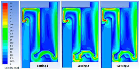
Figure 5.
The velocity distribution based on the CFD.
At setting 1, the velocity reaches a value of 0.6 m∙s−1 in the area of the bend of the second baffle. During the section between the second and third baffles, the velocity increases to 0.9 m∙s−1 and then gradually decreases to 0.7 m∙s−1. The velocity increases again to 0.9 m∙s−1 at the end of the second baffle. At settings 2 and 3, the velocities are slightly higher due to the narrower section between the wall of the first and second baffles.
The impact of the changeable parameters of the baffle is stated in Table 4. Results show that the most effective setting is number 1 due to the most captured particles based on their number. Setting 2 can capture 1.8% less particles and setting 3 can capture 0.6% less particles than setting 1.
Table 4.
The impact of changeable parameters of the baffle.
The amount of captured particles will, in fact, be higher than that stated in Table 4. The results were considered with a higher velocity than indicated by the stoichiometric calculations. A higher velocity was used due to experimental possibilities. In terms of simulation involving stoichiometric calculations, up to 62.3% of particles would be captured in setting 1.
3.2. PIV Analysis
The velocity distribution obtained from the first measurement area is shown in Figure 6. The individual scalar maps have a similar characteristic of the flow. The velocities begin to increase beyond the narrowed section and reach up to the value of 1.1 m∙s−1. The area of the narrowest section was not illuminated very well due to the presence of different shadows. Therefore, velocities in this area could not be accurately measured. It can be summarized that the real velocities in the narrowest section may be significantly higher.
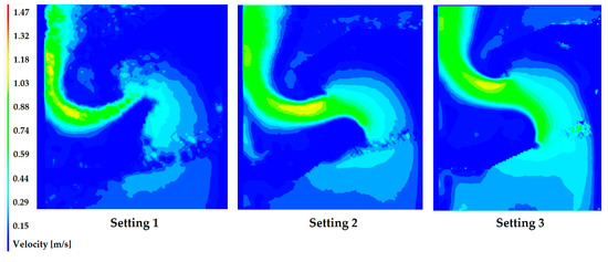
Figure 6.
The velocity distribution based on the PIV from the first measurement area [22].
The velocity distribution obtained from the second measurement area is shown in Figure 7. The size range of velocity is from 0 to 0.69 m∙s−1 due to the better clarity of the figure. At setting 1, the velocities reach a maximum value of 0.55 m∙s−1 but a local increase in velocity can be observed at the end of the second baffle, where the velocity is 0.68 m∙s−1.
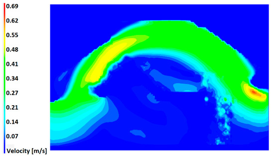
Figure 7.
The velocity distribution based on the PIV from the second measurement area.
In Figure 8, streamlines in all settings can be seen. The strongest stream can be observed in setting 3, which may mean the most escaped particles. However, the greatest vortexes can be seen in this setting. The more vortexes arise, the more areas there are for the settling of particles. Therefore, vortexes present a potential for capturing particulate matter. The smallest vortexes can be seen in setting 1, but also the weakest stream. In setting 2, there are a stronger stream and greater vortexes than in setting 1, but a weaker stream and smaller vortexes than in setting 3.
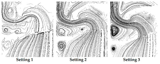
Figure 8.
Streamlines from the first measurement area [22].
In the second measurement, vortexes formed mainly below the third baffle, but also at the point of bending above this baffle, which is shown in Figure 9.
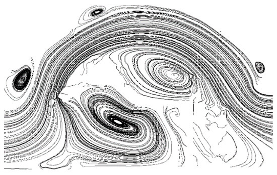
Figure 9.
Streamlines from the second measurement area.
3.3. Comparison of Results from CFD and PIV
For PIV measurements in the first measurement area, the highest velocities of 1.1 m∙s−1 were reached. In the cases of CFD simulations, the highest velocities of 2.1–2.3 m∙s−1 were achieved. However, the area of the narrowest section was not illuminated during PIV measurement very well due to the presence of different shadows. Therefore, velocities in this area could not be accurately measured, and they may be significantly higher. In the area behind the narrowest section, the velocities in CFD simulations were close to 1.2 m∙s−1, and only in the places near the wall did values reach up to 1.5 m∙s−1.
For PIV measurements in the second measurement area, velocities up to 0.55 m∙s−1 were reached, but with a local increase in the velocity with a value of 0.68 m∙s−1 at the end of the second baffle. In the cases of CFD simulations, velocities reached a value of 0.6 m∙s−1 in the area of the bend of the second baffle, then the velocity increased up to 0.9 m∙s−1 and gradually decreased to 0.7 m∙s−1. The velocity increased again to 0.9 m∙s−1 at the end of the second baffle.
For better velocity comparison, velocity graphs were created in the cross-section by a line A-A’ behind the first baffle at the height of 415 mm from the bottom edge of the model, and at a distance of 60 mm from the front wall of the model inwards. The cross-section A-A’ is stated in Figure 10.
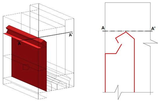
Figure 10.
The cross-section by a line A-A’.
These graphs for setting 1 are shown in Figure 11. The velocity profile obtained by the CFD simulation is smoother due to the idealized flow in the model. The highest velocity in CFD reached in the cross-section is about 1.4 m∙s−1. The velocity profile from the PIV measurement is the velocity of the oil droplets. The flow of these particles is influenced by their mutual interaction and measurement conditions. Their profile is not as smooth as in CFD simulation. The highest velocity in PIV reached in the cross-section is about 1.1 m∙s−1. Despite these differences, the stated graphs have a similar character with increasing velocities up to a distance of about 10 mm from the model wall, and then the velocities gradually decrease. For the other two settings, the graphs are similar to setting 1 and shown in Figure 12 and Figure 13.
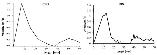
Figure 11.
Velocity graphs in cross-section behind the first baffle for setting 1.
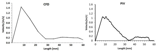
Figure 12.
Velocity graphs in cross-section behind the first baffle for setting 2.
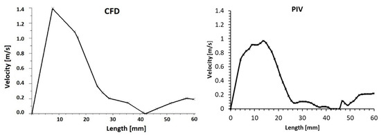
Figure 13.
Velocity graphs in cross-section behind the first baffle for setting 3.
Velocity graphs in the cross-section A-A’ behind the first baffle for setting 2 are shown in Figure 12. The highest velocity in CFD is, in this cross-section, almost 1.5 m∙s−1 and in PIV, almost 1.1 m∙s−1. These graphs have a similar character again with increasing velocities up to a distance of about 10 mm from the wall, and then the velocities gradually decrease.
Velocity graphs in the cross-section A-A’ behind the first baffle for setting 3 are shown in Figure 13. The highest velocity in CFD reaches about 1.4 m∙s−1 and in PIV it reaches about 1.0 m∙s−1. The character of the flow is similar again to that for settings 1 and 2. The velocities increase up to a distance of about 10 mm from the wall and then gradually decrease.
Compared to the PIV results with CFD simulations, velocities measured by the PIV method are lower. These differences could be caused due to lost pairs. Faster particles may lose a pair more often because they have a greater shift in the figure plane. As a result, lower velocities may be measured compared to what they actually are [23]. Other inaccuracies in the results could be caused by shadows formed on the edges or connections of individual parts of the model, or other opaque parts. The resulting differences could also be due to the use of oil droplets during the PIV measurement, while ash particles were used in CFD simulations. Local insufficient particle saturation during PIV measurements could also arise. In CFD simulations, neither external influences nor material properties of the model were considered, which could lead to further deviations. Despite these differences, the characteristic of the flow in CFD and PIV cases is very similar.
4. Conclusions
The reduction in particulate matter during combustion can be achieved by optimizing the flue gas flow. This is important in terms of its impact on human health. This article deals with the optimization of the flue gas flow using three separation baffles located in the flue gas tract. The geometric parameters of the first separation baffle were changed and their influence was investigated using CFD simulations and PIV measurements.
Based on CFD simulations, the results showed that the most effective is setting 1. Setting 2 can capture 1.8% less particles and setting 3 can capture 0.6% less particles than setting 1. In terms of stoichiometric calculations, it would be possible to capture up to 62.3% of the particles. Based on PIV measurements, the results showed the greatest vortexes arising at setting 3, but the weakest flue gas stream at setting 1.
The comparison of PIV measurements and CFD simulations confirmed the supposed character of the turbulent flow with vortexes appearing in the flue gas tract. Inaccuracies in PIV measurements that lead to a decrease in the measured velocity could be due to the lost pairs, shading elements, or local insufficient particle saturation. In CFD simulations, higher velocities were achieved. They were idealized, and the flow of flue gas was unaffected by external influences or material properties. The results, despite the mentioned inaccuracies, are sufficient to follow this problem.
Based on the results, it can be concluded that CFD is a suitable tool for optimizing the flue gas flow during combustion, and PIV can be used for validation of this flow, similar to what has also been mentioned in various other works. To obtain more accurate results, it would be appropriate to include the effect of the combustion temperature, which could be a part of future research.
Author Contributions
N.Č.K., investigation, conceptualization, writing—original draft; A.Č., writing—review and editing, data curation; M.P., data curation; M.H. and P.Ď., formal analysis. All authors have read and agreed to the published version of the manuscript.
Funding
This publication was produced with the support of the Integrated Infrastructure Operational Program for the project: Creation of a Digital Biobank to support the systemic public research infrastructure, ITMS: 313011AFG4, co-financed by the European Regional Development Fund and VEGA 1/0233/19: Construction modification of the burner for combustion of solid fuels in small heat sources.
Institutional Review Board Statement
Not applicable.
Informed Consent Statement
Not applicable.
Data Availability Statement
Data available in a publicly accessible repository.
Conflicts of Interest
The funders had no role in the design of the study; in the collection, analyses, or interpretation of data; in the writing of the manuscript, or in the decision to publish the results.
References
- Sippula, O. The influence of wood fuel chemical composition on particulate emissions. In Proceedings of the Reduction of Fine Particle Emissions from Residential Wood Combustion, Kuopio, Finland, 22–23 May 2006; pp. 10–12. Available online: https://www.osti.gov/etdeweb/biblio/20956140 (accessed on 22 February 2021).
- Nosek, R.; Tun, M.M.; Juchelkova, D. Energy Utilization of Spent Coffee Grounds in the Form of Pellets. Energies 2020, 13, 1235. [Google Scholar] [CrossRef]
- Fullova, D.; Durcanska, D.; Jandacka, D.; Estokova, A. Mass Distribution of Particulate Matter Produced During Abrasion af Asphalt Mixtures in Laboratory. Communications 2016, 18, 37–43. [Google Scholar]
- Karagulian, F.; Belis, C.A.; Dora, C.F.C.; Prüss-Ustün, A.M.; Bonjour, S.; Adair-Rohani, H.; Amann, M. Contributions to cities’ ambient particulate matter (PM): A systematic review of local source contributions at global level. Atmos. Environ. 2015, 120, 475–483. [Google Scholar] [CrossRef]
- European Environment Agency. Air Quality in Europe—2020 Report; No 09/2020; European Environment Agency: Copenhagen, Denmark, 2020; ISSN 1977-8449. [Google Scholar]
- Miricioiu, M.G.; Niculescu, V.C. Fly Ash, from Recycling to Potential Raw Material for Mesoporous Silica Synthesis. Nanomaterials 2020, 10, 474. [Google Scholar] [CrossRef] [PubMed]
- Bianco, V.; Szubel, M.; Matras, B.; Filipowicz, M.; Papis, K.; Podlasek, S. CFD analysis and design optimization of an air manifold for a biomass boiler. Renew. Energy 2021, 168, 2018–2028. [Google Scholar] [CrossRef]
- Smith, J.D.; Sreedharan, V.; Landon, M.; Smith, Z.P. Advanced design optimization of combustion equipment for biomass combustion. Renew. Energy 2020, 145, 1597–1607. [Google Scholar] [CrossRef]
- Nussbaumer, T.; Kiener, M.; Horat, P. Fluid dynamic optimization of grate boilers with scaled model flow experiments, CFD modeling, and measurements in practice. Biomass Bioenergy 2015, 76, 11–23. [Google Scholar] [CrossRef]
- Athanasios, N.; Nikolaos, N.; Nikolaos, M.; Panagiotis, G.; Kakaras, E. Optimization of a log wood boiler through CFD simulation methods. Fuel Process. Technol. 2015, 137, 75–92. [Google Scholar] [CrossRef]
- Silva, J.; Teixeira, J.; Teixeira, S.; Preziati, S.; Cassiano, J. CFD Modeling of Combustion in Biomass Furnace. Energy Procedia 2017, 120, 665–672. [Google Scholar] [CrossRef]
- Gómez, M.A.; Martín, R.; Chapela, S.; Porteiro, J. Steady CFD combustion modeling for biomass boilers: An application to the study of the exhaust gas recirculation performance. Energy Convers. Manag. 2019, 179, 91–103. [Google Scholar] [CrossRef]
- Zadravec, T.; Rajh, B.; Kokalj, F.; Samec, N. CFD modelling of air staged combustion in a wood pellet boiler using the coupled modelling approach. Therm∙Sci. Eng. Prog. 2020, 20, 100715. [Google Scholar] [CrossRef]
- Bastiaans, R.J. Cross-Correlation PIV: Theory, Implementation and Accuracy; Faculty of Mechanical Engineering, Eindhoven University of Technology: Eindhoven, The Netherlands, 2000; ISBN 90-386-2851-X. [Google Scholar]
- Mizeraczyk, J.; Kocik, M.; Dekowski, J.; Dors, M.; Podlinski, J.; Ohkubo, T.; Kanazawa, S.; Kawasaki, T. Measurements of the velocity field of the flue gas flow in an electrostatic precipitator model using PIV method. J. Electrost. 2001, 51–52, 272–277. [Google Scholar] [CrossRef]
- Sung, Y.; Choi, G. Non-intrusive optical diagnostics of co- and counter-swirling flames in a dual swirl pulverized coal combustion burner. Fuel 2016, 174, 76–88. [Google Scholar] [CrossRef]
- Schneider, H.; Valentiner, S.; Vorobiev, N.; Bohm, B.; Schiemann, M.; Scherer, V.; Kneer, R.; Dreizler, A. Investigation on flow dynamics and temperatures of solid fuel particles in a gas-assisted oxy-fuel combustion chamber. Fuel 2021, 286, 119424. [Google Scholar] [CrossRef]
- Nussbaumer, T.; Kiener, M. Moving grate combustion optimization with CFD and PIV. In Proceedings of the 21st European Biomass Conference and Exhibition, Copenhagen, Denmark, 3–7 June 2013. [Google Scholar]
- Desideri, U.; Fantozzi, F. Technologies for Converting Biomass to Useful Energy; CRC Press: Boca Raton, FL, USA, 2017; 520p. [Google Scholar]
- Ansys Fluent Theory Guide. Available online: www.pmt.usp.br (accessed on 22 February 2021).
- Čajová Kantová, N.; Sladek, S.; Jandačka, J.; Čaja, A.; Nosek, R. Simulation of Biomass Combustion with Modified Flue Gas Tract. Appl. Sci. 2021, 11, 1278. [Google Scholar] [CrossRef]
- Čaja, A.; Patsch, M.; Backa, A. PIV Observation of the Baffle Position in the Flue Gas Tract for Particle Flowing. MATEC Web Conf. 2020, 328, 5. [Google Scholar] [CrossRef]
- Kopecký, V. Laserová Anemometrie v Mechanice Tekutin; Tribun EU: Brno, Czech Republic, 2008; ISBN 978-80-7399-357-3. [Google Scholar]


Publisher’s Note: MDPI stays neutral with regard to jurisdictional claims in published maps and institutional affiliations. |
© 2021 by the authors. Licensee MDPI, Basel, Switzerland. This article is an open access article distributed under the terms and conditions of the Creative Commons Attribution (CC BY) license (http://creativecommons.org/licenses/by/4.0/).