Abstract
In the preliminary stages of design of the oscillating water column (OWC) type of wave energy converters (WECs), we need a reliable cost- and time-effective method to predict the hydrodynamic efficiency as a function of the design parameters. One of the cheapest approaches is to create a multiple linear regression (MLR) model using an existing data set. The problem with this approach is that the reliability of the MLR predictions depend on the validity of the regression assumptions, which are either rarely tested or tested using sub-optimal procedures. We offer a series of novel methods for assumption diagnostics that we apply in our case study for MLR prediction of the hydrodynamics efficiency of OWC WECs. Namely, we propose: a novel procedure for reliable identification of the zero singular values of a matrix; a modified algorithm for stepwise regression; a modified algorithm to detect heteroskedasticity and identify statistically significant but practically insignificant heteroscedasticity in the original model; a novel test of the validity of the nullity assumption; a modified Jarque–Bera Monte Carlo error normality test. In our case study, the deviations from the assumptions of the classical normal linear regression model were fully diagnosed and dealt with. The newly proposed algorithms based on improved singular value decomposition (SVD) of the design matrix and on predicted residuals were successfully tested with a new family of goodness-of-fit measures. We empirically investigated the correct placement of an elaborate outlier detection procedure in the overall diagnostic sequence. As a result, we constructed a reliable MLR model to predict the hydrodynamic efficiency in the preliminary stages of design. MLR is a useful tool at the preliminary stages of design and can produce highly reliable and time-effective predictions of the OWC WEC performance provided that the constructing and diagnostic procedures are modified to reflect the latest advances in statistics. The main advantage of MLR models compared to other modern black box models is that their assumptions are known and can be tested in practice, which increases the reliability of the model predictions.
1. Introduction
One of the significant renewable energy sources is wave energy [1]. Wave energy converter (WEC) devices are excited by incident water waves, which create forces between an absorber and a reaction point. Those forces either directly empower a generator or drive a working fluid through a pump. For a feasibility or proof-of-concept study of a WEC device we need accurate predictions of its hydrodynamic efficiency under different design parameters. However, the full commercialization of large-scale WEC is not reached with the oscillating water column (OWC) devices considered the most promising in that regard [2]. The reason is that the latter “is arguably one of the most simple and elegant in design and principle in operation” (as mentioned in [3]) which can reduce its maintenance cost. That is why new investigations are needed in the hydrodynamic efficiency prediction of OWC devices.
Physical model testing is arguably the most accurate approach for estimating wave-induced loads and response of fixed and floating objects including OWC devices [4,5,6,7]. Using physical experiments, measured datasets are collected which connect some design parameters and experimental conditions with the performance measures of the tested OWC devices. The validity of such an approach is based on limited explicitly formulated assumptions, which ensure high confidence in the acquired measured datasets. The experimental data are often used for training and/or validation of numerical models recently developed to predict the performance of WECs. However, the experimental approach has several limitations such as near-fields effects (boundary conditions) and scaling effects. Hence, the measured values will unavoidably contain some random and systematic uncertainties. The results are often sensitive to minor changes in the test conditions and will vary even when several identical replicas are measured. Furthermore, model testing is overly expensive and takes an unreasonably long time to complete. In practice, it is used as a last resort for very expensive devices which have lasting economic or environmental effect. According to the Specialist Committee on Testing of marine Renewable Devices, it is recommended to use large-scale models of power take-off systems to overcome the limitations [8]. Some limitations of the existing model testing facilities were reported in the experimental study in [9].
The numerical models can be divided into three categories (white boxes, grey boxes, and black boxes) according to the knowledge about the modelled physical process utilized in the prediction of the output values (the response) from the values of the input variables (the stimulus).
The white box methods used in the WEC design almost entirely apply the computational fluid dynamics (CFD) approach. Those numerical analysis methods solve a version of the Navier–Stokes to compute the wave-induced loads, hydrodynamic characteristics, and response of WEC devices subjected to unidirectional regular waves [1,10,11,12,13]. The CFD methods use comprehensive numerical schemes to solve the entire system of mathematical equations and demonstrate three advantages in comparison with the physical modelling: they are more time and cost effective, and they have no scaling limitations. Nonetheless, the validation of the CFD-based codes require experimental datasets [3,6,14]. However, the main disadvantage of the CFD technique is that it still takes too much time and expertise to obtain satisfactory results, in particular, with irregular wave cases. The use of CFD-based methods for practical WEC applications is limited to the final stages of design. To address those shortcomings, various simplified numerical models have been proposed based on potential flow models [15]. However, although they perform faster than CFD-based codes, they may produce inaccurate predictions since they ignore viscosity effects, air entrapment phenomenon, and the influence of higher order waves. For instance, using potential-flow-based techniques [16], the hydrodynamic efficiency of an OWC device is often over-predicted [17]. Nowadays, the use of CFD methods for practical WEC applications is limited to the final stages of design, if at all.
The grey box methods are not very popular for the OWC design. The only emerging exception is a method based on the adaptive neuro-fuzzy inference system (ANFIS) which have been applied to different types of WEC devices [18,19]. It combines a multilayer artificial neural network (ANN) with fuzzy logic. The latter allows us to apply “if-then” rules with linguistic terms rather than rules with crisp numerical values [20]. Fuzzy logic is useful in problems containing inaccuracy, where the propositions have a degree of membership (between 0 and 1) to the set of the true propositions as in [21,22]. ANFIS uses fuzzy and partial knowledge (coded in the fuzzy “if-then” rules) about the modelled physical process. The outcome of ANFIS can be partially explained and is easier to interpret than the prediction methods. On the negative side, ANFIS does require dataset for training the model construction. The greatest shortcoming of the approach is that its effectiveness is based on comprehensive expert knowledge about WEC systems. Such sets of “if-then” rules are problem specific and are expensive and time-consuming to acquire.
The black box (BB) methods only aim to approximate the measured output for different inputs based on an information in a known dataset. No knowledge about the modelled physical process is used. There are numerous types of BB methods, but only two types are relevant for the WEC design: ANN and multiple linear regression (MLR).
ANN is a supervised predictive method capable universally completely to approximate any multi-dimensional output function of continuous and discrete input variables, as proven in a theorem [23]. It has proved to be efficient in modelling complex engineering relationships encoded in datasets [24] and were applied to numerous coastal engineering problems [25], including to WEC applications [10]. The advantages of ANN in comparison with the other methods are that they are cheap, fast to predict and easy to realize due to their independence from the modelled process [26]. On the negative side, the complexity of the modelling function often prevents extraction of relevant information suitable to identify the analytical function derived by the ANN. The complex structure of ANN is determined by the so-called hyper-parameters (e.g., the number of hidden layers, the number of neurons in each hidden layer, etc.), which are determined using a validation set. Therefore, the available data set in ANN has to be partitioned into three parts: training, validation and testing part. This additionally complicates the construction of a reliable ANN model when the available data set is not large. Overfitting may result in an ANN model trained over the uncertainties of the observations instead on their useful signal. It is typical of problems with small to medium dataset [10]. A wide variety of regularization techniques [27] and cross validation procedures [28] are developed to reduce the overfitting in ANN, some of them achieving great results. The training of an ANN is a random hyper-dimensional optimization process which takes a long time to train. As a by-product the predicted residuals described in Section 3.1 are rarely calculated in practical problems. However, the main shortcoming of an ANN prediction is the unreliable prediction for any input absent in the training or testing sets. Evidently, ANN is a great tool that constantly evolves, yet its use requires a very high level of expertise, which is often absent with engineering designers.
The MLR method is by far the best-known BB model, with numerous applications to develop predictive models in various engineering tasks (see [29,30,31]). It uses approximation function of multiple variables which is linear according to the unknown parameters. Given a known dataset, the construction of an MLR predictor is very cheap and extremely fast in comparison with the other methods. It also provides a measure of the uncertainty in its prediction. On the negative side, although in most cases the precision of MLR models is enough for engineering purposes, it is as a rule lower than that of the ANN models [32]. However, the main shortcoming of MLR models is that their quality depends on the validity of several restrictive assumptions, which rarely hold in their entirety in any practical application. The actual popularity of MLR in engineering practice is not properly reflected in recent published works, where such models are utilized most often as a basic benchmark. As a result, more and more engineering practitioners tend to use methods they are not fully familiar with and with assumptions that are often violated. The MLR is a useful tool in a variety of problems, yet it should not be used in its basic form that may generate unreliable results as the assumptions are violated (see Section 3.2 for more discussion).
In this paper, we shall develop a reliable and cost-effective MLR prediction of the hydrodynamic efficiency of the OWC as a function of the construction parameters using an existing data set. Such a model would be useful in the preliminary stages of design of WECs, but its reliability strongly depends on the validity of the classical linear regression assumption. We will introduce a series of novel/modified methods for assumption diagnostics that share two features: the repeated application of an improved singular value decomposition (SVD) of the design matrix using novel classification of the singular values, and the universal use of the predicted residuals. We shall propose: a novel procedure for reliable identification of the zero singular values of a matrix; a modified algorithm for stepwise regression; a modified algorithm to detect heteroskedasticity and identify statistically significant but practically insignificant heteroscedasticity in the original model; a novel test of the validity of the nullity assumption; a modified Jarque–Bera Monte Carlo error normality test; and a novel multiple testing outlier procedure with two phases in each cycle. We will investigate the correct placement of the outlier detection in the overall diagnostic sequence empirically. A new family of goodness-of-fit measures and the aforementioned outlier detection procedure are also based on predicted residuals. We will use predicted residual based modified performance indicators to demonstrate that the developed MLR model can produce highly reliable predictions of the OWC WEC hydrodynamic efficiency, provided that the construction and diagnostic procedures are modified to reflect the latest advances in statistics. The case study that we shall analyze will demonstrate how these algorithms behave in an actual engineering data set, as opposed to demonstrating them in generated data sets.
In what follows, Section 2 will describe the origin and the experimental settings of the measured dataset. In Section 3.1 we will introduce the rationale of the new performance measures for general BB models. In Section 3.2 we will recall how the classical assumptions facilitate the construction of the standard MLR model. Section 3.3 will introduce the modified procedure for testing and relaxing each of the classical assumptions. The outlier testing procedure and its place in the overall diagnostic procedure is discussed in Section 3.4. In Section 4, we construct four MLR models predicting the OWC hydrodynamic efficiency and compare their performance measures. Section 5 concludes the paper.
2. Oscillating Water Column (OWC) Wave Energy Converter (WEC) Benchmark Test
The efficiency of the OWC WEC depends greatly on the amount of air trapped in the device, and the amount of wave energy that causes the movement of the WEC. To develop our prediction models, we will use the experimental dataset in [33] where the hydrodynamic efficiency of fixed OWC wave energy devices are measured under various wave conditions and variable geometric characteristics of the devices. In Figure 1, a sketch of the experimental setting is shown which was designed to investigate the effect on the hydrodynamic efficiency of five variables. The variable x1 is the unitless wavenumber of the incident waves with constant amplitude of 0.03 m, which were generated by the wave-maker. The still water depth h was 0.8 m during the experiment and therefore x1 = K = (2πh)/λ = (1.6π)/λ for a wave with wavelength λ [m]. The variables x2 = B, x3 = d, x4 = D, and x5 = θ describe the geometry of the OWC WEC device (see Figure 1). The names, the measurement units, and experimental values of the independent variables are given in Table 1. For simplicity, the input variables can be organized in 5-dimensional column vector of independent input where T stands for transpose. The dependent variable y being the efficiency of the OWC WEC device was calculated as the ratio of the hydrodynamic energy absorbed by the waves for time τ and the energy contained in the incident waves for time τ, where τ is one wave period. We will use a data set consisting of 126 records where the ith record contains the measurement, yi, of dependent variable (the efficiency) under experimental conditions determined by the values of the independent variables xi1, xi2, xi3, xi4, and xi5. Since the latter form a vector of independent input , the ith record in the dataset is the couple . Refer to [33] for more details about the experimental setting of the wave flume and about the dataset formation.
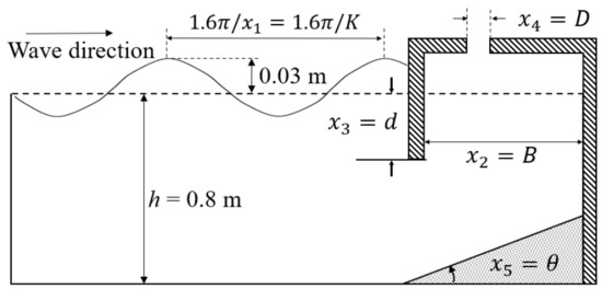
Figure 1.
Definition sketch for the independent variables (simplified from [15]: reprinted from Energy Vol 83, De-Zhi Ning, Jin Shi, Qing-Ping Zou, Bin Teng, Investigation of hydrodynamic performance of an OWC (oscillating water column) wave energy device using a fully nonlinear HOBEM (higher-order boundary element method), Pages 177-188, Copyright 2015, with permission from Elsevier.).

Table 1.
Description of the independent variables.
The 126 records in the data set are divided into 9 groups of 14 records each. The experimental group k (for k = 1, 2, …, 9) contains the records i = 14k−13, 14k−12, …,14k. In each group the 14 records have the consecutive unitless values of xi,1 = K as shown in the last column of Table 2. The values of xi,2 = B are 0.7 m for group 2, 0.85 m for group 3, and 0.55m otherwise. The values of xi,3 = d are 0.17 m for group no. 4, 0.20 m for group no. 5, and 0.14 m otherwise. The values of xi,4 = D are 0.04 m for group no. 6, 0.08 m for group no. 7, and 0.06 m otherwise. The values of xi,5 = θ are 10o for group no. 8, 20 o for group no. 9, and 0 o otherwise. The measured values of the hydrodynamic efficiency, yi, (acquired as in [34]) are shown in the first nine columns of Table 2.

Table 2.
Values of the measured hydrodynamic efficiencies, yi, and of unitless wavenumbers xi,1 = K, where the number of the group is k = 1,2, …, 9.
The discussed data set has unequal distribution of data points in the five-dimensional space of independent variables. In an ideal case, this space should be evenly covered with experiments. Since designers can rarely perform experiments in the early stage of the design, they have to rely on available data sets (previously conducted in different settings). This is a typical challenge when using MLR over existing imperfect data (or any other method).
3. Methodology
3.1. Performance Indicators for Black Box Models
Given the dataset described in Section 2, we can develop different BB models for OWC WEC, which will accept as input the values of the five independent variables from Table 1, organized in a vector of independent input , and as an output will predict the value of the dependent variable (the predicted hydrodynamic efficiency of the OWC WEC) as shown in Figure 2.

Figure 2.
The input-output diagram for a black box (BB) model for hydrodynamic efficiency predictions.
Each model can be created using a training set {, for i = 1, 2, …, n} consisting of n records from the dataset, where n is selected suitable for the particular model. If the model predicts for the input of , then the quantities are called residuals. During the training of the model, three measures of the residual magnitudes are used traditionally: the root mean square error (RMSE), the mean absolute error (MAE) and the coefficient of determination (R2):
In (3), R2 is the ratio of the explained by the model y-variance and initial variance of the dependent variable. It can take any value between negative infinity and 1. Negative R2 shows that the model produces residuals which are generally greater that the “constant response model” which predicts the mean value for any input . The performance indicators (1), (2), and (3) are measures of the resubstitution error of the BB model because the same training set is used to estimate the performance of the model [35]. That is why the former are optimistic in a sense that they indicate better model performance than the actual one. To remedy this situation, we can use a test set {, for i = 1, 2, …,nHO} consisting of nHO records from the dataset which (as a rule) do not belong to the training set for the particular BB model. If the latter predicts for the input of , then the quantities are called predicted residuals [36] (pp. 411–412). If the performance indicators (1), (2), and (3) are estimated for the test set we will get RMSEHO, MAEHO, and . Those three indicators measure the holdout (HO) error of the BB model because the test set to measure the performance of the model has never been used in its training [35]. Hence, RMSEHO, MAEHO, and are unbiased estimates of the actual BB model performance, but their variance increases with the decrease of nHO. As a result, the partition of the dataset into two sets containing n and nHO observations is a question of compromise—we want nHO to be small (to increase maximally its complement n for better training of the model), but simultaneously we want nHO to be large (to decrease the variance of the performance indicators). Usually, this problem is solved by selecting widespread n:nHO partitions such as 70:30, or 80:20. Unfortunately, there is no theoretical justification of those partitions, even though they are widely adopted by engineering practitioners.
3.2. Classical Normal Linear Regression Model
Let Xj be p different functions (called regressors) of the five independent variables:
Xj = gj(x1, x2, x3, x4, x5), for j = 1, 2, …, p
Almost always the regressor X1 is the unity function g1(x1, x2, x3, x4, x5) = 1. Then, we can form a general stochastic regression connection between the efficiency of the OWC and the values of the regressors:
In (5) the dependent variable Y (the hydrodynamic efficiency) is a random variable (r.v.), unlike the regressors Xj (j = 1, 2, …, p) that are non-random observable variables. The error variable, ε, is also considered to be an r.v. and is theoretically responsible for the randomness of Y (although in practice there are other components to this randomness, as discussed after (17) below). The partial regression coefficients β1, β2, …, βp are non-random and unobservable quantities often called slopes. They can be organized in a p-dimensional column vector known as the parameter vector:
When the regressor X1 is the unity function, then β1 is also known as the regression constant. Equation (5) shows how the probability distribution of the r.v. in the left-hand side can be estimated using the right-hand side.
The primary task in a MLR is to find a point estimate for the unobservable parameter vector . That can be solved with the ordinary least square (OLS) method if the following assumptions hold [37] (p. 791):
1. Nullity assumption: the expected value of the error variable is zero, i.e., .
2. Homoskedasticity assumption: the variance of the error variable is constant for any independent variables’ vector , i.e., .
3. Normality assumption: the probability distribution of the error variable is normal, i.e., .
4. Correlation assumption: the errors of the dependent variables are not linearly correlated for any two different independent variables’ vectors, i.e., .
5. Multicollinearity assumption: not a single regressor can be expressed as a linear combination of the rest. If we denote p arbitrary sets, each containing p real numbers with , then the multicollinearity assumption boils down to: .
6. Linearity assumption: the conditional expected value of the dependent variable given some independent variables’ vector is a linear combination of the regressors with coefficients equal to the components of the parameter vector, i.e., .
The sixth assumption, formulated in [38], is often omitted in the set of classical OLS assumptions, but it is an important one. If we use OLS to construct a model like (4) that complies with the six classical assumptions, we will obtain a classical normal linear regression model (CNLRM) [39] (pp. 107–117).
Using the linearity assumption, we can predict a point estimate of the dependent variable as the conditional expected value for any vector of independent input where the predictors are given in (4):
The part (7) from (5) is aka systematic component, whereas the error variable, ε, in (5) is aka stochastic component [40]. Let as calculate the p regressors for the ith records in the dataset using (4):
Then, the information in the experimental dataset can be compactly described by the n-dimensional column vector of the observed values given in (9) and the [n × p]-dimensional design matrix X shown in (10):
In the MLR model, initially the training data set is the whole dataset which means that n = 126. To find an estimate of the unknown parameter vector we can write the MLR model (5) for all records in the data set:
In (11), the n-dimensional column vector of residuals is a function of the unknown parameter vector . Since we want the residuals to be as small as possible, we can find the point estimate of the parameter vector as:
The identification of the coefficient estimates (12) is the essence of the OLS method. The optimization problem (12) has a closed solution [40]:
In (13), the matrix (XTX) is a square [p × p] symmetric matrix (we will call it the information matrix for simplicity). As p << n, the information matrix is expected to have an inverse. According to the Gauss–Markov theorem, (13) is the best linear unbiased estimator (BLUE) for the parameter vector [41] (pp. 358–360). Plugging the point estimate of the parameter vector into (7) we can obtain the MLR model for hydrodynamic efficiency of the OWC WEC as required in Figure 2:
The resubstitution OLS residuals are calculated utilizing (9), (10), (11) and (14):
The n components, ei, of the vector of residuals (15) form a sample containing n known variates of the error variable ε in (5). The sample mean of the resubstitution OLS residuals (14) will always be zero:
Utilizing (16), the sample standard deviation of the resubstitution OLS residuals (14) (aka standard error estimate) can be obtained by:
According to (13), the point estimate of the parameter vector depends on the vector of the observed values . The latter contains n random variates of the dependent variable Y (the hydrodynamic efficiency) which is an r.v. It follows that each component, bi, of is an r.v. and the latter is a random vector. In that sense, the predicted value of the r.v. Y according to (14) is an estimate of the systematic component. Its randomness is determined by the random estimate of the parameter vector , so the randomness of Y is determined both by the randomness of the stochastic component and by the randomness of the estimate of the systematic component. According to [42], the covariance matrix of is a [p × p] symmetric matrix:
From (18), we can find the estimated standard error of the parameter estimates bi as square root of the corresponding diagonal element of :
Using the OLS residuals (15) the model performance resubstitution indicators RMSE, MAE, and R2 can be estimated by (1), (2), and (3). Typically, for the MLR model an adjusted coefficient of determination is used which improves the R2 by considering the degrees of freedom (that is the count of the parameters used in the model):
The resubstitution measure is useful when it is positive, otherwise the developed MLR model is inadequate.
One of the amazing properties of the MLR is that it can cheaply calculate the holdout predicted residual for the ith observation if the MLR model is built using all other observations in the dataset. Such a residual is also known as a leave-one-out (LOO) residual and can be denoted as ei,HO according to Section 3.1:
Here, the ith row of the design matrix (10) is denoted as , which is a p-dimensional row vector [43]. The LOO formula (21) is used n times (once for each record in the dataset), which corresponds to a test set with nHO = n = 126. Then the holdout residuals can be substituted in (1), (2), and (3) to produce the three holdout measures of the MLR data set RMSEHO, MAEHO, and . Each of the predicted residuals ei,HO is obtained by a model MODi, which is marginally worse than the MLR model (14) since MODi neglects the observation in its training set. A particular MODi will be practically the same as the MLR model (14), except in the case when is an outlier and therefore should be neglected altogether. That is why, RMSEHO, MAEHO, and are ever so slightly pessimistically biased estimates of the real model performance (in fact, they are unbiased) but with minimal variance because nHO = n is maximal.
The estimated performance indicators RMSE, MAE, R2, , RMSEHO, MAEHO, and are implicit quantitative measures for the validity of the MLR model. Additionally, an explicit qualitative measure for the validity of our regression model should answer whether its performance is statistically significantly better than the performance of the “constant response model” which predicts the mean value of the hydrodynamic efficiency for any vector of independent input . Let us test the null hypothesis H0 (that all slopes in front of the non-constant regressors are zeros) against the alternative hypothesis H1 (that at least one slope in front of a non-constant regressor is not zero):
The F-test solves the formulated problem by using the test statistics Fstats, which originates from the analysis of variance (ANOVA) approach:
If CDFF,a,b(.) is the cumulative distribution function of the Fisher–Snedecor distribution (aka the F-distribution) with the degree of freedom a as a numerator and with the degree of freedom b as denominator, then the p-value of the test (22) is [36] (pp. 117–118):
3.3. Testing and Relaxing the Classical Assumptions
The validity of the six classical assumption formulated in Section 3.2 will be tested for the constructed MLR model. If an assumption is rejected, whenever possible we will propose corrections in the MLR model that can handle a relaxed assumption. The presentation will follow the algorithmic order in which the assumptions were tested and relaxed during the construction of our MLR model.
3.3.1. Diagnostics of the Multicollinearity Assumption
The multicollinearity assumption is the first one to be tested and relaxed. It requires that the design matrix has a full rank, i.e., rank(X) = p. If that is not the case, then the information matrix, (XTX), will have no inverse and the point estimate of the parameter vector could not be obtained with (13). The solution of this problem can be found in [44] (pp. 788–798) with a proposed 3-step SVD procedure.
Step 1: Factor the design matrix X to the product of three matrices using SVD decomposition:
In (25), U is a [n × p]-dimensional column-orthonormal matrix with columns (for j = 1, 2, …, p), S is a [p × p]-dimensional diagonal matrix with non-negative elements sj (for j = 1, 2, …, p) on the main diagonal, called singular values, and V is a [p × p]-dimensional orthonormal matrix with columns (for j = 1, 2, …, p).
Step 2: Classify the singular values sj (for j = 1, 2, …, p) into ‘positive group’ and ‘zero group’. Set , if sj belongs to the ‘positive group’. Set , if sj belongs to the ‘zero group’.
Step 3: Approximate the inverse of the information matrix as:
The classification in the second step is not trivial. The SVD decomposition (25) is executed by software and therefore subject to round-off errors. We need to judge subjectively which singular values are in fact small positive real values and which are in fact zeros (but estimated as small positive real values due to round-off errors). According to [45], an improved automatic version of the above algorithm can be obtained by substituting its second step with the following procedure for classification and correction of singular values (PCCSV).
| Algorithm 1: Classification and correction of singular values of a matrix (PCCSV) |
| 1. Set j = 1. |
| 2. If , then set and go to step 8. |
| 3. Calculate as an estimate of the unit vector . |
| 4. Estimate the length of as . |
| 5. Estimate the angle in degrees between and as . |
| 6. If and , then set and go to step 8. |
| 7. Set . |
| 8. Set j = j + 1. |
| 9. if , then go to step 2. |
The main idea of PCCSV is that if the jth singular value is really 0, then the vector will be an estimate of the p-dimensional column zero vector, . Then, the vector will be an estimate of which will make it quite different from the unit vector . By contrast, if the jth singular value is really a small positive, then the vector will be an estimate of the unit vector and the two of them will be close both in direction and in magnitude.
If the approximation (26) is used in Formulas (13), (18) and (21), the numerical problems resulting from violation of the perfect multicollinearity assumption will disappear. It can be proven that using (13), (25), and (26) we can obtain a better point estimate of the parameter vector:
The estimate (27) is computationally more expensive than (13) because of the SVD decomposition. However, the robustness of (27) is superior to (13) as it will work reliably even if the design matrix, X, is ill-conditioned or singular.
3.3.2. Diagnostics of the Linearity Assumption
The linearity assumption deals with the selection of regressors and relates to two problems.
The first problem is to identify whether all the regressors in our model contribute to the prediction precision instead of only increasing the noise in the regression. If the linearity assumption holds, for an arbitrary regressor in (5) there should be a meaningful linear relation between the dependent variable and the regressor. Let us test for each j = 1, 2, …, p the null hypothesis (that the regressor Xj does not contribute to the prediction precision) against the alternative hypothesis (that the regressor Xj does contribute to the prediction precision):
The t-test solves the formulated hypothesis test by using the test statistics tstats,j (29), where the standard error of the parameter estimates bj is given in (19):
If CDFt,a(.) is the cumulative distribution function of the Student distribution (aka the t-distribution) with a degrees of freedom, then the p-value of the test (27) is [37] (p. 801):
The test (28) is repeated for each of the regressors in (5), i.e., for j = 1, 2, …, p. In the ideal case all parameters in the regression model will be significant. However, if some of the coefficients are significant but others are not, we cannot simply keep only the regressors with significant coefficients according to the p individual t-tests. The reason is that the model parameters are interconnected and dropping one of them will change both the values and the significance of the other parameters in the new model.
The second problem, related to the linear assumption, is to determine the right structure of the model. We would like to have a model where the linearity assumption holds for each of the regressors and we cannot add any available regressor to the model for which the linearity assumption holds. The stepwise regression is an automatic procedure to select the “correct set” of regressors. It starts with a set of regressor and adds or drops one regressor at each step based on some selection criterion. There are numerous forms of stepwise regression, but the method as such is subjected to criticism, and is summarized as follows:
(a) There is a problem with the significance of individual tests when multiple tests are performed on the same data. For example, of 1000 tests with 5% significance the effect will be false discovered in 50 of them even when the effect is missing.
(b) The selection criterion is very often which makes the stepwise regression to identify smaller regressors sets than the “correct set” of regressors.
(c) Due to the partial multicollinearity the regressors are interconnected and the decision in one step may compromise the choices in the previous steps [39] (p. 378).
(d) If the regression constant b1 (in front of the unit regressor) is treated similarly to the other parameters, it either can be dropped at an earlier step and the dropping decisions in the subsequent steps can be compromised, or it can be added at a later step and the adding decisions in the previous steps can be compromised. If the regression constant b1 is treated differently to the other parameters, we will always end up with model containing the unit regressor even when the regression constant is insignificant which can produce imprecise values of the slopes.
For our model structure we apply a modified stepwise regression algorithm (MSRA) for the MLR, which in our opinion addresses the above issues. That algorithm that follows is based on backward elimination using t-tests as a selection criterion.
| Algorithm 2: Modified stepwise regression algorithm (MSRA) for the MLR |
| 1. Form a list L of regressors containing the unit regressor (g1 = 1), the five linear regressors (g2 = x1 = K, g3 = x2 = B, g4 = x3 = d, g5 = x4 = D, g6 = x5 = θ), the five squired regressors (g7 = x1.x1, g8 = x2.x2, g9 = x3.x3, g10 = x4.x4, g11 = x5.x5), and the ten mixed quadratic regressors (g12 = x1.x2, g13 = x1.x3, g14 = x1.x4, g15 = x1.x5, g16 = x2.x3, g17 = x2.x4, g18 = x2.x5, g19 = x3.x4, g20 = x3.x5, g21 = x4.x5) |
| 2. Set p = 21 and calculate the 21 regressors for each record in the dataset using (8) for i = 1, 2, …, 126 and j = 1, 2,…, 21 |
| 3. Form the initial [126 × 21]-dimensional design matrix X using (10) and the 126-dimensional vector of the observed values using (9) |
| 4. Select the significance level α = 0.05 of the t-tests |
| 5. Perform the SVD decomposition (25) of X and identify: |
| (5a) the 126-dimensional vectors (for j = 1, 2, …, p) |
| (5b) the p-dimensional vectors (for j = 1, 2, …, p) |
| (5c) the singular values sj (for j = 1, 2, …, p) |
| 6. Apply PCCSV and obtain the corrected singular values (for j = 1, 2, …, p) |
| 7. Find the OLS point estimate of the parameter vector using (27) |
| 8. Find the resubstitution OLS residuals using (15) and the standard error estimate using (17), where n = 126 |
| 9. Calculate the [p × p]-dimensional covariance matrix of the model parameters by plugging (26) in (18): |
| 10. Using (19), find the standard errors, se(bj), of the slope estimate bj (for j = 1, 2, …, p) |
| 11. Using (29), find the test statistics, tstats,j, of the jth test (28) for the slope βj (for j = 1, 2, …, p) |
| 12. Using (30), find the p-value, p-valuej, of the jth test (28) for the slope βj (for j = 1, 2, …, p) |
| 13. If the first column of the design matrix X does not correspond to the unit regressor, g1(x1, x2, x3, x4, x5) = 1, then go to step 20 |
| 14. Find j-drop such that p-valuej-drop ≥ p-valuej for j = 2, 3, …, p |
| 15. If p-valuej-drop ≤ α, then go to step 18 |
| 16. Remove the j-drop regressor from the list L, remove the j-drop column of the design matrix X, and set p = p − 1 |
| 17. If p > 1 go to step 5, otherwise go to step 24 |
| 18. If p-value1 ≤ α, then go to step 24 |
| 19. Remove the first regressor from the list L, remove the first column of the design matrix X, set p = p − 1, and go to step 5 |
| 20. Find j-drop such that p-valuej-drop ≥ p-valuej for j = 1, 2, …, p |
| 21. If p-valuej-drop ≤ α, then go to step 24 |
| 22. Remove the j-drop regressor from the list L, remove the j-drop column of the design matrix X, and set p = p − 1 |
| 23. If p > 1 go to step 5 |
| 24. Declare the optimal set or regressors to be in the list L and the optimal design matrix to be the current matrix X. |
In the first step of MSRA, we selected a quadratic model as a second order Maclaurin series expansion of a scalar function (y) of five real variables [46]. This is a typical choice, because it provides enough flexibility to approximate a wide variety of relationships. However, this selection is arbitrary. Researchers can choose such set of regressors that suits their specific case. For example, the square roots of the independent variables can also be added. MSRA can work with any set of regressors that has x1 = 1, as long as the count of the regressors does not exceed roughly half of the count of data points.
The first four instructions of MSRA are initialization of the algorithm, whereas the main body of the procedure consists of instructions 5 to 13. In the main body, we calculate the p-values of the t-tests for significance for all current regressors. It will be executed on every step of the backward elimination procedure. Those steps are divided into three phases. In the first phase (the main body and instructions 14–17), we drop one insignificant regressor per step (selecting the one with maximal p-value), but always keep the regression constant b1 in front of the unit regressor. In the second phase (instructions 18–19), we deal with the unit regressor. If the regression constant b1 is significant, then MSRA stops otherwise we drop the unit regressor. In the third phase (the main body and instructions 20–23) we deal with a model without a regression constant. There, we drop one insignificant regressor per step (selecting the one with maximal p-value). Typically, the third phase will consist of one step, while more steps would be rarely observed.
We believe that MSRA at least to some extent handles the four objections to the stepwise regression formulated before the algorithm. The multiple testing problem from objection (a) is not that relevant because the decision to drop a regressors is driven by t-tests that have failed to reject the hypothesis. In that context, we observe “false discovery at a step” when we falsely reject H0 and, therefore, falsely keep the regressor in the model. Therefore, the multiple testing makes the dropping decision harder instead of easier as the objection (a) implied (note that the term “false discovery at a step” means keeping the regressor in the model at that step).
MSRA does not use as a selection criterion, but instead uses series of t-statistics. The influence of the count of parameters, p, on the t-test results is much smaller than that on the quantitative performance measure adjusted coefficient of determination. All that allows us to avoid the worst effects formulated in objection (b).
The MSRA algorithm uses SVD decomposition of the design matrix instead of inverting the information matrix. Therefore, the problem of perfect multicollinearity is solved. The objection (c) argument for partial multicollinearity is also not applicable, because in any step the procedure starts again and regressors can change their significance from step to step.
The difficult problem for the treatment of the regression constant b1 formulated in objection (d) is the best part of MSRA. In the first phase, the unit regressor is singled out never to be dropped. In the second phase, the unit regressor is treated exactly as the other regressors (it just “happened” that all other regressors are significant). In the third phase, there is no unit regressor, so the question of its treatment is irrelevant. MSRA assures that the unit regressor will never be dropped at an earlier step and at the same time the resulting model will contain only significant parameters.
Some authors rightly advocate that any form of automatic stepwise regression should be used in conjunction with the statistics practitioner judgement to increase the quality of the regressors set using expert knowledge [37] (p. 878).
3.3.3. Diagnostics of the Correlation Assumption
The correlation assumption becomes an issue if we have time series or when the dependent variable is measured shortly after the previous measurement. Neither of those are true in the MLR model predicting the hydrodynamic efficiency of OWC WEC and, therefore, the correlation assumption undoubtedly holds.
3.3.4. Diagnostics of the Nullity Assumption
The validity of the nullity assumption (that the expected value of the error variable, ε, is zero) is rarely tested or discussed after the construction of a MLR model. There are two reasons for that unfortunate situation. The first one is that, according to (16), the sample mean of the resubstitution OLS residuals is zero. Often, that fact is incorrectly interpreted that the nullity assumption holds for any OLS-estimates of the model coefficients. The second reason is that there is no obvious method to relax the nullity assumption in case it does not hold. There is nothing wrong with the second reason, but the nullity assumption should always be tested as an additional confirmation of the validity of the MLR model.
The predicted residuals (21) form a sample of n independent unbiased variates from the r.v. ε. Therefore, the sample mean of the predicted residuals will be an unbiased estimate for the expected value, E[ε], of the error variable, ε. We can test the null hypothesis (that the expected value of the error variable is zero) against the alternative hypothesis (that the expected value of the error variable is not zero):
The t-test solves the formulated hypothesis test using the test statistics tstats,nul where the denominator is the sample error of the sample mean, shown in the numerator:
If CDFt,n(.) is the cumulative distribution function of the t-distribution with n degrees of freedom, then the p-value of the test (31) is:
The test (31) will almost certainly produce p-value greater than the predefined significance level, α, which will reflect the absence of evidence for rejecting the nullity assumption. However, when the test (31) rejects the nullity assumption it will indicate that maybe the data contains outliers that need to be removed.
3.3.5. Diagnostics of the Homoscedasticity Assumption
The homoskedasticity assumption (that the variance of the error variable is constant for any combination of independent variables, ) affects the quality of the parameter estimates in MLR models. Luckily, even if the model is heteroskedastic (i.e., the homoskedasticity assumption does not hold) the OLS point estimates (27) of the parameter vector are still consistent and unbiased, although not efficient anymore [47]. However, if we have a model, , to predict the variance of the error variable, as a (possibly stochastic) function of the vector of independent input , then we can improve the estimates (27) by substituting them with the weighted least square (WLS) estimates that happened to be BLUE.
For any record in the dataset , we can calculate the variance of the error variable:
In (34), wi is known as the weight of the ith observation in the dataset. The weights can be organized in a square [n × n]-dimensional diagonal weight matrix W, where W[i,i] = wi for i = 1, 2, …, n. Then, the WLS-estimates, , of the parameter vector, , can be found by minimizing the weighted sum of residuals:
The identification of the coefficient estimates (35) is the essence of the WLS method. The optimization problem (35) has a closed solution [39] (pp. 947–948):
Similarly to (25) and the discussion under it, the 126-dimensional vectors (for j = 1, 2, …, p), the p-dimensional vectors (for j = 1, 2, …, p), and the singular values (for j = 1, 2, …, p) derive from the SVD decomposition of the scaled design matrix X* = WX [41] (pp. 333–335), whereas each of the corrected singular values are acquired using PCCSV.
Plugging the point estimate of the parameter vector into (7) we can obtain the MLR model for hydrodynamic efficiency of the OWC WEC as required in Figure 2:
The resubstitution WLS residuals are calculated as in (15):
We can adapt all the formulae in 3.2 to work with the WLS model (37) instead of the OLS model (14).
The difficult part is how to identify the function that will produce the weights, wi, for i = 1, 2, …, n. Let us construct an OLS regression model (14) using the dataset. We can calculate the OLS residuals (ei, for i = 1, 2, …, 126) according to (15). From there the predicted residuals (ei,HO, for i = 1, 2, …, 126) can be assessed according to (21). The variance of the error variable for the i-th record in the dataset is not known, however both the squared OLS residual, (ei)2 and the squared predicted residual (ei,HO)2 can be used as proxy variables for that unknown variance. Let us regress the r.v. “absolute predicted residual value”, EHO from the OLS model (5) on the p-regressors (4):
Here, u is the error variable of the regression. We will construct the point estimate, , of the unknown parameter vector using the training set {, for i = 1, 2, …, 126}. If we organize the predicted residuals into a 126-dimensinal column vector, , then we can plug it instead of in (27) to obtain:
Plugging the point estimate of the parameter vector into (39), we can obtain the regression model which predicts the “absolute predicted residual value” as a function of the vector of independent input :
If the model (41) is not valid (e.g., according to the F-test), then there is not enough empirical proof to reject the homoscedasticity and we can use the constructed OLS regression model (14). If the model (41) is valid (e.g., according to the F-test) then the heteroscedasticity is proven.
In case the explained variance of (41) is relatively small (e.g., its is less than 0.25), then we can claim that the heteroscedasticity is negligible and again we can use the constructed OLS regression model (14). Such a policy aligns well with the recommendation to correct for heteroscedasticity only when the problem is severe with maximal variance of the error variable at least 10 times bigger that the minimal variance [48]. An identical approach was successfully applied in [49,50]. In case the explained variance of (41) is not negligible (e.g., its is at least 0.25), it is not advisable to use the constructed OLS regression model (14). Instead, we can use (41) as a proxy for the standard deviation of the error variable for the ith record in the dataset , so:
In (42), we identify the weights of the observation in the dataset. Therefore, we can build a WLS model (37) using (36) for prediction of the hydrodynamic efficiency of OWC WEC. Using the above considerations, we propose a modified heteroskedasticity testing and relaxing algorithm (MHTRA), given below.
| Algorithm 3: Modified heteroskedasticity testing and relaxing algorithm (MHTRA) for the MLR model |
| 1. Calculate the p regressors of the current MLR model for each record in the dataset using (8) for i = 1, 2, …, 126 and j = 1, 2, …, p |
| 2. Form the initial [126 × p]-dimensional design matrix X using (10) and the 126-dimensional vector of the observed values using (9) |
| 3. Select the significance level α = 0.05 of the F-test |
| 4. Build the OLS regression (14) using the data in X and |
| 5. Calculate the resubstitution OLS residuals (15), the standard error estimate (17), the covariance matrix of parameters , the predicted residuals (21) and form |
| 6. Calculate the mean value of the predicted residuals: |
| 7. Build the OLS auxiliary regression (41) using the data in X and |
| 8. Execute the following F-test for the auxiliary regression: |
| (8a) Calculate for i = 1, 2, …, 126, the predicted “absolute predicted residual value”, , for the i-th record in the dataset using (42) |
| (8b) Calculate the test statistics of the F-test for the auxiliary regression |
| (8c) Calculate the p-value of the F-test for the auxiliary regression using (24) |
| (8d) If p-valueF > α, then the auxiliary regression is not valid, otherwise declare the auxiliary regression valid |
| 9. If the auxiliary regression is declared valid, then: |
| (9a) Declare that the OLS regression (14) constructed in step 2 is homoscedastic |
| (9b) Use the MLR model for the OLS regression constructed in step 2 |
| (9c) End the algorithm |
| 10. Calculate for the auxiliary regression: |
| 11. If , then: |
| (11a) Declare that the OLS regression (14) constructed in step 2 is statistically significantly heteroscedastic, but the heteroscedasticity is practically negligible |
| (11b) Use the MLR model for the OLS regression constructed in step 2 |
| (11c) End the algorithm |
| 12. Declare the OLS regression (14) constructed in 2 as statistically significantly heteroscedastic, with practically significant heteroscedasticity |
| 13. Using (42) find the weights for the observations in the dataset: |
| 14. Form the diagonal weight matrix W, where W[i,i] = wi for i = 1, 2, …, n |
| 15. Build the WLS auxiliary regression (37) using the data in X, , and W |
| 16. Use the MLR model for the RLS regression constructed in step 2 |
In MHTRA, we utilize ideas from the Glejser homoscedasticity test [36] (pp. 162–163). This regresses the absolute OLS residuals, instead of the squared OLS residuals and produces estimates of the standard deviation of the error variable instead of the variance of the error variable. This is advantageous because the regressors (4) have been selected by the statistician to be linearly connected to the dependent variable which probably will produce linearity with the standard deviation of the error variable (the last two share the same unit of measurement, unlike the variance of the error variable). The main improvement from the Glejser homoscedasticity test is that MHTRA uses better proxies (predicted residuals instead of OLS residuals). MHTRA has also taken inspiration from the White homoscedasticity test [51], where the model for the auxiliary regression for the variance of the error variable uses as regressors all the original regressors, their cross products and their squares or the regressors in the original model. This test, similar to MHTRA, assumes homoskedasticity if the auxiliary regression is not a valid model. The main improvements from the White homoscedasticity test are that MHTRA deals with practically negligible statistically significant heteroscedasticity and that the regressors of MHTRA are only the original regressors that are changing during the execution of MSRA. The latter avoids the danger of exhausting the degrees of freedom in the White test, which can easily produce an auxiliary regression with p > n.
The MHTRA is a useful algorithm, but it still will not provide advice in the case when the model is heteroscedastic, although we cannot identify the proper weights because the auxiliary model for residuals has a low adjusted coefficient of determination (e.g., ). The right approach is provided in [51] where a heteroscedasticity-consistent covariance matrix of the model’s parameters, , is proposed. It is proven that Formulas (17) and (18) are not unbiased estimates of the covariance matrix, in case of heteroscedasticity. The problem is traced back to the classical assumptions, which under homoskedasticity implies that there is only one error variable error . Instead, when the model is heteroscedastic there are n different error variables (for i=1, 2, …, n), one for each record in the training set as shown in (11). Each has its own variance, It is convenient to organize the n error variables in a random vector . Even when the correlation assumption holds, the heteroscedasticity causes the covariance matrix of to be diagonal rather than scalar (with on the main diagonal, as the classical assumptions require):
Several estimators of (43) are proposed. One of the best is the HC3 estimator [45] which uses the square of the predicted residual (ei,HO) at the ith record of the training set as a surrogate for :
The same source proves that a robust unbiased heteroscedasticity consistent HC3 estimator of the covariance matrix of the model parameters is:
In light of the discussion about the multicollinearity assumption (see Section 3.3.1) we will modify (45) and use the computationally robust form of the robust HC3 estimator:
The corrected singular values (for j = 1, 2, …, p) in (46) are identified using PCCSV. As a result, step 5 of MHTRA should be modified as follows:
5’. Calculate the resubstitution OLS residuals (15), the standard error estimate (17), the covariance matrix of parameters (46), the predicted residuals (21) and form .
Similarly, step 9 of the MSRA should be modified to:
9’. Calculate the [p × p]-dimensional covariance matrix of the model parameters using (46).
There are other useful applications of (46) in the MLR model. For example, a powerful bootstrap heteroscedasticity test based on the difference between (45) and (18) is proposed in [52]. In [53], several general information matrix tests for model misspecification in regression models are proposed, based on the difference of the two matrix estimates (18) and (45).
According to [43] the robust estimate (45) should be used always, because it is an unbiased estimator for the parameter’s covariance matrix when the model is either heteroscedastic or homoscedastic. However, when the multicollinearity assumption is violated, then the robust estimate (46) is biased and should not be used (see [54]). Luckily, that is not the case in our MLR model because it uses only cross-sectional data, and never time series.
3.3.6. Diagnostics of the Normality Assumption
The normality assumption (that the error variable is normally distributed) affects the quality of the interval parameter estimates in the MLR models. Let us test the null hypothesis H0 (that the error variable is normally distributed) against the alternative hypothesis H1 (that the error variable is non-normally distributed):
The square of the standard error estimate (17) is a consistent estimator of the error variance, , which is even non-biased when OLS is used. However, using the former implies that the OLS residuals (15) should be used in testing (43). Since the OLS residuals are not homoscedastic variates, we prefer to use the predicted residual (21) as n variates of the error variable, ε. Therefore, the sample variance of the predicted residuals (48) will be used as a better estimator of the error variance, :
To test the normality, we reformulate the hypotheses in (47) and use (49) instead:
As a by-product of using (49) we have decoupled the questions “Is the error variable normal?” and “What is the variance of the error variable?”. The test (49) will correctly answer only the first question. We have modified the Jarque–Bera Monte-Carlo test [39] (pp. 148–149) to solve the problem (49) by using JBstat as a test statistic, which implements unbiased estimates for the skewness and the kurtosis:
The p-value of the test (49) is calculated using the Monte-Carlo procedure below.
| Algorithm 4: Calculation of p-value of the Jarque-Bera Monte Carlo test |
| 1. Select the significance level α of the modified Jarque-Bera Monte-Carlo test (α = 0.05) |
| 2. Select the count, N, of the Monte-Carlo replicas (N = 10,000) |
| 3. Calculate the test statistics, JBstat, using (50) |
| 4. Initialize the count of the extreme variates M = 0 |
| 5. Repeat N times the following steps: |
| (5a) Sample n independent variates, (t1, t2, …, tn) from |
| (5b) Calculate the test statistics, JBstat,pr, in the current pseudo-reality using: |
| (5c) If JBstat,pr > JBstat, then M = M + 1 |
| 6. Set the p-value of the test as p-valueJB = M/N |
| 7. If p-valueJB < α, then declare that there is not enough statistical evidence to claim that the error variable is non-normally distributed |
| 8. Declare that the error variable is non-normally distributed |
For the correct application of a t-test we also need a valid normality assumption. Luckily, the t-test conclusions are jeopardized only when the error variables have very non-normal distribution, like being multimodal or highly skewed. In the case of non-normal, but unimodal and symmetrical distribution, the t-tests will produce satisfactory results [47].
3.4. Outlier Detection
If the data contain outliers, then any test used above can fail due to their presence. The absence of outliers is an implicit (seventh) assumption for any MLR model. That assumption can hardly be relaxed. The only rational solution is to identify the outliers and remove them from the data. We apply an elaborate algorithm proposed in [45] to solve the stated problem. The algorithm works in cycles containing two phases. A LOO procedure testing for outliers in the training data is performed in the first phase of any cycle. Each training record is classified as outlier using single comparison significance level α with test statistics with the predicted residual normalized by its standard deviation. Finally, we construct high-quality regression model using the purged training dataset, because every possible outlier record for this cycle is probably purged easily. In the second phase, all previously declared outliers (in the first phase and in the previous cycles) are subjected to confirmative Benjamini–Hochberg step-up multiple testing procedure controlling the false discovery rate (FDR). Only those records which are confirmed by the multiple hypothesis testing are declared outliers from this cycle whereas the rest return to the training dataset. The latter is used to construct a regression model which can be used in the next cycle. The procedure stops when the predetermined count of cycles is reached or when the current cycle does not change the training dataset from the end of the previous sample. The advised procedure is computationally expensive but allows a lot of flexibility when dealing with data deviation of different order of magnitude and at the same time provides a satisfactory balance between high quality of the models and conservative results. Let us denote the above algorithm as CODPA (cycled outlier detection phase algorithm). The problem we face is when to apply CODPA in the sequence of diagnostic actions described in Section 3.3. We have four different options:
Op1: Do not apply CODPA at all.
Op2: Apply CODPA at the end and continue the stepwise regression procedure with the purged training data.
Op3: Apply CODPA at the beginning and perform the stepwise regression procedure with the purged training dataset.
Op4: Apply CODPA at the beginning of every step of the stepwise regression procedure for the current set of regressors and perform each step with unique purged training dataset.
Option Op1 makes sense because our hydrodynamic efficiency prediction problem uses a controlled experiment, and an observed measurement with a severe deviation from its expected values should be repeated. Obviously, option Op4 should be the most computationally expensive one and may create problems with the stability of the advised procedure.
4. Numerical Results
All calculations in this section are at significance level α = 0.05. The only exception is the outlier detection procedure which uses significance level α = 0.01 in the first phase of each cycle and maximum false discovery rate of FDR = 0.1 in the second phase of each cycle. The former was applied with two maximum allowed cycles. In any model, SVD decomposition with PCCSV was used to identify the regression parameters, their covariance matrix and the predicted residuals. All parameters’ standard errors are calculated as robust HC3 heteroskedasticity consistent estimates. Following the four options for the outlier detection (as explained in the previous section) we have developed 4 MLR models, presented below.
4.1. Multiple Linear Regression (MLR) Model Developed under Op1
The constructed MLR model is:
In (51), as well as all in other MLR models, the values in brackets under the coefficients stand for the HC3 heteroskedasticity consistent estimates of the standard deviation (error). In the same fashion, the value under the residual e is its standard deviation as per (17). The performance measures are shown in the first column of Table 3. The diagnostics tests produce the following:

Table 3.
Performance measures of the models developed under the four outlier detection options.
(a) CODPA is never applied in Op1. That is why no outliers were identified and the model was constructed with a training set containing n = 126 observations.
(b) The stepwise regression algorithm MSRA converged in 15 steps, all in phase one.
(c) The ANOVA test for validity of the regression produced test statistics Fstats = 66.7 which resulted in p-valueF < 2.2(10−16). The conclusion of the test is that the model is valid. The same results from the ANOVA test were acquired in the previous 14 steps of MSRA.
(d) The expected error nullity test produced test statistics tstats,nul = 5.22(10−4) resulting in a p-valuenul = 0.9996. The conclusion of the test is that there is not enough statistical evidence to reject the hypothesis that the expected error in the regression model is zero. The same results for the expected error nullity test were acquired in the previous 14 steps of MSRA.
(e) The heteroskedasticity testing algorithm MHTRA produced valid auxiliary regression with ANOVA resulting in p-valueF = 6.62(10−4). However, its adjusted coefficient of determination is = 0.135. The conclusion of MHTRA is that the constructed regression is statistically significantly heteroskedastic, but the latter is practically insignificant. Similar conclusions for the heteroskedasticity were acquired in the previous 14 steps of MSRA.
(f) The modified Jarque–Bera Monte-Carlo test for error normality produced test statistics JBstats,nul = 2.98 that resulted in p-valueJB = 0.170. The conclusion of the test is that there is not enough statistical evidence to reject the hypothesis that the error in the regression model is normal. The same results for the modified Jarque–Bera Monte Carlo test were acquired in the previous 14 steps of MSRA.
4.2. MLR Model Developed under Op2
The constructed MLR model is:
The performance measures are shown in the second column of Table 3. The diagnostics tests produce the following:
(a) CODPA (see Section 3.4) was applied at the end in Op2. Two outliers were identified (both in the first cycle): observations 40 and 84. That is why the final model was constructed with a training set containing n = 124 observations.
(b) The stepwise regression algorithm MSRA converged in 15 steps all in phase one. After the outlier rejections, the algorithm MSRA was applied over the purged data and converged in 2 steps all in phase one.
(c) The ANOVA test for validity of the regression produced test statistics Fstats = 85.1 which resulted in p-valueF < 2.2(10−16). The conclusion of the test is that the model is valid. The same results from the ANOVA test were acquired in the previous 16 steps of MSRA.
(d) The expected error nullity test produced test statistics tstats,nul = 0.0141 resulting in a p-valuenul = 0.9888. The conclusion of the test is that there is not enough statistical evidence to reject the hypothesis that the expected error in the regression model is zero. The same results for the expected error nullity test were acquired in the previous 16 steps of MSRA.
(e) The heteroskedasticity testing algorithm MHTRA produced valid auxiliary regression with ANOVA in p-valueF = 6.88(10−3). However, its adjusted coefficient of determination is =0.091. The conclusion of MHTRA is that the constructed regression is statistically significantly heteroskedastic, but the latter is practically insignificant. Similar conclusions for the heteroskedasticity were acquired in the previous 16 steps of MSRA.
(f) The modified Jarque-Bera Monte-Carlo test for error normality produced test statistics JBstats,nul = 6.05, which resulted in p-valueJB = 0.051. The conclusion of the test is that there is not enough statistical evidence to reject the hypothesis that the error in the regression model is normal. The same results for the modified Jarque–Bera Monte Carlo test were acquired in the previous 16 steps of MSRA.
4.3. MLR Model Developed under Op3
The constructed MLR model is:
The performance measures are shown in the third column of Table 3. The diagnostics tests produce the following:
(a) CODPA (see Section 3.4) was applied at the beginning in Op3. Three outliers were identified: observations 40 and 42 in the first cycle and observation 70 in the second sample. That is why the final model was constructed with a training set containing n = 123 observations.
(b) The stepwise regression algorithm MSRA converged in 14 steps all in phase one over the purged data.
(c) The ANOVA test for validity of the regression produced test statistics Fstats = 75.3 which resulted in p-valueF < 2.2(10−16). The conclusion of the test is that the model is valid. The same results from the ANOVA test were acquired in the previous 13 steps of MSRA.
(d) The expected error nullity test produced test statistics tstats,nul = 6.68(10−3) resulting in a p-valuenul = 0.9947. The conclusion of the test is that there is not enough statistical evidence to reject the hypothesis that the expected error in the regression model is zero. The same results for the expected error nullity test were acquired in the previous 13 steps of MSRA.
(e) The heteroskedasticity testing algorithm MHTRA produced valid auxiliary regression with ANOVA in p-valueF = 4.18(10−4). However, its adjusted coefficient of determination is =0.154. The conclusion of MHTRA is that the constructed regression is statistically significantly heteroskedastic, but the latter is practically insignificant. Similar conclusions for the heteroskedasticity were acquired in the previous 13 steps of MSRA.
(f) The modified Jarque–Bera Monte-Carlo test for error normality produced test statistics JBstats,nul = 1.689 which resulted in p-valueJB = 0.364. The conclusion of the test is that there is not enough statistical evidence to reject the hypothesis that the error in the regression model is normal. The same results for the modified Jarque–Bera Monte Carlo test were acquired in the previous 13 steps of MSRA.
4.4. MLR Model Developed under Op4
The constructed MLR model is:
The performance measures are shown in the fourth column of Table 3. The diagnostics tests produce the following:
(a) CODPA (see Section 3.4) was applied at every step in Op3. In the final model, four outliers were identified: observations 40, 42, and 84 in the first cycle and observation 124 in the second sample. That is why the final model was constructed with a training set containing n = 122 observations.
(b) The stepwise regression algorithm MSRA converged in 14 steps all in phase one over uniquely purged data.
(c) The ANOVA test for validity of the regression produced test statistics Fstats = 62.6 which resulted in p-valueF < 2.2(10−16). The conclusion of the test is that the model is valid. The same results from the ANOVA test were acquired in the previous 13 steps of MSRA.
(d) The expected error nullity test produced test statistics tstats,nul = −0.0234 resulting in a p-valuenul = 0.9814. The conclusion of the test is that there is not enough statistical evidence to reject the hypothesis that the expected error in the regression model is zero. The same results for the expected error nullity test were acquired in the previous 13 steps of MSRA.
(e) The heteroskedasticity testing algorithm MHTRA produced valid auxiliary regression with ANOVA in p-valueF = 3.05(10−3). However, its adjusted coefficient of determination is =0.117. The conclusion of MHTRA is that the constructed regression is statistically significantly heteroskedastic, but the latter is practically insignificant. Similar conclusions for the heteroskedasticity were acquired in the previous 13 steps of MSRA.
(f) The modified Jarque–Bera Monte-Carlo test for error normality produced test statistics JBstats,nul = 3.604 which resulted in p-valueJB = 0.124. The conclusion of the test is that there is not enough statistical evidence to reject the hypothesis that the error in the regression model is normal. The same results for the modified Jarque–Bera Monte Carlo test were acquired in the previous 13 steps of MSRA.
4.5. Discussion and Comparison of the Four MLR Models
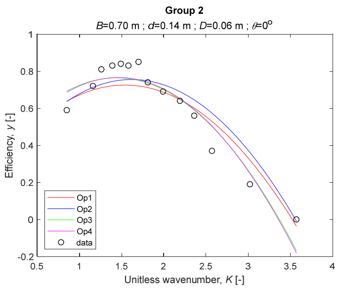
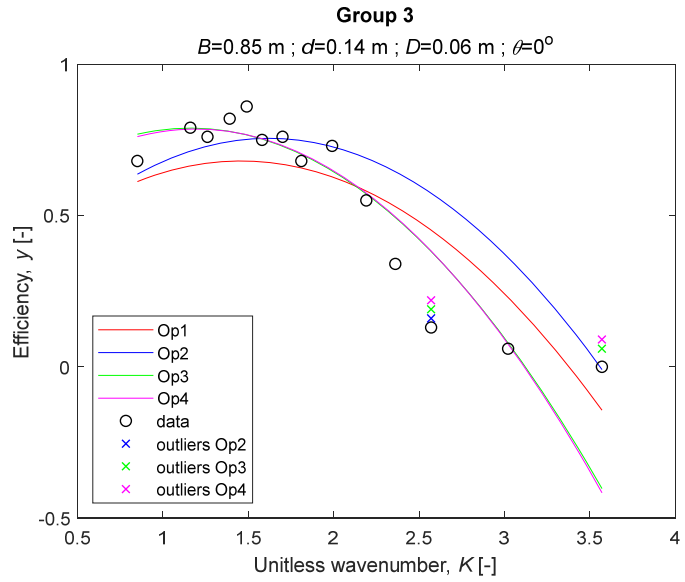
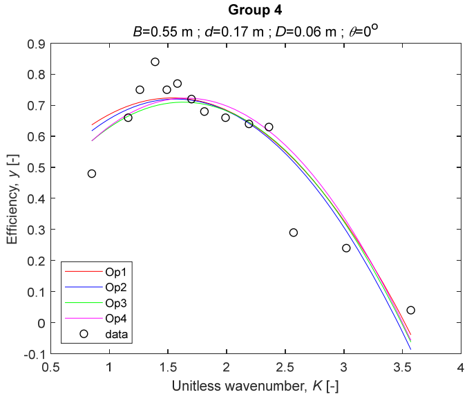
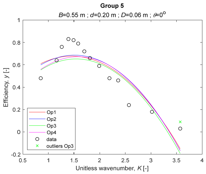
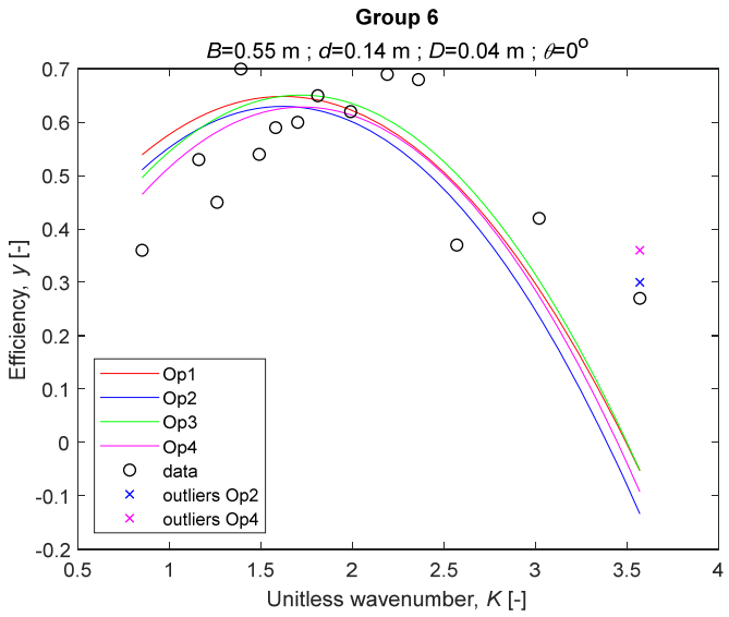
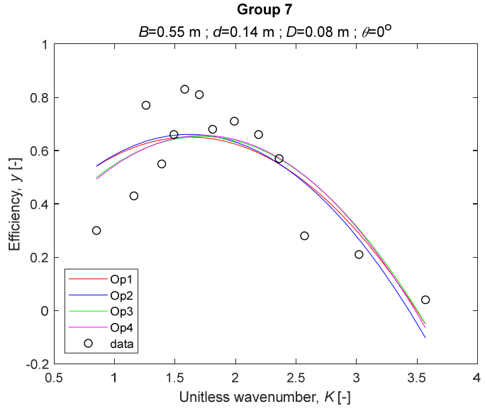
The performance measures of the developed MLR models (51)–(54) are summarized in Table 3. The graphical results of the models developed under the four outlier detection options (Op1–Op4) were presented in Figure 3, Figure 4, Figure 5, Figure 6, Figure 7, Figure 8, Figure 9, Figure 10 and Figure 11 for each of the nine experimental groups of 14 records in the training set (as described in Section 2). Only the unitless wavelength (x1 = K) is changing within any of the groups, so the MLR was depicted as nine one-dimensional graphs. We can conclude the following:
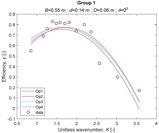
Figure 3.
The four models for Group 1.
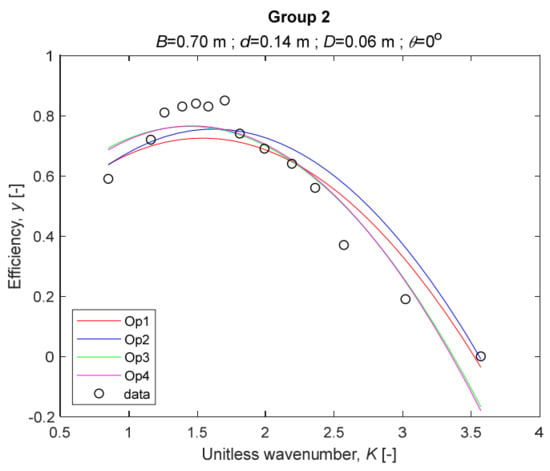
Figure 4.
The four models for Group 2.
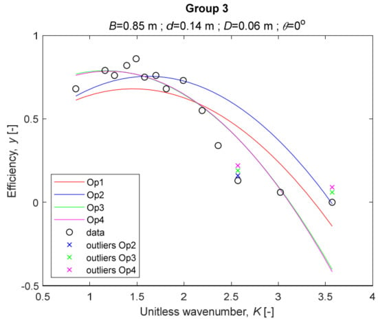
Figure 5.
The four models for Group 3. The outliers for a model are denoted above the point with a cross in a respective color.
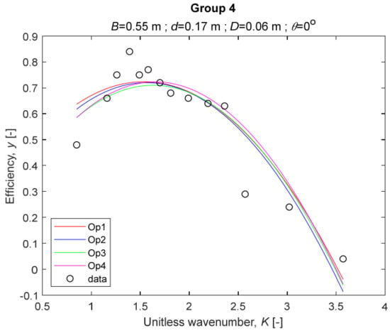
Figure 6.
The four models for Group 4.
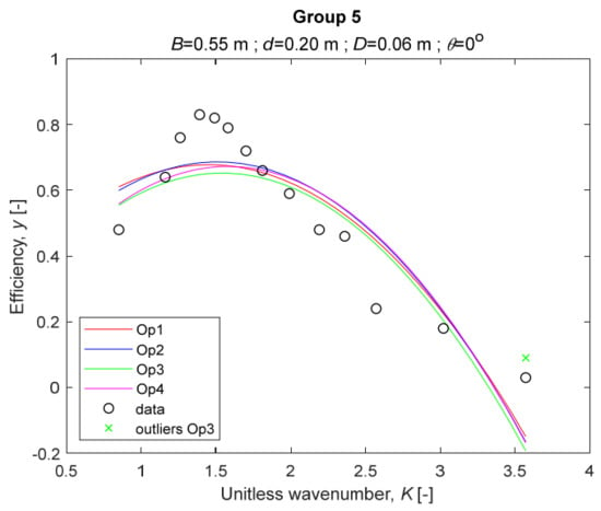
Figure 7.
The four models for Group 5. The outliers for a model are denoted above the point with a cross in a respective color.
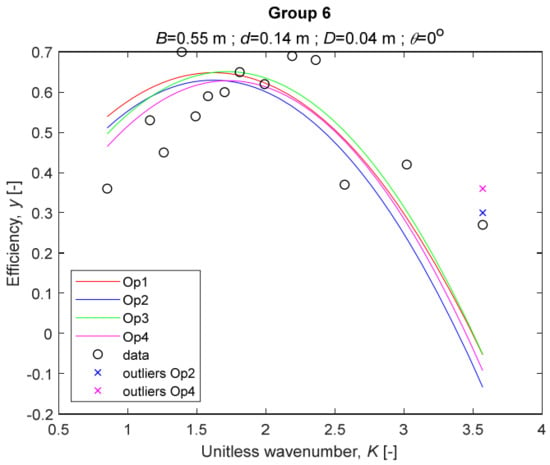
Figure 8.
The four models for Group 6. The outliers for a model are denoted above the point with a cross in a respective color.
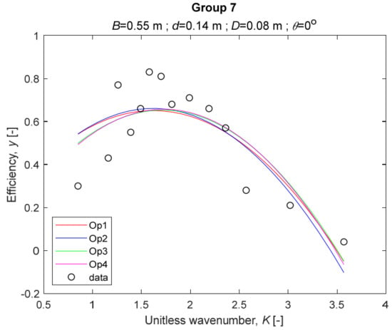
Figure 9.
The four models for Group 7.
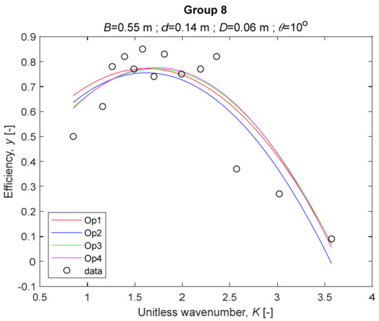
Figure 10.
The four models for Group 8.
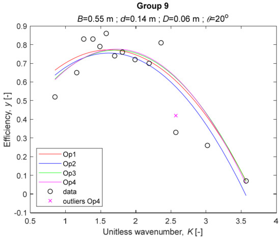
Figure 11.
The four models for Group 9. The outliers for a model are denoted above the point with a cross in a respective color.
1. The experimental data given in Figure 3, Figure 4, Figure 5, Figure 6, Figure 7, Figure 8, Figure 9, Figure 10 and Figure 11 contain no obvious pattern of hydrodynamic efficiency (y) dependency on the unitless wavenumber (x1 = K) even for the experiments in a single group. That shows that the problem of hydrodynamic efficiency prediction of OWC WEC is far from trivial.
2. Neither of the four developed models includes a regressor, which depends on the slope of the bottom, xi,5 = θ. That result supports the one reported in [34], but contradicts the predictions of the analytical model in [15]. Additional experimental work is needed to produce a training data set with a more balanced and diverse slope of the bottom values.
3. The four developed models use regressors depending on the unitless wavenumber (x1 = K), on the width of the chamber (x3 = B), and on the diameter of the orifice (x4 = D). All developed models, except the model (52) developed under Op2, include one or two regressors that depend on the submerged front wall length (x2 = d). Such a result is expected and shows that the stepwise regression algorithm, MSRA, has performed excellently in four setups determined by Op1, Op2, Op3, and Op4.
4. The holdout performance measures, based on the predicted residuals, were quite satisfactory for all of the four regressions (see Table 3) which proves the credibility of the developed MLR models for hydrodynamic efficiency prediction of OWC WEC. Figure 3, Figure 4, Figure 5, Figure 6, Figure 7, Figure 8, Figure 9, Figure 10 and Figure 11 show that the data has high levels of inherited variability with low signal-to-noise ratio (SNR). We can see that the very elaborate model presented in [33] produced predictions not much better than ours because of the inherited variability. Even if a model fits all data points in its prediction, it is because the model reflects not the signal, but the noise in the data, which is a well-known problem of overfitting and a recipe for disaster in engineering. Very often, in engineering practice we consider models with R2 below 0.8 to be poorly specified. This assumption is not absolute but depends on the inherited variability in the data. Furthermore, R2 is an optimistic measure of performance, and it is better to be replaced by . Even though there is no adopted practice for the , the high values of (from 0.730 to 0.787) are particularly impressive. Figure 3, Figure 4, Figure 5, Figure 6, Figure 7, Figure 8, Figure 9, Figure 10 and Figure 11 also show the lack of bias, which shows that most likely there are no missing variables in the models. Having in mind that those models would be utilized in the preliminary design, where their simplicity is as important as precision, the four developed models are rather useful.
5. Only five records from the training set have been identified as outliers: one observation (40) from all the three models, two observations (42 and 84) from two models each, and two observations (70 and 124) from a single model each. This (combined with the first conclusion) shows that the applied outlier detection algorithm, CODPA, produced conservative and consistent results under three different setups (Op2, Op3, and Op4).
6. The developed MLR models (51)–(54) are very similar which is demonstrated by the closeness of the four curves in each of the nine Figure 3, Figure 4, Figure 5, Figure 6, Figure 7, Figure 8, Figure 9, Figure 10 and Figure 11. The fact proves that the MLR models produce robust and reliable predictions when constructed properly by testing and relaxing the classical assumption of the CNLRM.
7. Taken on face value, model (54) has the best performance measures, followed on almost equal distances by the models (53), (52), and (51). However, the first model rejected four observations, the second rejected three, the third rejected two, and the last rejected none of the observations. It seems that the marginal improvement in performance measures under the different options are due to the slightly increased outlier rejection rate in Op4 compared to the other options. Another consideration in the classification of the four options is that Op4 is computationally most expensive, followed by Op3 and Op2 which are equally computationally expensive, and Op1 is the computationally cheapest options. All these considerations point out that there is no clear winner from the four models. Additional research activities are needed to determine the right place of the CODPA in the process of assumption’s diagnostics in linear regression models. It is not impossible to consider that the answer is problem specific and/or more than one option should be used consistently to achieve robust outlier rejection.
5. Conclusions
An achievement of the paper is that we developed a cost and time effective MLR model, which is very useful in the preliminary stages of design of WECs. Our model utilized an existing experimental data set to reliably predict the hydrodynamic efficiency of an oscillating water column (OWC) with satisfactory accuracy. The reliability of the model is mostly due to the novel assumptions of the diagnostic algorithms that were proposed and applied in the described case study. More specifically, our work introduced several new/modified procedures, based mainly on predicted residuals and SVD:
(1) PCCSV (Algorithm 1) is a novel procedure for reliable identification of the zero singular values of any matrix.
(2) MSRA (Algorithm 2) is a modified algorithm for stepwise regression execution in three phases with balanced treatment of the constant term. It explicitly applies the improved SVD decomposition procedure and implicitly uses the predicted residuals (by utilizing t-tests with robust HC3 estimator of the parameters covariance matrix, which is based on predicted residuals).
(3) MHTRA (Algorithm 3) is a modified algorithm which deals with the heteroskedasticity by constructing better auxiliary regression and identifies practically insignificant heteroscedasticity in the original model. It explicitly applies the improved SVD decomposition procedure three times and it explicitly uses predicted residuals several times.
(4) We proposed a novel test of the validity of the nullity assumption based on predicted residuals.
(5) We modified the Jarque–Bera test for error normality where the p-value is derived by a Monte-Carlo procedure (Algorithm 4). It explicitly applies predicted residuals.
(6) We developed and investigated the performance of four options for the placement of the applied outlier procedure CODPA (also using predicted residuals) in the overall diagnostic sequence and although the results were inconclusive, the different algorithms produced surprisingly stable predictions of the hydrodynamic efficiency of the OWC WEC devices.
As a future development, we will concentrate on four different research directions. The first one is to apply the developed procedure on several new data sets to clarify the questions with dubious answers in the present paper. The second direction is to improve continuously the proposed algorithms. One possibility could be to develop more precisely the WLS model in MHTRA. Another possibility is to try improving MSRA by utilizing t-tests with the promising robust HC4 estimator of the parameters’ covariance matrix, as advocated in [42]. The third direction of future research is to modify the presented algorithms to deal with time series problems instead of only problems with cross-sectional data. That is a challenging task because in such problems the correlation assumption must be tested and relaxed with a cutting-edge procedure. Additionally, the right place of such a procedure in the overall diagnostic sequence needs empirical justification which is by no means trivial as the question for the proper placement of the applied outlier procedure CODPA will be readdressed. The fourth one refers to the application area of our procedures. The OWC device we selected was an illustrative example for the newly developed MLR procedures. However, the developed models produced promising hydrodynamic performance results. In future studies, we will attempt to apply the methodology to other types of WEC, such as absorbers, overtopping devices, etc.
Author Contributions
Conceptualization, K.T. and N.N.; methodology, K.T. and N.A.; software, K.T. and N.N.; validation, N.A. and H.A.; investigation, N.A. and H.A.; data curation, N.A. and H.A.; writing— original draft, N.N. and N.A.; writing—review and editing, K.T. and N.N.; visualization, K.T. All authors have read and agreed to the published version of the manuscript.
Funding
This research received no external funding.
Institutional Review Board Statement
Not applicable.
Informed Consent Statement
Not applicable.
Conflicts of Interest
The authors declare no conflict of interest.
References
- Jin, J.; Hyun, B.; Liu, Z.; Hong, K. Numerical prediction of chamber performance for OWC wave energy converter. J. Korean Soc. Mar. Env. Energ. 2010, 13, 91–98. [Google Scholar]
- Benreguig, P.; Pakrashi, V.; Murphy, J. Assessment of primary energy conversion of a closed-circuit OWC wave energy converter. Energies 2019, 12, 1962. [Google Scholar] [CrossRef]
- Luo, Y.; Wang, Z.; Peng, G.; Xiao, Y.; Zhai, L.; Liu, X.; Zhang, Q. Numerical simulation of a heave-only floating OWC (oscillating water column) device. Energy 2014, 76, 799–806. [Google Scholar] [CrossRef]
- Fleming, A.; Penesis, I.; Goldsworthy, L.; Macfarlane, G.; Bose, N.; Denniss, T. Phase averaged flow analysis in an oscillating water column wave energy converter. J. Offshore Mech. Arct. Eng. 2013, 135, 021901-1–021901-9. [Google Scholar] [CrossRef]
- Stratigaki, V.; Troch, P.; Stallard, T.; Forehand, D.; Kofoed, J.; Folley, M.; Benoit, M.; Babarit, A.; Kirkegaard, J. Wave Basin Experiments with Large Wave Energy Converter Arrays to Study Interactions between the Converters and Effects on Other Users in the Sea and the Coastal Area. Energies 2014, 7, 701–734. [Google Scholar] [CrossRef]
- Ásgeirsson, G.S. Hydrodynamic Investigation of Wave Power Buoys. Master’s Thesis, Kungliga Teknishka Hogskolan, Stockholm, Sweden, 2013. [Google Scholar]
- Banks, M.; Abdussamie, N. The response of a semisubmersible model under focused wave groups: Experimental investigation. J. Ocean Eng. Sci. 2017, 2, 161–171. [Google Scholar] [CrossRef]
- ITTC (International Towing Tank Conference), Recommended Procedures and Guidelines: Wave Energy Converter-Model Test Experiments (7.5-02-07-03.7), Specialist Committee on Testing of Marine Renewable Devices of the 28th ITTC, 1-17, 2017.
- Stratigaki, V.; Troch, P.; Stallard, T.; Kofoed, J.P.; Benoit, M.; Mattarollo, G.; Babarit, A.; Forehand, D.; Folley, M. Large scale experiments on farms of heaving buoys to investigate wake dimensions, near-field and far-field effects. In Proceedings of the 33rd International Conference on Coastal Engineering, Santander, Spain, 1–6 July 2012; Volume 1(33), pp. 71–77. [Google Scholar]
- López, I.; Iglesias, G. Efficiency of OWC wave energy converters: A virtual laboratory. Appl. Ocean Res. 2014, 44, 63–70. [Google Scholar] [CrossRef]
- Teixeira, P.; Davyt, D.; Didier, E.; Ramalhais, R. Numerical simulation of an oscillating water column device using a code based on Navier-Stokes equations. Energy 2013, 61, 513–530. [Google Scholar] [CrossRef]
- Elhanafi, A.; Fleming, A.; Macfarlane, G.; Leong, Z. Numerical hydrodynamic analysis of an offshore stationary–floating oscillating water column–wave energy converter using CFD. Int. J. Nav. Archit. Ocean Eng. 2017, 9, 77–99. [Google Scholar] [CrossRef]
- Zhang, Y.; Zou, Q.; Greaves, D. Air-water two-phase flow modelling of hydrodynamic performance of an oscillating water column device. Renew. Energy 2012, 41, 159–170. [Google Scholar] [CrossRef]
- Thorimbert, Y.; Latt, J.; Cappietti, L.; Chopard, B. Virtual wave flume and Oscillating Water Column modeled by lattice Boltzmann method and comparison with experimental data. Int. J. Mar. Energy 2016, 14, 41–51. [Google Scholar] [CrossRef]
- Ning, D.; Shi, J.; Zou, Q.; Teng, B. Investigation of hydrodynamic performance of an OWC (oscillating water column) wave energy device using a fully nonlinear HOBEM (higher-order boundary element method). Energy 2015, 83, 177–188. [Google Scholar] [CrossRef]
- Evans, D. Wave-power absorption by systems of oscillating surface pressure distributions. J. Fluid Mech. 1982, 114, 481–499. [Google Scholar] [CrossRef]
- Morris-Thomas, M.; Irvin, R.; Thiagarajan, K. An investigation into the hydrodynamic efficiency of an oscillating water column. J. Offshore Mech. Arct. Eng. 2007, 129, 273–278. [Google Scholar] [CrossRef]
- Amarkarthik, A.; Sivakumar, K. Investigation on modeling of non-buoyant body typed point absorbing wave energy converter using Adaptive Network-based Fuzzy Inference System. Int. J. Mar. Energy 2016, 13, 157–168. [Google Scholar] [CrossRef]
- Abdussamie, N.; Ojeda, R.; Daboos, M. ANFIS method for ultimate strength prediction of unstiffened plates with pitting, corrosion. Ships Offshore Struct. 2018, 13, 540–550. [Google Scholar] [CrossRef]
- Zadeh, L. Is there a need for fuzzy logic? Inf. Sci. 2008, 178, 2751–2779. [Google Scholar] [CrossRef]
- Diaz-Curbelo, A.; Andrade, R.A.E.; Municio, A.M.G. The Role of Fuzzy Logic to Dealing with Epistemic Uncertainty in Supply Chain Risk Assessment: Review Standpoints. Int. J. Fuzzy Syst. 2020, 22, 2769–2791. [Google Scholar] [CrossRef]
- Coppi, R. Management of uncertainty in statistical reasoning: The case of regression analysis. Internat. J. Approx. Reason. 2008, 47, 284–305. [Google Scholar] [CrossRef]
- Pinkus, A. Approximation theory of the MLP model in neural networks. Acta Numer. 1999, 8, 143–195. [Google Scholar] [CrossRef]
- Ok, D.; Pu, Y.; Incecik, A. Artificial neural networks and their application to assessment of ultimate strength of plates with pitting corrosion. Ocean Eng. 2007, 34, 2222–2230. [Google Scholar] [CrossRef]
- Jain, P.; Deo, M. Neural networks in ocean engineering. Ships Offshore Struct. 2006, 1, 25–35. [Google Scholar] [CrossRef]
- Amundarain, M.; Alberdi, M.; Garrido, A.; Garrido, I. Neural rotational speed control for wave energy converters. Int. J. Control. 2011, 84, 293–309. [Google Scholar] [CrossRef]
- Ludwig, O.; Nunes, U.; Araujo, R. Eigenvalue decay: A new method for neural network regularization. Neurocomputing 2014, 124, 33–42. [Google Scholar] [CrossRef]
- Paneiro, G.; Rafael, M. Artificial neural network with a cross-validation approach to blast-induced ground vibration prop-agation modeling. Undergr. Space 2020. [Google Scholar] [CrossRef]
- Kang, X.; Liu, X.; Li, J.; Zhao, Y.; Zhang, H. Heat Capacity Prediction of Ionic Liquid Based on Quantum Chemistry Descriptors. Ind. Eng. Chem. Res. 2018, 57, 16989–16994. [Google Scholar] [CrossRef]
- Zhao, Y.; Zeng, S.; Huang, Y.; Afzal, R.M.; Zhang, X. Estimation of heat capacity of ionic liquids using S σ-profile molecular descriptors. Ind. Eng. Chem. Res. 2015, 54, 12987–12992. [Google Scholar] [CrossRef]
- Farahani, N.; Gharagheizi, F.; Mirkhani, S.A.; Tumba, K. A simple correlation for prediction of heat capacities of ionic liquids. Fluid Phase Equilib. 2013, 337, 73–82. [Google Scholar] [CrossRef]
- Zhao, Y.; Huang, Y.; Zhang, X.; Zhang, S. Prediction of Heat Capacity of Ionic Liquids Based on COSMO-RS Sσ-Profile. Comput. Aided Chem. Eng. 2015, 37, 251–256. [Google Scholar]
- Ning, D.; Wang, R.; Zou, Q.; Teng, B. An experimental investigation of hydrodynamics of a fixed OWC Wave Energy Converter. Appl. Energy 2016, 168, 636–648. [Google Scholar] [CrossRef]
- Abdussamie, N.; Ham, M.; Ojeda, R.; Penesis, I. Cost and time effective prediction technique for OWC-WEC devices. In Proceedings of the 28th International Ocean and Polar Engineering Conference, Sapporo, Japan, 10–15 June 2018; pp. 649–656. [Google Scholar]
- Brun, M.; Xu, Q.; Dougherty, E. Which is better: Holdout or full-sample classifier design? J. Bioinform. Syst. Biol. 2008, 2007, 297945. [Google Scholar] [CrossRef] [PubMed]
- Maddala, G. Introduction to Econometrics; Macmillan Publishing Company: New York, NY, USA, 1988; pp. 117–118, 162–163, 411–412. [Google Scholar]
- Selvanathan, E.; Selvanathan, S.; Keller, G. Business Statistics, 8th ed.; Cengage Learning: Southbank, Australia, 2021; pp. 791, 801, 878. [Google Scholar]
- Lind, D.; Marchal, W.; Wathen, S. Statistical Techniques in Business & Economics, 15th ed.; McGraw-Hill Irwin: New York, NY, USA, 2012; pp. 531–533. [Google Scholar]
- Gujarati, D. Basic Econometrics, 4th ed.; Tata McGraw Hill: New York, NY, USA, 2004; pp. 148–149, 378, 947–948. [Google Scholar]
- King, G.; Roberts., M. How robust standard errors expose methodological problems they do not fix, and what to do about it. Polit. Anal. 2015, 23, 159–179. [Google Scholar] [CrossRef]
- Wooldridge, J.; Wadud, M.; Lye, J.; Jayeux, R. Introductory Econometrics, 2nd Asia-Pacific ed.; Cengage Learning: Southbank, Australia, 2021; pp. 333–335, 358–360. [Google Scholar]
- Cribari-Neto, F. Asymptotic inference under heteroskedasticity of unknown form. Comput. Stat. Data Anal. 2004, 45, 215–233. [Google Scholar] [CrossRef]
- MacKinnon, J.; White, H. Some heteroskedasticity-consistent covariance matrix estimators with improved finite sample properties. J. Econ. 1985, 29, 305–325. [Google Scholar] [CrossRef]
- Press, W.; Teukolski, S.; Vetterling, W.; Flannery, B. Numerical Recipes—The Art of Scientific Computing, 3rd ed.; Cambridge University Press: Cambridge, NY, USA, 2007; pp. 788–798. [Google Scholar]
- Nikolova, N.; Rodriguez, R.; Symes, M.; Toneva, D.; Kolev, K.; Tenekedjiev, K. Outlier detection algorithms over fuzzy data with weighted least squares. Int. J. Fuzzy Syst. 2021. in print. [Google Scholar]
- James, G. Modern Engineering Mathematics; Pearson International: London, UK, 2015; p. 765. [Google Scholar]
- Baissa, D.; Rainey, C. When BLUE is not best: Non-normal errors and the linear model. Polit. Sci. Res. Methods 2020, 8, 136–148. [Google Scholar] [CrossRef]
- Fox, J. Applied Regression Analysis, Linear Models, and Related Methods; Sage Publications: Newbury Park, CA, USA, 1997; pp. 306–307. [Google Scholar]
- Radoinova, D.; Tenekedjiev, K.; Yordanov, Y. Stature estimation from long bone length in Bulgarians. Homo 2002, 52, 221–232. [Google Scholar] [CrossRef]
- Tenekedjiev, K.; Radoinova, D. Numerical procedures for stature estimating according to length of limb long bones in Bulgarian and Hungarian populations. Acta Morphol. Anthropol. 2001, 6, 90–97. [Google Scholar]
- White, H. A heteroskedasticity-consistent covariance matrix estimator and a direct test for heteroskedasticity. Econometrica 1980, 48, 817–838. [Google Scholar] [CrossRef]
- Dhaene, G.; Hoorelbeke, D. The information matrix test with Bootstrap-based covariance matrix estimation. Econ. Lett. 2004, 82, 341–347. [Google Scholar] [CrossRef]
- Golden, R.; Henley, S.; White, H.; Kashner, M. Generalized information matrix tests for detecting model misspecification. Econometrics 2016, 4, 46. [Google Scholar] [CrossRef]
- Hall, A. The information matrix test for the linear model. Rev. Econ. Stud. 1987, 54, 257–263. [Google Scholar] [CrossRef]
Publisher’s Note: MDPI stays neutral with regard to jurisdictional claims in published maps and institutional affiliations. |
© 2021 by the authors. Licensee MDPI, Basel, Switzerland. This article is an open access article distributed under the terms and conditions of the Creative Commons Attribution (CC BY) license (http://creativecommons.org/licenses/by/4.0/).


