Article

Application of Spatial Time Domain Reflectometry for Investigating Moisture Content Dynamics in Unsaturated Loamy Sand for Gravitational Drainage

1
Geotechnical Engineering Centre, School of Civil Engineering, University of Queensland, St. Lucia QLD 4072 Brisbane, Australia
2
School of Engineering, Westlake University, Hangzhou 310024, China
3
Institute of Advanced Technology, Westlake Institute for Advanced Study, Hangzhou 310024, China
4
Science-Engineering-Measurement, Sceme.de GmbH, Horn-Bad Meinberg, Amtsgericht Lemgo HRB 7181, Germany
*
Author to whom correspondence should be addressed.
Appl. Sci. 2021, 11(7), 2994; https://doi.org/10.3390/app11072994
Submission received: 28 January 2021 / Revised: 26 February 2021 / Accepted: 23 March 2021 / Published: 26 March 2021
(This article belongs to the Special Issue Trends and Prospects in Geotechnics)

Abstract

:
The strength of unsaturated soil is defined by the soil water retention behavior and soil suction acting inside the soil matrix. In order to obtain the suction and moisture profile in the vadose zone, specific measuring techniques are needed. Time domain reflectometry (TDR) conventionally measures moisture at individual points only. Therefore, spatial time domain reflectometry (spatial TDR) was developed for characterizing the moisture content profile along the unsaturated soil strata. This paper introduces an experimental set-up used for measuring dynamic moisture profiles with high spatial and temporal resolution. The moisture measurement method is based on inverse modeling the telegraph equation with a capacitance model of soil/sensor environment using an optimization technique. With the addition of point-wise soil suction measurement using tensiometers, the soil water retention curve (SWRC) can be derived in the transient flow condition instead of the static or steady-state condition usually applied for conventional testing methodologies. The experiment was successfully set up and conducted with thorough validations to demonstrate the functionalities in terms of detecting dynamic moisture profiles, dynamic soil suction, and outflow seepage flux under transient flow condition. Furthermore, some TDR measurements are presented with a discussion referring to the inverse analysis of TDR traces for extracting the dielectric properties of soil. The detected static SWRC is finally compared to the static SWRC measured by the conventional method. The preliminary outcomes underpin the success of applying the spatial TDR technique and also demonstrate several advantages of this platform for investigating the unsaturated soil seepage issue under transient flow conditions.

1. Introduction

In nature, the vadose zone above the water table can be several meters high. In this zone, the moisture stored in the soil matrix does not fill the pores completely. This form of water is no longer in positive potential but negative, as it presents a capillary tensile interaction that binds the soil particles [1]. This binding interaction thus enhances the mechanical properties of unsaturated soil, resulting in less deformation [1,2] and higher shear strength [3,4] compared to saturated soil, where water molecules encounter a compressive interaction [5]. Unsaturated soil mechanical behavior is, therefore, dependent on environmental conditions, which enhance or alleviate this binding effect, such as evapotranspiration and draining or flooding and intensive rainfall [1,2,6]. On the other hand, due to the air invasion into the soil matrix to form such a capillary water meniscus, the amount of effective hydraulic conductive channels is reduced as well and this degradation of geo-gas and groundwater flow conduits in unsaturated soil are highly concerning for the investigation of solute transport in the vadose zone [6]. For quantifying the contribution of capillary effects as water protentional in energy form and moisture content to the hydro-mechanical properties of unsaturated soil, the soil suction profile and soil moisture content profile need to be determined in order to characterize the soil water retention curve (SWRC), which is the core unsaturated soil constitutive relationship between the soil suction and moisture content (gravimetric/volumetric) [2].
The measurement of SWRC can be conducted either in the laboratory or in the field. In the laboratory, the standard axis translation technique (ATT) is often implemented [1]. Briefly, there is a one-dimensional representative elementary volume (REV) scaled soil specimen placed in a small fluid leakage-free chamber; through adding air pressure on top of the specimen, soil moisture can be expelled out of the soil matrix; the suction is the difference between applied air on top and water pressure at the bottom; the water moisture variation can be determined by measuring the mass of specimen or volume of water expelled out. Although ATT can be implemented in the laboratory due to the small set-up, this technique can only measure the SWRC under the static condition, for which there is no further moisture redistribution and capillary non-equilibrium. In the field, SWRC is usually given by separately measuring the suction profile using tensiometers and the moisture profile using in-situ sampling soil for the oven-drying method [7]. Compared to the ATT technique on a laboratory scale, this approach is more labor-expensive. In addition, sampling of soil disturbs the original configuration of the soil strata further, inducing moisture reconfiguration. This phenomenon is inevitable for in situ measurement and leads to potential falsification. Due to these limitations, there is always disagreement between the SWRC measured using ATT and in situ methods. Moreover, neither approach is able to measure the SWRC under the transient flow condition due to the requirement of equilibrium achievement and sampling procedure. Therefore, even for a homogeneous soil specimen, the conventional methods constrain the understanding of the spatial effect on soil suction determination [8,9], the temporal effect on moisture reconfiguration [10] and the dynamic effect in SWRC [11,12,13]. To overcome these limitations, there is a strong need for a laboratory experiment maintaining the homogeneity of a specimen in a full-scale soil profile without uncontrollable environmental conditions.
For measuring the SWRC under the transient flow condition, the spatially distributed moisture content needs to be measured with high temporal resolution. Some previous literature has implemented the soil column experiment using point-wise moisture sensors and tensiometers for logging the transient response of soil moisture and suction [12,14,15,16]. Nevertheless, these series of experiments only studied the dynamic effect of moisture and suction in a short sand column of less than 1 m, and this did not cover the entire suction profile of sandy soil (approximately 0–2 m). Even though these dynamic SWRC studies allow the quantification of suction and moisture under the transient flow condition, they are not able to provide information on global suction/moisture profiles due to the smaller experimental scale. To collect information on both global suction and moisture profiles, the experimental set-up should be large enough to cover the sandy soil suction profile, and the moisture content profile should also be logged within a smaller time step as well. Therefore, the spatial time domain reflectometry (spatial TDR) developed by the Soil Moisture Group (SMG) at the University of Karlsruhe [17,18,19] was applied to the experimental studies of the non-uniqueness of the SWRC on a sand column experiment and levee model [13,20]. However, in these previous experimental investigations, a high air entry (HAE) ceramic disk, having higher hydraulic resistivity than sand, was placed under the specimen to build up the hydraulic connectivity between the hanging column reservoir and specimen. This might also result in alleviation of moisture seepage velocity and, additionally, reduce the significance of the dynamic response of suction and moisture redistribution.
With the aim of mitigating the shortcomings of these previous soil column tests, a novel experimental platform is developed in this study. In this experimental platform, the spatial TDR sensors are installed in sand columns to measure the TDR waveforms consistently during one-step gravitational drainage experiments. Taking advantage of this valuable moisture measuring technique, the moisture profile along a 240-cm sand column can be calculated using an inverse modeling method developed by SMG [17,18,19]. With this powerful inverse technique, and by consistently logging TDR traces along the soil strata, a dynamic moisture profile with high spatial and temporal resolution can be achieved. With the addition of temporal logging of soil suction using a tensiometer along different elevations of the soil column, it is able to determine not only the point-wise SWRC at varied elevations but also the global suction/moisture profile under transient flow conditions. In this study, this novel laboratory-scale experimental set-up is presented. Furthermore, some preliminary outcomes of the gravitational drainage test are presented to demonstrate the capabilities of this experimental platform and eventually compared to the conventional hanging column method with discussions.

2. Spatial Time Domain Reflectometry

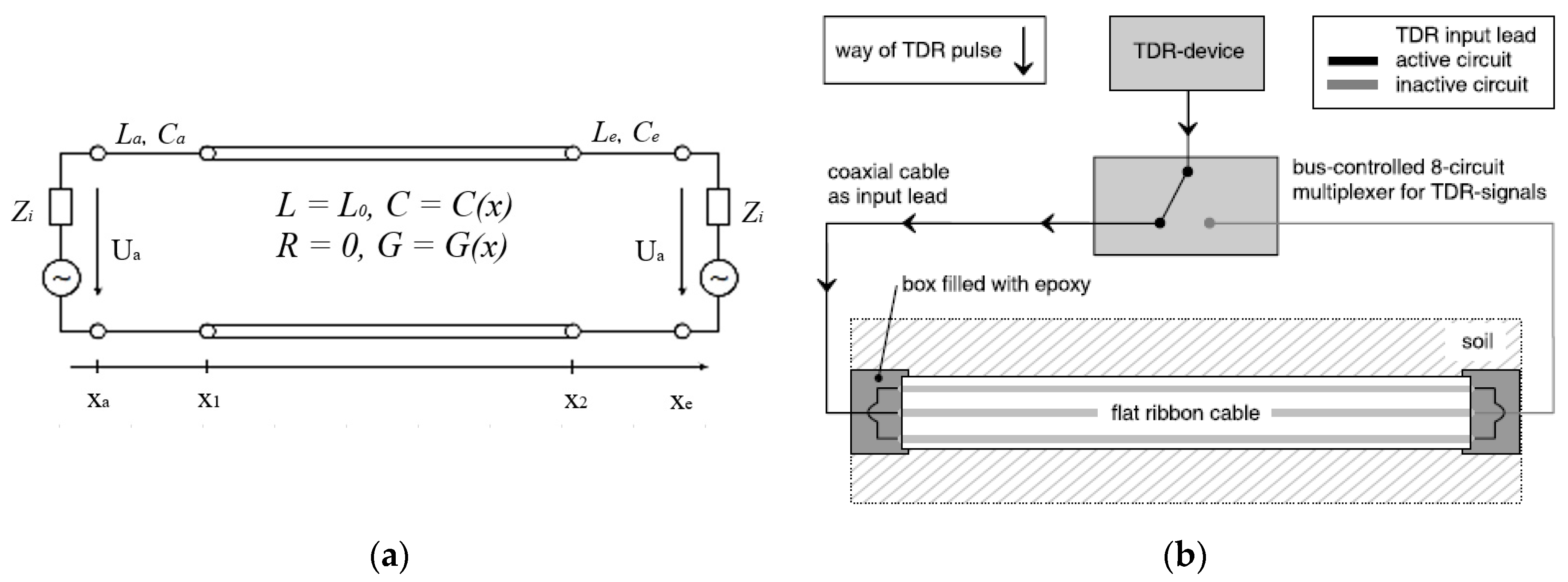
2.1. Basic Principles of Time Domain Reflectometry

Time domain reflectometry (TDR) has become an important monitoring technique for various civil engineering problems [21,22,23,24]; the main application is the monitoring of moisture content for porous media [25,26,27,28]. A TDR measurement system is composed of a pulse generator combined with an oscilloscope and a transmission line system (see Figure 1a). The transmission line includes a leading coaxial cable and a sensing waveguide, called the TDR probe, which is embedded in the medium for characterization. The characteristics (length and geometry) of the probe depend on the application. The classical geometry remains in the rod configuration. The pulse generator delivers an electromagnetic pulse along the transmission line, and the oscilloscope records returning reflection. Reflection will occur at any impedance discontinuities along the transmission line. In particular, the pulse will be reflected at the beginning and end of the TDR probes. The travel time analysis between these two reflections can be used to determine the flight time Δt of the pulse to travel along the probe. This flight time is generally computed based on the dual tangent method [29], where the reflection arrival is located at the intersection of the two tangents to the TDR curve (see Figure 1b). Finally, the apparent permittivity εapp of the medium can be determined with the well-known relation:
ε a p p = ( c 0 Δ t 2 L p ) 2
where c0 is the speed of the light and Lp is the length of the probe. Please note that for most porous media, the permittivity is complex and frequency-dependent (dispersion). The term apparent permittivity is used here because the time-domain method does not intend to compute the complete frequency-dependent complex permittivity.
In a second step, the apparent permittivity is linked to the parameter of interest—in most cases, water content, ϴ. The most frequent method is to use the empirical equation. The classical example is the famous Topp equation [30]:
θ T o p p = 5.3 × 10 2 + 2.92 × 10 2 ε a p p 5.5 × 10 4 ε a p p 2 + 4.3 × 10 6 ε a p p 3
The accuracy of such an empirical model highly depends on the nature of the soil related to density, the salinity of soil water, mineral composition, etc. For example, Topp’s equation is not suitable for high swelling clay mineral [31]. An alternative to this solution is to derive a material-specific calibration functions [32].
Another approach relies on a physical model based on mixture equations [33,34]. Mixing models consider the soil as a medium that is composed of different phases. The relative permittivity of the mixture εm is the result of the sum of the dielectric properties of each phase multiplied by its volume fraction:
ε m a = k = 1 N V k . ε r , k a
where N is the number of phases, a is a structure parameter, Vk is the volume fraction and εr,k is the relative permittivity of the solid phase. The classical configuration for the mixture equation is the three-phase mixtures (air–solid–liquid) with a structure index equal to 0.5, called the Complex Reflective Index Model (CRIM) [35]. In this configuration, εm can be expressed directly as a function of water content [36]. The main source of interest of such models is the versatility: they can take into account the temperature and frequency dependence of the single components. The main disadvantage of such a method is the lack of knowledge and understanding of the interaction between single components.

2.2. Spatial Time Domain Reflectometry Sensor Development

For the purpose of measuring natural porous media on a large scale, conventional TDR has its limitations, especially concerning the measurement of spatially distributed moisture, as probes are usually constructed as small three-pin or two-pin probes, which can only give a point measurement. Spatial TDR was developed by SMG at the Karlsruher Institute of Technology (KIT), Karlsruhe, Germany, to enable moisture profile measurements [17,18,19,37]. A flat ribbon cable consisting of three-line copper wire covered with polyethylene insulation is usually used for this purpose. An example of the spatial TDR sensor is given in Figure 2a. The corresponding conceptual model of the electrical circuit of a TDR transmission line and capacitance model are separately shown in Figure 2b,c. The electrical circuit of an infinitesimal section along the cable can be treated as the electrical circuit plotted in Figure 2b. The electrical design of the sensor was developed by Huebner, C. et al. [18].
For such a infinitesimal section, information on the surrounding soil and coating material properties can be extracted from the conductance (G) and capacitance (C) using inverse modeling of the telegraph equation [19,38,39,40,41]. For instance, one version developed by Schlaeger [5] is selected to conduct the inverse analysis in this study. Before inverse modeling, some assumptions and set-up conditions have to be achieved:
  • The resistance is assumed to be constant at a value of zero for lower frequencies (<104 Hz), because, in practical cases, dielectric losses are much higher than resistance losses, with the exception of long sensors buried into a nearly lossless material such as snow [18];
  • The inductance is assumed to be constant (L0) for lower frequencies (<104 Hz), because only the external inductance remains at the highest frequency (106~109 Hz), and a transition frequency around 100 kHz ensures the insignificant influence of the inductance increase at a low-frequency range within the time window of TDR measurement [18];
  • The conductance and capacitance depend on the surrounding moist sandy soil and are assumed to be independent of frequency for lower frequencies (<105 Hz) [17];
  • The performance of the flat ribbon cable sensor is very sensitive to the installation in accordance with the 3-D electromagnetic modeling analysis [37] because the air-filled gap of 0.25 mm on both sides of the flat ribbon cable causes significant underestimation of moisture content, while a water-filled gap leads to overestimation [17,36].

2.3. Spatial Time Domain Reflectometry Forward Modeling

Based on the above assumptions and ideal sensor installation conditions, the inverse technique on two-way TDR tracing to extract C and G profiles can be executed. According to the electrical circuit simplified in Figure 3a, the forward modeling telegraph equation can predict the TDR trace along a flat ribbon cable. Therefore, the finite difference method is applied to numerically solve these equations with boundary conditions exactly matching the physical sensor design to predict the TDR trace [38,40,41,42]. To simplify the original telegraph equations for solving, Schlaeger transformed two first-order governing partial differential equations (PDE) into a single PDE in second-order as Equation (4):
[ L C ( x ) 2 t 2 + L G ( x ) t + L / x L x 2 x 2 ] U i ( x , t ) = 0
where L is inductance, assumed to be constant because of the second assumption; C and G are, separately, capacitance and conductance in functions of cable length x because of the third assumption; U is the voltage predicted for plotting the TDR trace (i = 1,2 represents first and second TDR tracing); the resistance R is assumed to be zero because of the first assumption depicted in Figure 3a. The appropriate initial and boundary conditions for solving Equation (4) to replicate the TDR trace have been discussed in Schlaeger’s forward modeling work in detail [42]. Due to the requirement of two unknown input state variables (C and G profiles), two-way TDR tracing has to be implemented using a TDR device combined with a multiplexer, as described in Figure 3b [18,19]. The TDR device should send voltage steps through one channel of the multiplexer and then should be immediately switched to the second channel to collect the TDR waveform from the other terminal. Thus, through solving Equation (4) twice to match the two TDR waveforms collected from both terminals, the two unknown input profiles can be determined. Moreover, the forward modeling domain is constrained within two sensor terminals corresponding to two inflection points along a single TDR waveform [17].

2.4. Spatial Time Domain Reflectometry Two-Way Inverse Analysis

To extract the C and G profiles, the last step is the application of the optimization technique for minimizing the difference between forward modeling and TDR measurement results. Generally, for an optimization problem, the objective function is usually the square difference between prediction and measurement, starting from an initial estimation and finally determining with the global minimum. Schlaeger [19] derived the objective function as Equation (5):
F ( C , G ) = i = 1 2 0 T [ U i M ( x i , t , C , G ) U i m ( x i , t ) ] 2 d t
where F is the objective function of C and G; UiM and Uim are, individually, the predicted and measured voltage (i = 1,2 corresponds to two-way TDR tracing). This function has been successfully optimized using the conjugate gradient method with the reconstruction of C and G by Schlaeger [19]. The optimization procedure is to input one initial estimation of the C and G profiles into forward modeling to calculate the cost function and update the input by previous minimization outcomes until the cost function achieves the global minimum. The derivation of the Jacobin gradient of the objective function using the adjoint PDE of Equation (4) can be sourced from the mathematical study [19].

2.5. Spatial Time Domain Reflectometry One-Way Inverse Analysis

On the other hand, for the only reconstruction of the capacitance profile using one-way TDR tracing, Becker and Schlaeger [43] applied an empirical equation between C and G proposed by Håkansson [44]:
G ( C ) = { G ( 1 e C 0 C C d )   if   C C 0 0   if   0 C C 0
where G and C are the conductance and the capacitance of soil and sensor isolation, C0 and Cd are the fitting parameters for capacitance; and G is the fitting parameter for the conductance. Using Equation (6), the inverse analysis only solves one TDR trace measured from each terminal, because the capacitance profile is the only unknown input in need of optimization. This relationship was successfully used for the three-pin probe sensor in the previous study of technique development [43]. In this study, the values of fitting parameters are C0 = 50 pF/m, Cd = 40 pF/m and G = 90 mS/m.

2.6. Spatial Time Domain Reflectometry Post-Analysis

Once the capacitance profile can be inversely determined using this algorithm, the permittivity profile of the surrounding soil along the sensor can be calculated in accordance with the capacitance model characterizing the cable sensor, as shown in Figure 2c. Before calculating the permittivity of the soil (εm), the three capacitance values C1, C2 and C3 ought to be experimentally calibrated. This calibration has been completed previously (see [17,18]), and the permittivity is calculated based on the capacitance model shown in Figure 2c as:
C ( ε m ) = ε m C 1 C 2 ε m C 1 + C 2 + C 3
where C1 (14.8 pF/m), C2 (323 pF/m) and C3 (3.4 pF/m) are parameters of the capacitance model, C is the total capacitance of the soil and coating isolation, εm is relative permittivity [17]. Eventually, the soil moisture profile can be calculated by the empirical models (Equation (2)) or the phase-mixing model (Equation (3)), which needs specific calibration using a Vector Network Analyzer (VNA) with the open-ended coaxial cell [45,46,47].
Instead of the reconstruction of the capacitance profile along the sensor, the travel time determined using the tangent method along one TDR trace can also be used to calculate the mean capacitance using:
C ( ε m ) = 1 L ( t 2 L p ) 2
where C is the total capacitance for the entire measuring zone, εm is relative permittivity, L is inductance (constant L0 = 756 nH/m), t is travel time and Lp is the length of the sensor. Equation (8) is useful to validate the mean moisture content for the total measuring volume. The mean moisture content later can be determined using Equation (8) for soil permittivity with Topp’s model for the moisture content calculation.

3. Experimental Set-Up for Investigation of Soil Water Retention Behavior

The experimental set-up mainly consists of three logging systems separately recording point-wise soil suction profile, moisture content profile and accumulative outflow. An overview of the experimental platform is shown in Figure 4a, which demonstrates the view of the experimental set-up in the Geomechanics Laboratory at Geotechnical Engineering Centre, School of Civil Engineering, University of Queensland, St. Lucia QLD, Australia.

3.1. Soil Sample Specification

Two types of sandy soil were involved in this experimental set-up. One is the beach sand collected from Bribe Island, and the other one is the Budget Brickies loamy sand collected from an unknown construction site, Queensland, Australia. The particle size of the two types of sand ranges from 0.075 to 2 mm. The D50 of beach sand is 0.35 mm, which is slightly larger than the mean size of loam, 0.27 mm. The sieving analysis was implemented for both types of sand in accordance with ASTM standards of particle analysis for coarser soil [48].
The mineralogy of the two samples comprised of quartz at the specific gravity of 2.65. The coefficients of uniformity (Cu) for beach sand and loamy sand are 1.71 and 2.39 separately, and the coefficients of gradation (Cc) are 0.99 and 1.11. Based on the Unified Soil Classification System (USCS), both of them are poorly graded uniform sand (SP). The beach sand is medium sand without any fine content, while the loamy sand is fine sand with a fine content of 5%. The loamy sand is adopted for a demonstration of the results collected by the experimental platform in this study.

3.2. Moisture Profile Logging System Set-Up

As previously mentioned, the spatial TDR technique was applied to soil moisture profile measurement; four flat ribbon cable sensors were individually inserted into the centers of four empty acrylic columns (diameter = 14.35 cm and length = 240 cm). The bottom terminal of spatial TDR is fixed with an artificial gravel filter designed based on published criteria [49]. The falling head test was conducted on the gravel filter to confirm that the hydraulic conductivity of the filter (6.5 × 10⁻³~9.5 × 10⁻³ cm/s) was larger than the hydraulic conductivity of the soil specimen in the column (2.9 × 10⁻³~5.6 × 10⁻³ cm/s). It does not only indicate the end of spatial TDR but is also a highly pervious porous media under the specimen being tested. Moreover, there was no sand or fine gravel flushed out during the soil water drainage process.
Each flat ribbon cable sensor had two terminals, demanding two channels on the multiplexer. Due to the need for four sensors for four columns, a TDR trace logging system consisting of a Campbell Scientific SDM X50 multiplexer© (8-channels) combined with both a TDR100© and a CR1000 data logger© was built to connect to eight connectors of four sensors. The data logging program coded in CRBasic© was then applied for automatically logging eight TDR traces from 8 multiplexer channels to complete one/two-way TDR tracing in each soil column. An overview of the experimental set-up and illustration are separately shown in Figure 4a,b.
This technique and logging system have been successfully applied to soil column tests and embankment water content dynamics measurement [17,20]. According to previous performance measurements [17], spatial TDR can achieve a spatial resolution of 3 cm with an average deviation of around ±2% for moisture content. The TDR100© can only impulse into the single sensor by changing the single switch along eight multiplexer channels. Therefore, for two-way TDR tracing on each sensor, there has to be at least a one-second delay between the two occurrences of TDR pulsing. However, this is much smaller than the moisture redistribution speed in natural sand. Hence, this delay is neglected, and two-way TDR tracing could be seen as simultaneously implemented.
As a gravel filter designed based on filter design criteria [49] guarantees the lowest hydraulic resistivity impacts from the column bottom without internal erosion, the transient flow conditions in the measuring range will not encounter any artificial alleviation of flow velocity. Similar soil column experiments have been implemented by many previous studies [8,9,16,20,50,51,52,53]. With the exception of the 2-m soil column test [51], most of them, conducted in shorter soil columns of less than 1.2 m, required a hanging column method with a water table below the bottom of the specimen. In this case, there has to be a high air entry (HAE) porous media under the specimen to build up the hydraulic connectivity between the specimen and water reservoir for suction control. To avoid air penetrating through the HAE disk to subsequently disconnect the suction-applying reservoir from the system, such disks or membranes must possess a smaller pore size distribution (PSD), which is much smaller than the specimen. Usually, the HAE disks are ceramic disks made of clay particles sintered together. Thus, the hydraulic conductivity of the HAE material is much lower than the sandy soil specimen. It is somehow inevitable to generate a quasi-steady-state flow condition using a shorter soil column test with the adoption of an HAE disk. Additionally, such smaller column tests only allow the measurement of half of the suction and moisture profile. In this experiment, due to the use of a 2.4-m-long column with a gravel filter fixing the spatial TDR sensor to the column bottom, there was an opportunity to neglect those artificial constraints in previous experimental set-ups. On the other hand, the previous 2-m soil column test applied the oven-drying method for determining the segments of the soil column only after equilibrium was achieved [51]. In comparison to the previous study, the current experimental set-up in this study can provide moisture measurement with a high temporal and spatial resolution by applying the spatial TDR technique. These advantages demonstrate the novelties of this experimental platform.

3.3. Suction Profile Logging System Set-Up

There were five UMS T5 tensiometers© (Figure 5a) inserted into the unsaturated zone at the elevations of 40, 60, 100, 140, 180 cm, where all were the above constant water pressure head of 36 ± 1 cm, as shown in Figure 4b. Moreover, there is another tensiometer inserted into the saturated zone under the water table at the elevation of 20 cm, which is not specified in Figure 4b. There is a spatial resolution of 20 cm for suction profile logging at the column bottom in order to detect the dynamic pore water pressure around the capillary fringe area for the future investigation of SWRC dynamic effects under variable water pressure boundary conditions. In total, there are twenty-four sensors on four columns (six sensors on each column). These sensors are connected to one Geo-Datalogger (DT85G, Pacific Data©). The temporal resolution of data logging is set to 30 s. As the UMS T5 tensiometers used a Wheatstone bridge circuit (Figure 5b), according to the logger manual [54], the output value of this data logger is:
B o u t = V o u t V e x 10 6
where Bout is the dimensionless voltage, Vout is the measured bridge output voltage, Vex is the excitation voltage. In addition, the T5 sensor measuring range is from −85 KPa for suction up to +100 KPa for positive water pressure. Thus, calibration between the dimensionless voltage and water pressure was carried out for each sensor within the positive water pressure range. Due to the perfect linear equation fitting into the calibration data points in Figure 5b, the calibration equation can be applicable for the entire measurement range. Twenty-four sensors share the same slope in the linear calibration equation, except for differences in the interception (−0.2~1.5 kPa) due to the varying physical offset on each sensor. It should be noted that the physical offset depends on the maintenance of the T5 sensors. After storing them for a long period, the calibration has to be reconducted to determine the new offset values due to the aging issue of the membrane in the sensor body. When the water table drops to the hydraulic head of the constant head tank, and equilibrium is approached, the suction value can also be double-calibrated and validated by calculating the suction head above the groundwater table. Meanwhile, the trend of the dynamic response of pore pressure can also be collected under the transient flow condition. The specification of the T5 tensiometer is summarized in Table 1.
For an investigation of the soil suction profile in transient flow conditions, the response delay of the pressure sensor is of particular concern. The response time of tensiometers was fully investigated by Klute et al. [56]. For every tensiometer, there will be a time delay in the pressure response between the specimen and sensor body because of the permeability of the ceramic cup on the shaft tip. However, because the T5 sensor only measures a low suction range and the thickness of the ceramic cup is smaller than the HAE disk, there is only minor hydraulic resistance between the sensor and specimen. According to the T5 tensiometer manual [55], it only takes 5 seconds to approach an accurate value, and this is already the fastest option for suction measurement among other methods requiring moisture redistribution in a long equilibrium period, such as filter paper, dew point meters and ATT [1,2,57]. As the temporal resolution of suction logging is 30 seconds, such a small delay in response can be neglected for this experimental set-up.

3.4. Outflow Logging Set-Up, Initial and Boundary Conditions

There are four bench scales used to log accumulative outflow. As illustrated in Figure 4c, a constant head tank is attached to the output at the bottom of the column. The overflow of the constant head tank is collected by another water tank located on an electrical bench scale. In the case of evaporation leading to underestimation of outflow, every tank is covered by cling wraps with holes only for flow conduits. In Figure 4a,b, four bench scales are all connected to a USB hub with a data transmission cable between RS232 and a USB interface. In Figure 4b, one extra tank on the bench scale is located in the leftmost position with exactly the same ambient conditions to measure the water evaporation for moisture loss compensation. The maximum capacity of the bench scale (Ohaus Ranger 3000 R31P30©) is 30 kg, with a precision of ±1 g. The logging time step is also set at 30 s. On the other end of the column, cling wrap was also used to fully cover the open top of the soil column with a small pinhole to apply atmospheric pressure. The initial condition was to retain the water table. Since the valve between the constant tank and the saturated sand column was opened, the experiment was initiated. The data logging system was turned on only a few minutes before.

3.5. Specimen Installation and Operating Procedure

The density control of sand specimen installation in the column was conducted by tamping on the side of the acrylic column and vertically compacting on top of each layer. The top and bottom of each column were fixed to be exactly vertical to avoid tilting off during compaction and any inclines afterwards. In regard to minimizing the density variation along such a long column, the thickness of each soil layer was controlled to 22 ± 1 cm. With the same inner diameter of the column, it was possible to achieve a mean dry density of 1.61 ± 0.05 g/cm3 (porosity 39% ± 2%) for beach sand and 1.45 ± 0.1 g/cm3 (porosity 45% ± 4%) for loamy sand. The water used for fabricating this saturated specimen was tap water from the Geomechanics Laboratory of the University of Queensland, St. Lucia QLD, Australia, due to a lack of access to a large amount of de-aired water produced close by. However, it is non-saline water for general purpose. Under a low suction range for sand soil (0~22 kPa), soil water temperature 22 ± 1 °C and normal room temperature 23 ± 1 °C, there should be no further issue regarding nucleation, such as cavitation and boiling. The segmentation of each layer was carefully controlled to mismatch each pinhole for tensiometer insertion. A previous soil column test mentioned two approaches for tensiometer installation: installing a sensor through a pre-drilled hole or installing a sensor during the compaction process [58]. Here, the T5 sensors were all inserted into the column during the compaction process. Compared to the first method, the second ensures perfect contact between each sensor and ambient soil [58]. The gap between each sensor and pinhole was sealed with both a waterproof rubber O-ring and gas leakage-free thread tap. Each T5 sensor was originally filled with deionized water using an automatically de-aired water refilling kit, manufactured by UMS®. Except for the occurrence of the ceramic tip dried out for soil gas percolation, there will be bubble-free water in the sensor and shaft up to −101 KPa by mechanical vacuuming.
For the gravitational drainage test, the soil was oven-dried before loading into the column to avoid soil segregation carrying bubbles inside the microscale soil structure. Beach sand is completely cohesionless sand. Once the sample was oven-dried, there was no more segregation, while the loamy sand needed some crushing and mechanical shaking because of slightly cohesion. The water table was always above each layer that was being compacted for the preparation of the saturated specimen. The spatial TDR sensor was located in the center of the column, with good contact between soil and sensor, so there should be no more concerns about the failure of the spatial TDR technique because of gaps between the soil and sensor [37] and inductance variation due to distortion of the sensor geometry [17].

4. Results and Discussion

This experiment was originally designed to investigate the dynamic effects in SWRC [11], the hydraulic properties of unsaturated soil and the validity of the theories of two-phase flow in porous media for the transient flow condition [59,60,61]. Thus, this experimental platform will be used for different hydraulic boundary conditions in a sequence of the constant head, multistep in/outflow by head control. Currently, as the first stage of the constant head boundary, this experiment was conducted to assess gravitational drainage in a fully saturated sample and spontaneous imbibition to fully dry sample, which needs several months to reach equilibrium conditions without further moisture/suction variation.
However, some results regarding gravitational drainage only took a few weeks to approach equilibrium. Therefore, this part of the results is presented as a demonstration of the experimental platform’s success in this study. Comparison between this soil column test and the standard hanging column test for loamy sand is also given to depict the difference and discussion is dedicated to identifying the potential problems in the conventional testing technique. Prior to the measurement of SWRC, the spatial TDR measurement and analysis are conducted to highlight the difficulties and problems in the post-analysis of spatial TDR waveforms.

4.1. Spatial TDR Tracing during Water Table Decreasing

When this experimental platform was firstly set up, before loading the sample into the column, some previous tests were conducted to validate the signal variation of TDR traces. Thus, a pre-test was completed by dropping the water table for a single column from an originally saturated condition in order to characterize the decrease in the reflection coefficient along TDR waveforms. An illustration of this pre-test is shown in Figure 6a and the TDR traces for different water tables are shown in Figure 6b. With the water table dropping downward, the TDR traces logged from 0 to 3 min clearly show an increase in the reflection coefficient along the flat ribbon cable measured from the top. After four min, the water table is stable since no variation in the TDR waveform is visible.

4.2. Spatial TDR Waveform Variation along the Sand Column in the Drainage Test

The TDR traces for the gravitational drainage test are shown in Figure 7. Two TDR pulses are separately sent to the sensor in the column from the top and bottom. A pair of TDR traces measured from both ends of the sensor at the same time can be used to conduct the inverse analysis. According to Figure 7a (Terminal Top) and b (Terminal Bottom), it is clear that the reflection coefficient of TDR traces increases with the falling water table and water draining out of the soil column. Since air enters the pore space at the top end of the column with the dropping of the water table, TDR traces measured from the top and end show an increase in the reflection coefficient up to 0.3. Meanwhile, the second reflection points in these TDR traces, indicating the transition between the sensor and the second coaxial cable, decrease from 110 to 100 ns. The TDR traces measured from the bottom display significant changes at the end of the TDR trace, showing a more pronounced transition from the sensor to a coaxial cable (drop after the second rise in the signal). The comparison of the signals demonstrates the strong variation in the TDR traces, corresponding to the change in the moisture profile. It further proves the capability of the spatial TDR technique for characterizing information on moisture content dynamics in large-scale unsaturated soil experiments.

4.3. Validation of Spatial TDR by Outflow Logging

The measurement from the spatial TDR sensor was firstly validated by the outflow data logged using an electrical bench scale. First, the tangent method was used to determine the travel time for each TDR trace sent from the column bottom. Second, the previously determined travel time was used to calculate the total mean capacitance using Equation (8). Then, the real part of soil permittivity can be calculated using Equation (7). Finally, the volumetric moisture content is calculated by Topp’s model in Figure 8. Based on the outflow and volume of the specimen, the mean volumetric moisture content was eventually calculated and plotted in Figure 8. The moisture prediction from the spatial TDR sensor strongly agrees with the moisture content calculated from the outflow data. This demonstrates the success of electrical design with corresponding parameter calibration of the spatial TDR sensor and the applicability of Topp’s model for this loamy sand.

4.4. Inverse Analysis of Spatial TDR Trace and Dynamic Moisture Profile

Figure 9a shows the performance of optimization using one-way inverse analysis of the spatial TDR technique. By applying the optimization, the TDR traces simulated using the forward modeling telegraph equation can be well-matched with the TDR traces measured using the data logging system. Based on this acceptable fitting performance, the dynamic moisture profile can be finally calculated using Topp’s model, as shown in Figure 9b. From the beginning at 12:00 pm on 4th April, the moisture content profile was fully saturated, with a mean moisture content of around 45%. Once the one-step gravitational drainage commenced, the pore water in the upper zone drained fast in the first 8 h. After two days, by 1:56 am on 6th April, it almost achieved the equilibrium condition. The data logging from the two following days shows no significant variation in moisture profiles, indicating the final equilibrium condition achieved.
It should be noted that there is an overestimation of moisture in the capillary fringe zone because of the transition zone between the sensor and epoxy terminals. Thus, it should not be used for the determination of saturated moisture content. Instead, the saturated moisture content at the initial condition should be used to cut off the irresponsible partition to determine both the air entry value (AEV) and moisture profile in the saturated area. These series of dynamic moisture profiles demonstrate the success of inverse analysis of spatial TDR technique functioning in principle, while more effort might be required to enhance the optimization method and take consideration of frequency dependence for measuring more conductive porous media.

4.5. Validation of Pressure Measurement and Dynamic Response of Water Pressure

Figure 10a shows the good agreement between the measured suction and theoretical water pressure calculated using the hydrostatic concept at the equilibrium stage. It proves the accuracy of the previous linear calibration between value Bout and water pressure for the T5 tensiometer with the datalogger. Figure 10b gives the dynamic response of measured suction for one-step drainage for six months. In the first six hours, the water pressure sharply decreased from positive values to the negative, indicating soil suction.
A few days later, the pore water pressure still gradually dropped to equilibrium. For the rest of the six-month period, only the suction value from the tensiometer inserted at 180 cm continually decreased. This further reduction for such a long period might be due to the inevitable evaporation on the upper layer, while there were two more soil layers covered by the cling wrap over the measured zone to alleviate the impacts of subsurface evaporation. The suction logging system properly functions for this drainage test, and the dynamic behavior of negative pore pressure can be successfully recorded using this experimental platform.

4.6. Soil Water Retention Curve Measurement Compared to SWRC Using the Standard Method

Finally, the suction and moisture logging collected at equilibrium are used to plot the SWRC shown in Figure 11 in comparison to the SWRC measured by the standard hanging column method. In Figure 11, there is a slight difference in initial density between the two methods of around 2–3%. The zone of residual moisture content is around 8–9% for both methods, whereas the capillary storage (moisture content changing with soil suction) and AEV show significant differences between these two methods. Even the porosity controlled for the standard method is higher, the AEV is 1.5 kPa higher than the AEV by the large column test. In fact, the larger porosity should provide a smaller AEV.
Moreover, due to the smaller AEV achieved in the large column test, the slope of SWRC is extended, so there is rather a gradual reduction in moisture content by increasing the soil suction than the sharper wetting front measured by the standard hanging column method. Previous studies on the spatial variation in suction calculated using the height difference between a ceramic disk and water table have demonstrated the sensitivity of suction determination by varying the specimen thickness [9]. This is reconfirmed again in our experimental exploration as one of the initiative motivations of this experimental study.
However, it is still not possible to thoroughly conclude the failure or inaccuracy of using the standard method due to the insufficient repetition for constructing such a large experimental operation. Furthermore, for a non-deformable soil matrix, the initial density control determines the pore size distribution, which governs the static SWRC and AEV [63,64]. This could be also a reason for the differences. This trial still further upgrades our understanding of SWRC regarding the spatial variation in suction and moisture. There will be a higher expectation that with further repetition of the same test in the laboratory and field, with systematic control of impact factors from environmental conditions and better precision of moisture given by the inverse analysis of the spatial TDR technique, the dynamic and spatial effects of SWRC can be more comprehensively unveiled for better two-phase flow seepage simulation, unsaturated soil strength estimation and deformation prediction.

5. Summary and Reflection

The soil water retention curve (SWRC) is one of the most important constitutive relationships for the simulation of the hydraulic and mechanical behavior of unsaturated soil. As unsaturated soil effective stress, shear strength, earth pressure, consolidation and swelling are highly governed by both the soil moisture content and suction, the pre-estimation of the air–water seepage process determines the accuracy of estimating unsaturated soil’s mechanical behavior. Due to this prior importance, it is critical to comprehensively investigate the dynamic and spatial effects of soil suction and moisture redistribution because many previous studies indicate such a difference between static and dynamic measurement.
This study integrates the spatial time domain reflectometry technique, high-precision tensiometer and consistent outflow logging to investigate the dynamic response of moisture distribution, soil suction and seepage flux during a transient drainage process. As the first stage, the experimental platform has been validated by the comparison between each pair of logging systems. This demonstrates the validity and functionality of this dynamic SWRC testing platform for specific loamy sand. The preliminary result shows that this system can be applied to capture both the dynamic response and the final equilibrium stage. The SWRC measured at the final stage is compared to the SWRC using the standard hanging column method, and there is a significant difference in air entry values and capillary storage between two methods. This finding further motivates the investigation of spatial effects in suction determination regarding the flaws embedded in the conventional testing method.
On the other hand, even though this experimental set-up involves excellent techniques to consistently log three state variables, the complexity of the sensoring technique and logging system leads to difficulty regarding sufficient replication in a short period. The dynamic behavior of SWRC under draining conditions needs further analysis, and the corresponding measuring technique can still be improved in future experimental investigation. In principle, the application of the spatial TDR technique offers the researcher a higher resolution of moisture distribution varying with time, and in principle, it functions for this experimental set-up. With a great appreciation of the TDR technique development, the hydrologist and geotechnical engineer can have a better understanding of the unobservable phenomenon that is not considered in the conventional theoretical framework.

Author Contributions

Conceptualization, G.Y., Z.L. and L.L.; Data curation, T.B.; Formal analysis, G.Y. and T.B.; Investigation, Z.L., T.B. and A.S.; Methodology, T.B., A.S. and S.S.; Project administration, L.L.; Resources, T.B.; Supervision, A.S. and L.L.; Writing—original draft, G.Y.; Writing—review & editing, T.B. and A.S. All authors have read and agreed to the published version of the manuscript.

Funding

This research was funded by Linkage Project (LP120100662), from Australian Research Council. The APC was funded by the University of Queensland International Scholarship.

Institutional Review Board Statement

Not applicable.

Informed Consent Statement

Not applicable.

Data Availability Statement

Not applicable.

Acknowledgments

The first author would like to acknowledge support from the Geomechanics Laboratory of the University of Queensland, Australia and also thanks for anonymous reviewers.

Conflicts of Interest

The authors declare no conflict of interest.

References

  1. Fredlund, D.G.; Rahardjo, H. Soil Mechanics For Unsaturated Soils; John Wiley: New York, NY, USA, 1993. [Google Scholar]
  2. Lu, N.; Likos, W.J. Unsaturated Soil Mechanics; John Wiley: New York, NY, USA, 2004. [Google Scholar]
  3. Khalili, N.; Khabbaz, M. A unique relationship of chi for the determination of the shear strength of unsaturated soils. Geotechnique 1998, 48, 681–687. [Google Scholar] [CrossRef]
  4. Vanapalli, S.; Fredlund, D. Comparison of different procedures to predict unsaturated soil shear strength. Geotech. Spec. Publ. 2000, 195–209. [Google Scholar] [CrossRef] [Green Version]
  5. Terzaghi, K.; Terzaghi, K.; Engineer, C.; Czechoslowakia, A.; Terzaghi, K.; Civil, I.; Tchécoslovaquie, A.; Unis, E. Theoretical Soil Mechanics; John Wiley: New York, NY, USA, 1943; Volume 18th. [Google Scholar]
  6. Bear, J. Dynamics of fluids in porous media. Soil Sci. 1975, 120, 162–163. [Google Scholar] [CrossRef] [Green Version]
  7. ASTM D2216-10. Standard test methods for laboratory determination of water (moisture) content of soil and rock by mass. Am. Soc. Test. Mater. (ASTM) 2010. [Google Scholar] [CrossRef]
  8. Bottero, S.; Hassanizadeh, S.M.; Kleingeld, P. From local measurements to an upscaled capillary pressure–saturation curve. Transp. Porous Media 2011, 88, 271–291. [Google Scholar] [CrossRef] [Green Version]
  9. Sakaki, T.; Illangasekare, T.H. Comparison of height-averaged and point-measured capillary pressure–saturation relations for sands using a modified Tempe cell. Water Resour. Res. 2007, 43. [Google Scholar] [CrossRef]
  10. Barenblatt, G. Filtration of two nonmixing fluids in a homogeneous porous medium. Fluid Dyn. 1971, 6, 857–864. [Google Scholar] [CrossRef]
  11. Hassanizadeh, S.M.; Celia, M.A.; Dahle, H.K. Dynamic effect in the capillary pressure–saturation relationship and its impacts on unsaturated flow. Vadose Zone J. 2002, 1, 38–57. [Google Scholar] [CrossRef]
  12. Das, D.B.; Mirzaei, M. Dynamic effects in capillary pressure relationships for two-phase flow in porous media: Experiments and numerical analyses. AIChE J. 2012, 58, 3891–3903. [Google Scholar] [CrossRef] [Green Version]
  13. Scheuermann, A.; Galindo-Torres, S.; Pedroso, D.; Williams, D.; Li, L. Dynamics of water movements with reversals in unsaturated soils. In Proceedings of the 6th International Conference on Unsaturated Soils, UNSAT, Sydney, Australia, 2–4 July 2014; pp. 1053–1059. [Google Scholar]
  14. Sakaki, T.; O’Carroll, D.M.; Illangasekare, T.H. Direct quantification of dynamic effects in capillary pressure for drainage–wetting cycles. Vadose Zone J. 2010, 9, 424–437. [Google Scholar] [CrossRef]
  15. O’Carroll, D.M.; Phelan, T.J.; Abriola, L.M. Exploring dynamic effects in capillary pressure in multistep outflow experiments. Water Resour. Res. 2005, 41. [Google Scholar] [CrossRef] [Green Version]
  16. Mirzaei, M.; Das, D.B. Experimental investigation of hysteretic dynamic effect in capillary pressure–saturation relationship for two-phase flow in porous media. AIChE J. 2013, 59, 3958–3974. [Google Scholar] [CrossRef] [Green Version]
  17. Scheuermann, A.; Huebner, C.; Schlaeger, S.; Wagner, N.; Becker, R.; Bieberstein, A. Spatial time domain reflectometry and its application for the measurement of water content distributions along flat ribbon cables in a full-scale levee model. Water Resour. Res. 2009, 45. [Google Scholar] [CrossRef] [Green Version]
  18. Huebner, C.; Schlaeger, S.; Becker, R.; Scheuermann, A.; Brandelik, A.; Schaedel, W.; Schuhmann, R. Advanced measurement methods in time domain reflectometry for soil moisture determination. In Electromagnetic Aquametry; Kupfer, K., Ed.; Springer: Berlin/Heidelberg, Germany, 2005; pp. 317–347. [Google Scholar]
  19. Schlaeger, S. A fast TDR-inversion technique for the reconstruction of spatial soil moisture content. Hydrol. Earth Syst. Sci. Discuss. 2005, 9, 481–492. [Google Scholar] [CrossRef] [Green Version]
  20. Scheuermann, A.; Montenegro, H.; Bieberstein, A. Column test apparatus for the inverse estimation of soil hydraulic parameters under defined stress condition. In Unsaturated Soils: Experimental Studies; Schanz, T., Ed.; Springer: Berlin/Heidelberg, Germany, 2005; pp. 33–44. [Google Scholar]
  21. Robinson, D.; Jones, S.B.; Wraith, J.; Or, D.; Friedman, S. A review of advances in dielectric and electrical conductivity measurement in soils using time domain reflectometry. Vadose Zone J. 2003, 2, 444–475. [Google Scholar] [CrossRef]
  22. Kupfer, K.; Trinks, E.; Wagner, N.; Hübner, C. TDR measurements and simulations in high lossy bentonite materials. Meas. Sci. Technol. 2007, 18, 1118. [Google Scholar] [CrossRef]
  23. Siggins, A.; Gunning, J.; Josh, M. A hybrid waveguide cell for the dielectric properties of reservoir rocks. Meas. Sci. Technol. 2011, 22, 025702. [Google Scholar] [CrossRef]
  24. Zhang, J.; Nakhkash, M.; Huang, Y. Electromagnetic imaging of layered building materials. Meas. Sci. Technol. 2001, 12, 1147. [Google Scholar] [CrossRef]
  25. Roth, C.; Malicki, M.; Plagge, R. Empirical evaluation of the relationship between soil dielectric constant and volumetric water content as the basis for calibrating soil moisture measurements by TDR. J. Soil Sci. 1992, 43, 1–13. [Google Scholar] [CrossRef]
  26. Skierucha, W.; Wilczek, A.; Szypłowska, A.; Sławiński, C.; Lamorski, K. A TDR-based soil moisture monitoring system with simultaneous measurement of soil temperature and electrical conductivity. Sensors 2012, 12, 13545–13566. [Google Scholar] [CrossRef] [PubMed]
  27. Kaatze, U.; Hübner, C. Electromagnetic techniques for moisture content determination of materials. Meas. Sci. Technol. 2010, 21, 082001. [Google Scholar] [CrossRef]
  28. Kaatze, U. Reference liquids for the calibration of dielectric sensors and measurement instruments. Meas. Sci. Technol. 2007, 18, 967. [Google Scholar] [CrossRef]
  29. Huisman, J.; Weerts, A.; Heimovaara, T.; Bouten, W. Comparison of travel time analysis and inverse modeling for soil water content determination with time domain reflectometry. Water Resour. Res. 2002, 38, 13-1–13-8. [Google Scholar] [CrossRef]
  30. Topp, G.; Davis, J.; Annan, A.P. Electromagnetic determination of soil water content: Measurements in coaxial transmission lines. Water Resour. Res. 1980, 16, 574–582. [Google Scholar] [CrossRef] [Green Version]
  31. Kelleners, T.; Robinson, D.; Shouse, P.; Ayars, J.; Skaggs, T. Frequency dependence of the complex permittivity and its impact on dielectric sensor calibration in soils. Soil Sci. Soc. Am. J. 2005, 69, 67–76. [Google Scholar] [CrossRef]
  32. Dirksen, C.; Dasberg, S. Improved calibration of time domain reflectometry soil wate-r content measurements. Soil Sci. Soc. Am. J. 1993, 57, 660–667. [Google Scholar] [CrossRef]
  33. Sihvola, A.H. Electromagnetic Mixing Formulas and Applications; IET: Stevenage, UK, 1999. [Google Scholar]
  34. Bore, T.; Schwing, M.; Serna, M.L.; Speer, J.; Scheuermann, A.; Wagner, N. A new broadband dielectric model for simultaneous determination of water saturation and porosity. IEEE Trans. Geosci. Remote Sens. 2018, 56, 4702–4713. [Google Scholar] [CrossRef]
  35. Brovelli, A.; Cassiani, G. Effective permittivity of porous media: A critical analysis of the complex refractive index model. Geophys. Prospect. 2008, 56, 715–727. [Google Scholar] [CrossRef]
  36. Bore, T.; Wagner, N.; Delepine Lesoille, S.; Taillade, F.; Six, G.; Daout, F.; Placko, D. Error analysis of clay-rock water content estimation with broadband high-frequency electromagnetic sensors—Air gap effect. Sensors 2016, 16, 554. [Google Scholar] [CrossRef] [Green Version]
  37. Wagner, N.; Trinks, E.; Kupfer, K. Determination of the spatial TDR-sensor characteristics in strong dispersive subsoil using 3D-FEM frequency domain simulations in combination with microwave dielectric spectroscopy. Meas. Sci. Technol. 2007, 18, 1137. [Google Scholar] [CrossRef]
  38. Leidenberger, P.; Oswald, B.; Roth, K. Efficient reconstruction of dispersive dielectric profiles using time domain reflectometry (TDR). Hydrol. Earth Syst. Sci. Discuss. 2006, 10, 209–232. [Google Scholar] [CrossRef] [Green Version]
  39. Comandini, F.V.; Bore, T.; Six, G.; Sagnard, F.; Lesoille, S.D.; Moreau, G.; Placko, D.; Taillade, F. FDR for non destructive evaluation: Inspection of external post-tensioned ducts and measurement of water content in concrete. In Proceedings of the 10th International Conference on Nondestructive Evaluation (NDE) in relation to Structure Safety for Nuclear and Pressurized Components, Cannes, France, 1–3 October 2013; p. 8. [Google Scholar]
  40. Norgren, M.; He, S. An optimization approach to the frequency-domain inverse problem for a nonuniform LCRG transmission line. IEEE Trans. Microw. Theory Tech. 1996, 44, 1503–1507. [Google Scholar] [CrossRef]
  41. Lundstedt, J.; Ström, S. Simultaneous reconstruction of two parameters from the transient response of a nonuniform LCRG transmission line. J. Electromagn. Waves Appl. 1996, 10, 19–50. [Google Scholar] [CrossRef]
  42. Schlaeger, S. Inversion von TDR-Messungen zur Rekonstruktion räumlich verteilter bodenphysikalischer Parameter; Instituts für Bodenmechanik und Felsmechanik der Technischen Hochschule Fridericiana: Karlsruhe, Germany, 2002. [Google Scholar]
  43. Becker, R.; Schlaeger, S. Spatial time domain reflectometry with rod probes. In Proceedings of the 6th Conference on “Electromagnetic Wave Interaction with Water and Moist Substances”, ISEMA, Weimar, Germany, 29 May–1 June 2005. [Google Scholar]
  44. Håkansson, G. Reconstruction of Soil Moisture Profile Using Time-Domain Reflectometer Measurements. Ph.D. Thesis, Royal Institute of Technology, Stockholm, Sweden, 1997. [Google Scholar]
  45. Wagner, N.; Bore, T.; Robinet, J.C.; Coelho, D.; Taillade, F.; Delepine-Lesoille, S. Dielectric relaxation behavior of Callovo-Oxfordian clay rock: A hydraulic-mechanical-electromagnetic coupling approach. J. Geophys. Res. Solid Earth 2013, 118, 4729–4744. [Google Scholar] [CrossRef] [Green Version]
  46. Huang, Y. Design, calibration and data interpretation for a one-port large coaxial dielectric measurement cell. Meas. Sci. Technol. 2001, 12, 111. [Google Scholar] [CrossRef]
  47. Hübner, C.; Kupfer, K. Modelling of electromagnetic wave propagation along transmission lines in inhomogeneous media. Meas. Sci. Technol. 2007, 18, 1147. [Google Scholar] [CrossRef]
  48. ASTM D6913-04. Standard test methods for particle-size distribution (gradation) of soils using sieve analysis. Am. Soc. Test. Mater. (ASTM) 2009. [Google Scholar] [CrossRef]
  49. Giroud, J. Development of criteria for geotextile and granular filters. In Prestressed Geosynthetic Reinforced Soil By Compaction, Proceedings of the 9th International Conference on Geosynthetics, Guaruja, Brazil, 23–28 May 2010; IGS Brazil: Sao Paulo, Brazil, 2010; p. 4564. [Google Scholar]
  50. Rassam, D.; Williams, D. A dynamic method for determining the soil water characteristic curve for coarse-grained soils. Geotech. Test. J. 2000, 23, 67–71. [Google Scholar]
  51. Chapuis, R.P.; Masse, I.; Madinier, B.; Aubertin, M. A drainage column test for determining unsaturated properties of coarse materials. ASTM Geotech. Test J. 2007, 30, 83–89. [Google Scholar]
  52. Lins, Y.; Schanz, T.; Fredlund, D.G. Modified pressure plate apparatus and column testing device for measuring SWCC of sand. ASTM Geotech. Test J. 2009, 32. [Google Scholar] [CrossRef] [Green Version]
  53. Yan, G. Dynamic Multiphase Flow in Granular Porous Media; Faculty of Engineering, Architecture and Information and Technology (EAIT): Queensland, Australia, 2015. [Google Scholar]
  54. ThermoFisher Scientific. DT80 Range User’s Manual; Thermo Fisher Scientific Australia Pty Ltd.: Scoresby, Australia, 2013; p. 310. [Google Scholar]
  55. UMS. User Manual of T5/T5x Pressure Transducer Tensiometer; Meter Group AG: Munchen, Germany, 2009. [Google Scholar]
  56. Klute, A.; Gardner, W. Tensiometer response time. Soil Sci. 1962, 93, 204–207. [Google Scholar] [CrossRef]
  57. ASTM D6836-02. Test methods for determination of the soil water characteristic curve for desorption using a hanging column, pressure extractor, chilled mirror hygrometer, and/or centrifuge. Am. Soc. Test. Mater. (ASTM) 2003. [Google Scholar] [CrossRef]
  58. Yang, H.; Rahardjo, H.; Wibawa, B.; Leong, E.-C. A soil column apparatus for laboratory infiltration study. Geotech. Test J. 2004, 27. [Google Scholar] [CrossRef]
  59. Hassanizadeh, S.M.; Gray, W.G. Toward an improved description of the physics of two-phase flow. Adv. Water Resour. 1993, 16, 53–67. [Google Scholar] [CrossRef]
  60. Richards, L.A. Capillary conduction of liquids through porous mediums. J. Appl. Phys. 1931, 1, 318–333. [Google Scholar] [CrossRef]
  61. Kalaydjian, F.-M. Dynamic capillary pressure curve for water/oil displacement in porous media: Theory vs. experiment. In Proceedings of the SPE Annual Technical Conference and Exhibition, Washington, DC, USA, 4–7 October 1992. [Google Scholar]
  62. Yan, G.; Scheuermann, A.; Schlaeger, S.; Bore, T.; Bhuyan, H. Application of Spatial Time Domain Reflectometry for investigating moisture content dynamics in unsaturated sand. In Proceedings of the 11th International Conference on Electromagnetic Wave Interaction with Water and Moist Substances, Florence, Italy, 23–27 May 2016; p. 117. [Google Scholar]
  63. Fredlund, D.G.; Xing, A. Equations for the soil-water characteristic curve. Can. Geotech. J. 1994, 31, 521–532. [Google Scholar] [CrossRef]
  64. Zhou, A.-N.; Sheng, D.; Carter, J. Modelling the effect of initial density on soil-water characteristic curves. Geotechnique 2012, 62, 669–680. [Google Scholar] [CrossRef] [Green Version]
Figure 1. (a) Schematic description of Time Domain Reflectometry (TDR) device (pulse generator for sending a signal and oscilloscope for receiving) and TDR sensor plugged into a bulk of soil; (b) TDR waveform for saturated sand with the travel time determined by tangent method (reflection coefficient is dimensionless).
Applsci 11 02994 g001
Figure 2. (a) Flat ribbon cable used for spatial TDR measurements; (b) equivalent circuit of an infinitesimal section of cable sensor [18]; (c) capacitance model of the flat ribbon cable [17].
Applsci 11 02994 g002
Figure 3. (a) The schematic plot of spatial TDR measuring electrical circuit with previous assumptions; the flat ribbon cable is located between x1 and x2, coaxial cable is between xa and x1 or x2 and xe [19]; (b) the implementation of two-way TDR tracing using TDR device and multiplexer [17].
Applsci 11 02994 g003
Figure 4. (a) The overview of the physical experimental set-up for gravitational drainage and spontaneous imbibition experiment; (b) the specification of sensor configuration and hydraulic boundary condition for gravitational drainage experiment.
Applsci 11 02994 g004
Figure 5. (a) UMS T5 tensiometer with a 20-cm shaft (deionized water fully filled) [53]; (b) the electrical circuit of T5 tensiometer [54]; (c) the linear calibration between dimensionless voltage bout and water pressure (the red crosses are data measured for calibration using linear regression) [53].
Applsci 11 02994 g005
Figure 6. (a) The illustration of a single column drainage test without sample filled; (b) TDR waveforms indicating a drop in water table [62].
Applsci 11 02994 g006
Figure 7. TDR traces for gravitational drainage test: (a) TDR traces measured from the top; (b) TDR traces measured from the bottom [62].
Applsci 11 02994 g007
Figure 8. The mean water content dynamics for the loamy sand column in comparison with the mean water content from outflow data.
Applsci 11 02994 g008
Figure 9. (a) The fitting performance of capacitance reconstruction using one-way inversion analysis on both terminals (TDR trace sent from bottom and top); (b) the dynamic volumetric moisture content profile measured using the spatial TDR inverse analysis.
Applsci 11 02994 g009
Figure 10. (a) The comparison between tensiometer measurement and theoretical water pressure; (b) the dynamic response of tensiometer on each point.
Applsci 11 02994 g010
Figure 11. The comparison between SWRC measurements from the large soil column test (the mean ϴ averaged spatially ± 5 cm) and standard hanging column method (the data points given by the hanging column method are fitted using Fredlund and Xing (FX) model [63]).
Applsci 11 02994 g011
Table 1. Specification of UMS T5 micro-tensiometer [55].
SpecificationRange
Measuring range+100–85 kPa
Precision±0.5 kPa
Shaft diameter5 mm
Shaft length20 cm
Output signal−100 Mv + 85 mV
Publisher’s Note: MDPI stays neutral with regard to jurisdictional claims in published maps and institutional affiliations.

