Viscous Vortex Particle Method Coupling with Computational Structural Dynamics for Rotor Comprehensive Analysis

Abstract

A panel/vortex particle hybrid method is coupled with a computational structure dynamics code to predict helicopter rotor loads. The rotor blade surfaces and near wakes are modeled by the panel method, while the far wake is modeled by resorting to the vortex particles method. A fast summation method is introduced to accelerate the evolution of particle–particle-induced velocity and its derivative as well as panel–particle interactions. The developed vortex particle method code is coupled with the multibody code MBDyn to predict the rotor airloads. Numerical validations are carried, out and the results are compared with the experiments and simulation results in the literature.

1. Introduction

Rotorcrafts are characterized by strong interactions between the slender blades’ structural dynamics and the unsteady aerodynamics environment; among them, the blade vortex interaction (BVI) causes significant noise and vibration problems. These strong interactions present a substantial challenge for the prediction of airloads. A high fidelity aeroelastic simulation, coupling rotor aerodynamics with structure dynamics, is often required. Research efforts have been undertaken to develop sophisticated and comprehensive analysis methods for rotorcrafts coupling structural [1,2] and aerodynamics models [3,4]. The structural models, also referred to as “computational structural dynamics models” (CSD), perform sophisticated structural dynamics simulations by resorting to nonlinear beam models and different joints in a multibody dynamics framework and carries out the trim calculation. Several CSD codes have been developed during the past decades; among them are CAMRAD II [5], DYMORE [6], RCAS [7], UMARC [8], and MBDyn [9]. Usually, CSD codes are equipped with simplified aerodynamics models such as the lifting line model; these models are not suitable for an accurate prediction of unsteady airloads. In recent years, significant progress has been made in the use of coupled computational fluid mechanics (CFD) and CSD analysis to calculate the trim parameters and to predict the airloads and structural responses [4,10,11,12,13]. CFD methods such as Reynolds-averaged Navier–Stokes (RANS) or large-eddy simulations (LES) for rotorcraft analysis usually make use of the overset mesh methodology; provide a high-fidelity simulation; and are capable of predicting the transonic flow (shock wave) effects, separated flow, and reverse flow phenomena. However, these grid-based methods may suffer from excessive dissipation due to the numerical discretization unless a fine grid system and advanced meshing techniques such as adaptive mesh refinement (AMR) that allows us to adaptively refine the discretization around key regions of high vorticity are adopted. This makes the CFD methods more computationally expensive. Hence, a rapid assessment of aerodynamics that, at the same time, provides an acceptable fidelity may be of interest. As such, an accurate wake model is essential for rotorcraft aerodynamic models. The Lagrangian vorticity–velocity form of the incompressible Navier–Stokes equations is a natural choice in order to solve the vortex wake transport problem. The viscous vortex particle method (VPM) solves the vorticity transport equation using a grid-free Lagrangian formulation. The VPM represents the wake with a cloud of vortex particles; each particle is associated with vector-valued vorticity, velocity, and position. Based on first principles, VPM captures, without introducing any artificial numerical dissipation, the fundamental fluid flow physics for both the vorticity stretching and the physical viscous diffusion. In VPM, the aerodynamic surfaces are treated as a vorticity source that emits vortex particles into the flow field. Opoku et al. [14] modeled the far-field wake with vortex blobs, coupled with a panel method, and incorporated Fowcs Williams–Hawkings (FW–H) equation to predict the blade–vortex interaction (BVI) and aeroacoustics of a rotorcraft; however, the viscosity of the flow was not accounted for in this model. Willis et al. [15] developed the FastAero code, a fast, unsteady panel method with vortex particle wakes, and used the pre-corrected Fast Fourier Transform (FFT) approach and the fast multipole method (FMM) to accelerate the computation. Similar works have been conducted by Kenyon and Brown [16], He and Zhao [17], Tan and Wang [18] and Wang et al. [19], who combined the potential flow panel method or the lifting line model with the viscous vortex particle method. Tugnoli et al. [20] developed a flexible medium fidelity aerodynamic computational tool, called DUST, which enables different aerodynamic elements such as lifting line, vortex lattice, and vortex particles, all available in a single model. In the above works, either the fast multipole method (FMM) [21] or the Treecode method [22] were utilized to accelerate the evaluation of particle convection velocity as well as its gradient. However, when complex configurations are analyzed, the number of vortex panels increases and the computational cost from the vortex panels to the particles becomes nontrivial. For this reason, a fast summation method is required also for the vortex panels. Alvarez and Ning [23] developed a parallel viscous vortex particle method called FLOWVPM, based on the open-source code ExaFMM developed by Yokota and Barba [24] and Hu et al. [25], to evaluate the multi-rotor configuration performance. In the work of Alvarez and Ning [23], the load distribution was calculated by resorting to the blade element method (BEM) and was used to derive the circulation along the blade in order to perform all the computations using FMM, to model the lifting surfaces using embedded vortex particles, and thus to obtain an $O\left(N\right)$ simulation. However, obtaining the surface pressure of the lifting surfaces, which is of great importance for aeroacoustics analysis, is not straightforward.

In present study, a panel method is coupled with VPM. The panel method is used to model the rotor blade surfaces and near wakes, and VPM is used for far wake. Besides the classical FMM, a semi-analytical fast summation method is developed to speed up the computation of panels’ mutual interactions and of the influence exherted from the panels to the particles. The developed VPM code is coupled with the multibody code MBDyn to predict the blade unsteady aerodynamic loads. Numerical validations are carried out, and the results are compared with the experiments and simulation results in the literature.

2. Panel/Viscous Vortex Particle Aerodynamic Model

Consider the unsteady incompressible flow around the rotor configuration. According to the Helmholtz decomposition theorem, the divergence-free velocity field $\mathit{u}$ can be decomposed as $\mathit{u}={\mathit{u}}_{\infty }+{\mathit{u}}_{\varphi }+{\mathit{u}}_{\omega }$, where ${\mathit{u}}_{\infty }$ denotes the free stream field; ${\mathit{u}}_{\varphi }$ is the irrotational part induced by lifting surfaces, is defined by scalar potential $\varphi$ as ${\mathit{u}}_{\varphi }=\nabla \varphi$, and is the solution of a three dimensional boundary element method; and ${\mathit{u}}_{\omega }$ is the rotational part due to the wake, defined by a vector potential $\mathbf{\phi }$ as ${\mathit{u}}_{\omega }=\nabla \times \mathbf{\phi }$.

2.1. Panel Method

The irrotational, inviscid, incompressible potential flow is characterized by the scalar velocity potential $\varphi$, which is governed by the Laplace equation

$${\nabla }^2\varphi =0.$$

(1)

The boundary condition is derived from the requirement that the normal velocity on the boundary surface should be zero. A regularity condition at infinity is also required:

$$\frac{\partial \varphi }{\partial \mathit{n}}-{\mathit{u}}_B·\mathit{n}=0,$$

(2)

$$\underset{r\to \infty }{lim}\nabla \varphi =0.$$

(3)

The potential flow is solved by resorting to a low-order source-doublet panel method. The body surface and the wake surface are divided into quadrilateral panels with constant strength. A constant source strength on each body surface is defined as

$$\sigma =-{\mathit{u}}_B·\mathit{n},$$

(4)

where ${\mathit{u}}_B$ is the velocity of a point on a body surface and $\mathit{n}$ denotes the surface outward normal vector. Applying the internal Dirichlet boundary condition stating that the perturbed potential just inside the body surface is zero yields the linear equation system for the unknown doublets distributed on the body surface:

$$\sum _{k=1}^{N_B}{A}_k{\mu }_k=-\sum _{k=1}^{N_B}{B}_k{\sigma }_k-\sum _{k=1}^{N_W}{C}_k{\mu }_k,$$

(5)

where $A_k$, $B_k$, and $C_k$ are the potential influence coefficients of the body doublet, body source, and wake doublet, respectively, and $N_B$ and $N_W$ denote the number of body surface panels and wake surface panels, respectively. The doublets of wake panels are known from the previous time step, with the exception of those adjacent to the trailing edge, for which the doublets are determined by applying the so-called Kutta condition.

The pressure distribution on the body surface is computed from the unsteady Bernoulli equation. The nondimensionalized pressure coefficient can be calculated at any point as

$$C_p=\frac{p-p_{ref}}{MM1/2\rho V_{ref}}=1-\frac{{\left|\mathit{u}\right|}^2}{{\left|{\mathit{u}}_{ref}\right|}^2}-\frac{2}{{\left|{\mathit{u}}_{ref}\right|}^2}\frac{\partial \varphi }{\partial t},$$

(6)

where $\mathit{u}$ is the local fluid velocity and ${\mathit{u}}_{ref}$ is the local body surface velocity. The scalar velocity potential $\varphi$ is, for the current method, equal to

$$\frac{\partial \varphi }{\partial t}=-\frac{\partial \mu }{\partial t}.$$

2.2. Vortex Particle Method

It is well established that the wake has a large influence on the aerodynamics of rotorcrafts [3]. As such, an accurate wake model is essential for the rotorcraft aerodynamic model. In the present work, the wakes are modeled using the viscous vortex particle method, which is a Lagrangian formulation of the incompressible Navier–Stokes equation:

$$\frac{\mathrm{d}\mathbf{\omega }}{\mathrm{d}t}=\mathbf{\omega }·\nabla \mathit{u}+\upsilon {\nabla }^2\mathbf{\omega },$$

(7)

where $\mathbf{\omega }$ is the vorticity, $\frac{\mathrm{d}\mathbf{\omega }}{\mathrm{d}t}$ is the material derivative, and $\upsilon$ is the kinematic viscosity.

The vorticity field $\mathbf{\omega }$ is represented by N vortex particles with a vector-valued vorticity strength and by using moving Gaussian basis functions ${\xi }_{\sigma }$ as follows:

$$\mathbf{\omega }(\mathit{x},t)=\sum _{j=1}^N{\xi }_{\sigma }(\mathit{x}-{\mathit{x}}_j){\mathbf{\alpha }}_j=\sum _{j=1}^N{\xi }_{\sigma }(\mathit{x}-{\mathit{x}}_j){\mathbf{\omega }}_j{V}_j,$$

(8)

where ${\mathbf{\alpha }}_j$ is the total vorticity inside the vortex particle, ${\mathit{x}}_j$ is the location of the j th particle, $V_j$ is the particle volume, and ${\sigma }_j$ is the particle core radius. Here, ${\xi }_{\sigma }\left(\mathit{x}\right)=\xi \left(\right|\mathit{x}\left|\right)/{\sigma }^3$, and $\xi \left(\right|\mathit{x}\left|\right)$ is the Gaussian basis function that is used to smooth the vorticity field and deprecate singularity and is defined by

$$\xi \left(\right|\mathit{x}\left|\right)=\frac{1}{{\left(2\pi \right)}^{3/2}}{e}^{-{\left|\mathit{x}\right|}^2/2}.$$

(9)

With the discretized vortex particles, the viscous vorticity dynamic equation can be rewritten as follows:

$$\frac{\mathrm{d}\mathit{x}}{\mathrm{d}t}=\mathit{u},$$

(10)

$$\frac{\mathrm{d}\mathbf{\alpha }}{\mathrm{d}t}=\mathbf{\alpha }·\nabla \mathit{u}+\upsilon {\nabla }^2\mathbf{\alpha }.$$

(11)

Equation (10) describes the vortex particles convection; in Equation (11), the first term on the right hand-side is the stretching-effect term, which stands for vortex stretching and rotation due to the velocity gradient, while the second term on the right-hand side is the viscous diffusion term, which represents the vorticity diffusion caused by viscous effects. The velocity of particles can be calculated by the well-known Biot–Savart law, which is the solution to the unbounded Poisson equation:

$$\mathit{u}(\mathit{x},t)=\sum _{j=1}^N\frac{1}{{\sigma }_j^3}K\left(\rho \right)(\mathit{x}-{\mathit{x}}_j)\times {\mathbf{\alpha }}_j,$$

(12)

where $\rho =\left|\mathit{x}-{\mathit{x}}_j\right|/{\sigma }_j$ is the nondimensional distance parameter, $K\left(\rho \right)=\frac{G\left(\rho \right)-\xi \left(\rho \right)}{{\rho }^2}$ is the regularized Biot–Savart kernel for velocity evaluation, and $G\left(\rho \right)$ is the Green’s function for vector potential and can be expressed as follows:

$$G\left(\rho \right)=\frac{1}{4\pi \rho }\mathrm{erf}\left(\frac{\rho }{\sqrt{2}}\right),$$

(13)

where

$$\mathrm{erf}\left(s\right)=\frac{2}{\sqrt{\pi }}{\int }_0^s{e}^{-v^2}\mathrm{d}v$$

(14)

is the error function. The vortex particle method was shown to convergence as the number of particles increases provided that the smoothing core radius is larger than the distance between neighbor particles.

The stretching term is handled by using the so-called direct scheme, which is the dot product between the velocity gradient and the particle vorticity; the velocity gradient is obtained by analytically differentiating the velocity field, formulated as

$${\mathbf{\alpha }}_i·\nabla \mathit{u}({\mathit{x}}_i,t)=\sum _{j=1}^N\frac{1}{{\sigma }_{ij}^3}[{\mathbf{\alpha }}_j\times ]·\nabla \left[K\left(\rho \right)(\mathit{x}-{\mathit{x}}_j)\right]·{\mathbf{\alpha }}_i,$$

(15)

where ${\mathbf{\alpha }}_j\times$ is the skew symmetric matrix built from vector ${\mathbf{\alpha }}_j$. The viscous diffusion term is accounted for by using the Particle Strength Exchange (PSE) method, which approximates the Laplacian operator with an integral operator with a Gaussian kernel ${\eta }_{{\sigma }_{ij}}$, thus obtaining higher accuracy compared with numerical differentiation:

$$\upsilon {\nabla }^2{\mathbf{\alpha }}_i=\sum _{j=1}^N\frac{2\upsilon }{{\sigma }_{ij}^2}({\mathbf{\alpha }}_j{V}_i-{\mathbf{\alpha }}_i{V}_j){\eta }_{{\sigma }_{ij}}(\mathit{x}-{\mathit{x}}_j).$$

(16)

2.3. Hybrid Method

In the present method, almost all the wake panels that one would use in a normal panel method are replaced by vortex particles. At each time step, a new row of wake panels are emitted from the trailing edge, which is used to define the scalar potential jump, and their strength is determined to satisfy the Kutta condition. A second row of wake panels is generated by convecting the previous time step first row with the local velocity and by keeping their strength unchanged and is prepared to be converted into vortex particles at next time step, as depicted in Figure 1. Thus, there are always two rows of wake panels after the first time step, with the remaining portion of the wake represented by vortex particles.

The conversion of doublet wake panels to vortex particles follows Hess’s equivalence principle for which the velcocity induced at any point by a dipole with strength $\mu$ is equivalent to a surface vorticity $\gamma =\mathit{n}\times \nabla \mu$ and a boundary line vortex $\mu$. For the low-order panel method, the dipole strength is constant within each panel; thus, the surface vorticity is zero and the dipole is equivalent to a vortex ring around the perimeter of the panel. The wake panel is transformed into a vortex particle in such a way that the zero and first moments of vorticity are conserved, as illustrated in Figure 1. It is noted that, in the present work, only three edges of the wake panel are integrated into the vortex particle while the fourth edge, which is adjacent and parallel to the second row wake panels’ trailing edge, is treated as a vortex filament. The remaining vortex line can be regarded as modeling the circulation jump at the edges of the wake panel of the last row or as canceling out the circulations on the vortex particles so that Kelvin’s circulation theorem is met [15,19].

When referring to the particle velocity, the contribution from panels must be accounted for. This can be evaluated by the theory of basic singularities. Meanwhile, the stretching effect from panels to particle can be considered by differentiating the velocity field. The particles also have an influence on each panel. In a traditional source-doublet combination panel method, the particles influence is added into the freestream conditions to solve for the source strength for each panel:

$$-{\sigma }_i={\mathit{n}}_i·({\mathit{u}}_B+\sum _{j=1}^N{\mathit{u}}_{i,j}),$$

(17)

where ${\sigma }_i$ and ${\mathit{n}}_i$ are the source strength and normal vector of the ith panel, respectively, and ${\mathit{u}}_{i,j}$ is the induced velocity of particle j to panel i.

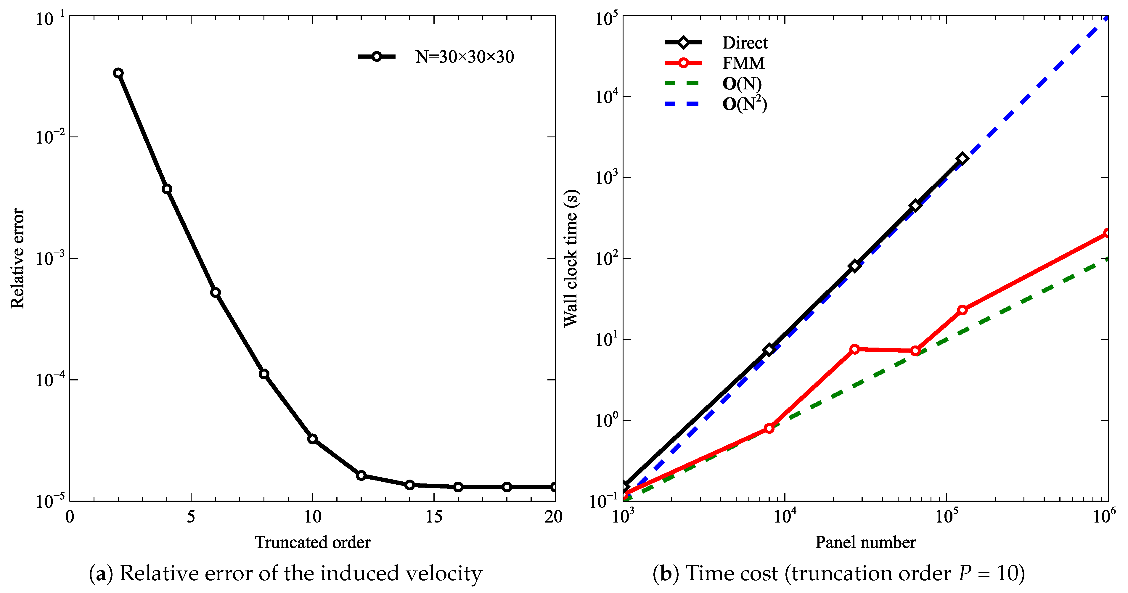
2.4. Fast Summation Method

As shown in Equation (12), calculation of the convection velocity requires, for each particle, summation over all the particles within the computation domain as well as the velocity gradient, which renders the vortex particle method a typical N-body problem with a direct summation computation complexity of $O\left(N^2\right)$ at each time step, where N is the number of particles. Two effective acceleration approaches are the TreeCode [22] and the Fast Multipole Method (FMM) [21,26], which reduce the computational complexity from $O\left(N^2\right)$ to $O(Nlog(N\left)\right)$ and $O\left(N\right)$, respectively. Both approaches utilize an Octree data structure to hierarchically subdivide the whole computation space occupied by particles into three dimensional cells and to exactly calculate the near-filed interactions by particle-to-particle (P2P) interactions while approximating the far-field interactions of the particles that are well separated. The separation threshold is defined by the Multipole Acceptance Criteria (MAC) $\frac{r_1+r_2}{R}<\theta$, where $r_1$ and $r_2$ are the radius of the source and target cell, respectively, and R is the distance between the two cells. However, FMM can approximate far-field interactions to a specified tolerance. TreeCode approximates the interaction between well-separated particles using the interactions between particle and cells by multipole expansion, which is a multipole-to-particle (M2P) interaction. In FMM, for two well-seperated cells, as depicted in Figure 2, the influence of the source cell on the center of the target cell is first calculated by a multipole-to-local (M2L) transformation, the influence can be propagated to offspring cells of the target cell by local-to-local (L2L) transformation down to the finest level, and finally the velocity of each particle in the target cell can be evaluated by accumulating the local-to-particle (L2P) interactions at the finest level.

In the present work, an adaptive Octree is built, the dual tree traversal algorithm is implemented to identify the well-separated interaction list, and the classical FMM in spherical coordinate is adopted to speed up the calculations of the convection velocity and stretching term for the particle–particle interactions. Meanwhile, as in [17] and due to the rapid decay of the kernel function, only the particles close to the target particle contribute significantly to the PSE for $\mathrm{d}{\mathbf{\alpha }}_i/\mathrm{d}t$; thus, the PSE can be considered only in the process of the particle-to-particle (P2P) interaction of FMM.

In the numerical experiments, as the rotor wake develops, the number of vortex particles increases rapidly and the vortex panel–particle interaction becomes a time-consuming computation step. A fast panel–particle evaluation is thus required as well. The velocity potential at ${\mathit{x}}_j$ generated by a constant dipole quadrilateral and source quadrilateral can be expressed as

$$\begin{array}{ccc}\hfill {\varphi }_{\sigma }& =& {\int }_S\sigma \frac{1}{|{\mathit{x}}_i-{\mathit{x}}_j|}\mathrm{d}S,\hfill \\ \hfill {\varphi }_{\mu }& =& {\int }_S\mu {\mathit{n}}_j·\nabla \left(\frac{1}{|{\mathit{x}}_i-{\mathit{x}}_j|}\right)\mathrm{d}S.\hfill \end{array}$$

(18)

Compared with the potential generated by point sources and point dipoles, one needs to compute an integral over the panel. When the target point is outside the panel, the integral is regular and can be computed accurately by a numerical method, such as a Gauss quadrature rule. When the target point is inside the panel, the integral is singular. Thus, specific approaches are needed depending on the location of the target point. In the present work, a semi-analytical method is adopted, where the inside integral is computed by resorting to an analytical method and the outside integral is evaluated by Gauss quadrature. For the inside integral, analytical expressions are available; see, e.g., [27]. When the target point is located outside the panel, as depicted in Figure 3, the integral over the quadrilateral panel is evaluated numerically. By applying the Gauss quadrature on the panel surface, Equation (18) yields

$$\begin{array}{ccc}\hfill {\varphi }_{\sigma }& =& \sum _{k=1}^K\sigma w_k\frac{1}{|{\mathit{x}}_i-{\mathit{x}}_k|},\hfill \\ \hfill {\varphi }_{\mu }& =& \sum _{k=1}^K\mu w_k\mathit{n}·\nabla \left(\frac{1}{|{\mathit{x}}_i-{\mathit{x}}_k|}\right),\hfill \end{array}$$

(19)

where ${\mathit{x}}_k$ is the Gauss quadrature point on the element; $\mathit{n}$ is the element normal vector; $\sigma$ and $\mu$ are panel source and dipole strength, respectively; and $w_k$ is a suitable integration weight. In order to compute the integration weight, the coordinates on the panel are interpolated by linear Lagrangian polynomials $N_j(\xi ,\eta )$ by $\mathit{x}(\xi ,\eta )={\sum }_j{N}_j(\xi ,\eta ){\mathit{x}}_j$, where $\xi$ and $\eta$ are the local coordinates in the local panel coordinate system and span the range $[-1,1]$. An integral ${\int }_{A}f\left(\mathit{x}\right)\mathrm{d}A$ over a quadrilateral element can thus be approximated, as customary in finite element modeling, as

$${\int }_{A}f\left(\mathit{x}\right)\mathrm{d}A={\int }_{-1}^1{\int }_{-1}^{1}f\left(\mathit{x}(\xi ,\eta )\right)∥\frac{\partial \mathit{x}}{\partial \xi }\times \frac{\partial \mathit{x}}{\partial \eta }∥\mathrm{d}\xi \mathrm{d}\eta \approx \sum _k{w}_k^{0}f\left(\mathit{x}({\xi }_i,{\eta }_i)\right){∥\frac{\partial \mathit{x}}{\partial \xi }\times \frac{\partial \mathit{x}}{\partial \eta }∥}_{|{\xi }_i,{\eta }_i},$$

(20)

where $w_k^0$ is the Gauss quadrature weight. Thus, $w_k=w_k^0{∥\frac{\partial \mathit{x}}{\partial \xi }\times \frac{\partial \mathit{x}}{\partial \eta }∥}_{|{\xi }_k,{\eta }_k}$. From Equation (19), it can be seen that the quadrilateral element can be represented by several particles located at the Gauss point and with a weighted strength. This makes it possible to implement the panel FMM into the classical particle-based fast multipole method. The multipole expansion for source and dipole quadrilateral elements can be obtained:

$$\varphi =\sum _{n=0}^P\sum _{m=n}^n{M}_n^m{r}^{-n-1}{Y}_n^m(\theta ,\varphi )$$

(21)

$$\begin{array}{ccc}\hfill {\overline{M}}_n^m& =& \sum _{k=1}^K{w}_k\sigma {\rho }_k^n{Y}_n^{-m}({\alpha }_k,{\beta }_k)\hfill \\ \hfill {\overline{\overline{M}}}_n^m& =& \sum _{k=1}^K{w}_k\mu \mathit{n}·\nabla \left({\rho }_k^n{Y}_n^{-m}({\alpha }_k,{\beta }_k)\right)\hfill \end{array}$$

(22)

where ${\overline{M}}_n^m$ and ${\overline{\overline{M}}}_n^m$ are multipole expansion coefficients for the source and dipole elements, respectively; $\rho$, $\alpha$, and $\beta$ are spherical coordinates; and $Y_n^m$ is the spherical harmonics that are consistent with those defined in Cheng et al. [26]. Compared with a standard particle, the panel itself has a finite area that could not be ignored. When constructing the Octree, some panels may belong to several boxes, making it difficult to evaluate the MAC of a panel. In the present method, the panel is firstly represented by a point located at it center, and the Octree is built with the classical procedure. After this, following a post-traversal algorithm, the box center is kept unchanged and its radius is increased in order to occupy the entire panel for the leaf box or its children box for a non-leaf box. In the modified FMM, the multipole and local expansion coefficients have 5 components: 3 for the vector-valued vorticity, 1 for the weighted dipole strength, and 1 for the weighted source strength.

A case with randomly distributed particles within a unit cubic was studied to demonstrate the convergence and acceleration of the FMM. The numerical experiments were performed on an Intel${}^{\circledR }$ Xeon${}^{\circledR }$ CPU E5-2640 0 @ 2.50 GHz desktop. Figure 4a shows the $L^2$-norm of the relative difference between the induced velocity computed by the FMM and the result computed by the analytical method. It can be seen that, when the truncation order is larger than 5, a relative error of ${10}^{-4}$ can be obtained. Figure 4b shows the time consumption of the two methods; the FMM shows its advantage for an increasing numer of particles, as expected, and when the particle number is ${10}^6$, an acceleration of over 100 times is obtained. It is clear that the computational complexity is proportional to the number of particles, $O\left(N\right)$, as it should be. In order to verify the validity of the proposed approach for the panels, the interaction of $n\times n\times n$ panels that are uniformly distributed in the unit cube was studied and the velocity measured at the center of each panel was compared with the analytical results computed with the formulae from [27]. Figure 5a shows the relative errors obtained with $30\times 30\times 30$ panels. Figure 5b reports the computational time cost and shows that a nearly linear computation complexity was obtained.

The overall speedup allowed by applying the FMM also to panels is significant for real-word simulations. As an example, the fully coupled aeroelastic simulation of the rotor of Section 5.4 takes 224 min for ten rotor revolutions if the FMM is applied to the particles alone, but the overall computational time is reduced down to 85 min after applying it also to the panels.

3. CSD Model

MBDyn is a general purpose multibody dynamics code developed at Politecnico di Milano [9]. MBDyn solves initial value problems (IVP), be them either static or dynamic. The constrained dynamics is formulated as

$$\begin{array}{ccc}\mathbf{M}\dot{\mathbf{x}}-\beta & =& \mathbf{0}\\ \dot{\beta }+{\varphi }_{/\mathbf{x}}^T{\lambda }_{\varphi }+{\psi }_{/\dot{\mathbf{x}}}^T{\lambda }_{\psi }& =& \mathbf{f}(\mathbf{x},\dot{\mathbf{x}},t)\\ \varphi (\mathbf{x},t)& =& \mathbf{0}\\ \psi (\mathbf{x},\dot{\mathbf{x}},t)& =& \mathbf{0}\end{array}$$

(23)

where $\mathbf{M}$ is the mass matrix, $\beta$ is the momentum, $\mathbf{f}$ is a vector containing generic force and moment, and ${\lambda }_{\varphi }$ and ${\lambda }_{\psi }$ are the Lagrange multipliers associated with holonomic and nonholonomic constraint equations. The differential-algebraic equation is linearized and integrated in time by using an implicit A/L stable linear multi-step integration scheme and solved by a Newton–Rapson iterative procedure.

Based on the Cosserat beam formulation, an original geometrically exact, three-node finite volume beam formulation that yields equilibrium of finite portions of beam was implemented in MBDyn as depicted in Figure 6 [28]. The internal force was computed from the nodes kinematics through the constitutive law and contributed to the equilibrium of the beam nodes. The beam cross sectional shear and warping were also accounted for by the constitutive properties of the beam cross section. The cross-sectional properties could be computed either by the variational asymptotic methods [29] or semi-analytical methods [30,31].

4. Aeroelastic Coupling

The data exchange between the aerodynamics module and structure module was accomplished by using local UNIX sockets. A loose coupling scheme was adopted. At each time step, the structure module predicts the kinematics by extrapolation and sends the predicted kinematics to the aerodynamics module; the aerodynamics module deforms the configuration based on the predicted kinematics, computes the aerodynamic forces, and sends them back to the structure module; the structure module receives the forces and iterates until convergence; and, after this, it advances to the next time step. The aeroelastic interface between the structural nodes of the beams and the aerodynamics surfaces was computed by an energy-conserving moving least-squared algorithm [32].

5. Numerical Examples

In order to validate the aerodynamic model, different helicopter rotors that have been tested by experiments under hover and forward flight condition were studied. Finally, the aerodynamic model was coupled with the CSD module and the HART II model was studied. In the present work, the rotor wake was cut off at a distance from the rotor equal to four times the rotor radius.

5.1. Caradonna–Tung Rotor

The two-bladed Caradonna–Tung rotor [33] in hover was studied here. The blade was rectangular, untwisted, and untapered and had a radius of 1.143 m and a chord of 0.1905 m. The sectional airfoil was NACA0012. The root cutoff used in simulation was equal to the chord length. The rotation speed was 1250 rpm, and the tip mach was 0.439. A total of 60 panels were arranged along the chordwise direction, with 20 panels in the spanwise direction on each blade. An azimuthal step of 5° was adopted.

In Figure 7, the predicted thrust coefficient at a collective of 5°, 8°, and 12° was compared with the experimental data. Figure 8 shows the predicted tip vortex location in both the radial direction ($r/R$) and the axis direction ($z/R$) variation as a function of the vortex age at a collective of 8°. Figure 9 shows the pressure coefficient at span locations of 50%R, 68%R, 80%R, 87%R, and 96%R. The results obtained by the present method were compared with both the experimental data and the numerical results that were obtained with a code coupling CFD and free wakes. It can be seen that good correlations exist between the present method and both the hybrid CFD method and the experiment.

5.2. AH-1G Rotor in Forward Flight

The AH-1G rotor [34] in forward flight was simulated. The rotor had two blades with the optimal load survey/tip aerodynamics and acoustics test (OLS/TAAT) airfoil. The rotor radius was equal to 6.7 m, and the blade aspect ratio was 9.8 and had a linear twist from 0° to −10° from root to tip. Each blade was modeled with 2400 panels, with 60 panels along the chordwise direction and 40 panels along the spanwise direction. The rotor was operated at an advanced ratio of 0.19, the tip mach number was equal to 0.65, and the thrust coefficient was equal to 0.00464. An azimuthal angle step of 3° was used in the present simulation.

Figure 10 and Figure 11 show the pressure coefficient at a span location equal to 60%R and 96%R and at azimuth angles of 30°, 90°, 270°, and 300°. Figure 12 illustrates the variation in the sectional thrust coefficient at span positions of 75%R, 87%R, 91%R, and 97%R over one revolution. The predicted results agree reasonably well with both the experimental data and the results computed by a CFD simulation [35]. The BVI influence on the normal force was captured by the present method on the advancing side at azimuthal angle of 50–100° and on the retreating side around an azimuthal angle of 270°.

5.3. CSD

To validate the structural model used in the present work, a clamped flexible blade, shown in Figure 13 and taken from Cheng [36], was first simulated. The results computed by the present method were compared with Dymore and with the Geometrically Exact Beam Theory (GEBT) code [37]. The blade was 1 m long and subjected to a transversal periodic force $f=10sin\left(50t\right)$ N at the free tip. Since the geometric and material properties were not provided in Cheng [36], the cross-sectional properties reported in Cheng [36] were used directly. The properties are reported in

Table 1. Beam cross-sectional properties.

Mass (kgm${}^{-1}$)	0.2	$I_{xx}$ (kgm)	10${}^{-4}$
$I_{yy}$ (kgm)	10${}^{-6}$	$I_{zz}$ (kgm)	10${}^{-4}$
$K_{11}$ (N)	10${}^6$	$K_{22}$ (N)	10${}^{20}$
$K_{33}$ (N)	10${}^{20}$	$K_{44}$ (Nm${}^2$)	50
$K_{55}$ (Nm${}^2$)	50	$K_{66}$ (Nm${}^2$)	10${}^3$

for completeness. The blade was discretized by means of 20 three-node finite volume beam elements.

Table 2. Frequency of an uncoupled blade.

GEBT	Dymore	Present
55.6 rad/s	55.6 rad/s	55.58 rad/s

lists the fundamental frequency results, and Figure 14 plots the axis displacement, transversal displacement, and flap rotation history at the blade tip. It can be seen that the current result has a good coincidence with those in Dymore and GEBT. Note that the maximum flap rotation was about 47° and that the maximum tip deflection reached about 0.5 m, 50% of the beam span. In a nutshell, the beam had definitely large rotations and deformations.

5.4. HART II Rotor Coupling with CSD

In this section, the aeroelastic simulation was validated against the experiment data from the well-known Second Higher Harmonic Control Aeroacoustic Rotor Tests (HART II) performed in the large low-speed facility of the German–Dutch Wind Tunnel (DNW) [38]. The HART-II test used a 40 percent mach scaled, four-bladed hingeless BO105 model rotor. The blades were rectangular, with a radius of 2 m, a chord of 0.121 m, a −8° linear twist, and a precone of 2.5°. The HART II tests were operated at descent conditions, where strong blade–vortex interactions (BVI) may occur. A detailed description of the experiment parameters can be found in van der Wall and Burley [39] and Smith et al. [40]; the blade properties are listed in

Table 3. HART II blade properties.

$\mathbf{Station},\mathbf{m}$	$\mathbf{x}-\mathbf{CG},\mathbf{m}$	$\mathbf{x}-\mathbf{TA},\mathbf{m}$	$\mathbf{x}-\mathbf{EA},\mathbf{m}$	$\mathbf{EA},\mathbf{N}$	${\mathbf{EI}}_{\mathit{f}},{\mathbf{Nm}}^2$	${\mathbf{EI}}_{\mathit{l}},{\mathbf{Nm}}^2$	$\mathbf{GJ},{\mathbf{Nm}}^2$	$\mathbf{Twist},°$	$\mathbf{m},\mathbf{kg}/\mathbf{m}$	${\mathbf{I}}_{\mathit{l}},\mathbf{gm}$	${\mathbf{I}}_{\mathit{f}},\mathbf{gm}$	${\mathbf{I}}_{\mathit{p}},\mathbf{gm}$
0.0	0.0	0.0	0.0	1.26 × 108	3000	14,000	380	4.24	3.67	0.4	0.4	0.8
0.075	0.0	0.0	0.0	1.26 × 108	3000	14,000	380	4.24	3.67	0.4	0.4	0.8
0.15	0.0	0.0	0.0	2.11 × 107	675	3390	380	4.24	1.57	0.29	0.052	0.342
0.19	0.0	0.0	0.0	2.11 × 107	675	4420	442	4.24	1.57	0.29	0.052	0.342
0.24	0.0006	0.0033	0.0	2.11 × 107	675	5370	500	4.24	1.72	0.41	0.052	0.462
0.29	0.0018	0.0037	−0.00195	2.05 × 107	594	5930	460	4.24	1.71	0.45	0.045	0.495
0.34	0.0019	0.0043	−0.00415	2.11 × 107	480	6610	390	4.24	1.67	0.46	0.035	0.495
0.39	0.0044	0.0073	−0.00625	1.87 × 107	400	5710	320	4.24	1.47	0.53	0.03	0.56
0.415	0.0029	0.0092	−0.00835	1.69 × 107	290	5710	280	4.24	1.45	0.69	0.024	0.714
0.44	−0.0055	0.0003	0.00535	1.17 × 107	250	5200	160	4.24	0.95	0.73	0.017	0.747
2.0	−0.0055	0.0003	0.00535	1.17 × 107	250	5200	160	−2.0	0.95	0.73	0.017	0.747

for completeness. The center of gravity (CG) and the tension axis (TA) were measured from the elastic axis (EA), while the elastic center was measured from the quarter chord; the positive direction was toward the leading edge. The inertial properties were measured with respect to the center of gravity.

Validations were performed for the baseline rotor at an advance ratio of 0.151 and a thrust coefficient equal to 0.00457. The blade was discretized by 40 finite volume beam elements, and 20 elements were placed in the blade inboard region from the hub center to $r/R=0.22$, where a significant variation in blade cross-sectional properties took place. The region from $r/R=0.22$ to tip had a constant mass distribution and structural properties and was discretized by means of 20 equally spaced beam elements. In order to model the pitching control system stiffness, as stated in [13], a torsion spring was modeled at the pitching hinge and the spring stiffness was tuned to match a non-dimensional first torsion frequency of 3.845 $/\mathrm{rev}$, which was reported in the HART II document. At first, the fan plot was predicted by the current CSD method for the HART II rotor blade to verify the structure modeling, as shown in Figure 15. The dominant natural mode shapes, i.e., the first three flap shapes, the first two lead-lag shapes, and the first torsion shape, were also compared at 100% rotational speed with those from the HART II documents [39,41] and with those computed by UMARC [42]. As seen in Figure 16, the present results correlate well with those computed by UMARC; the difference in the torsion mode at the root was due to the different boundary condition applied at the pitching hinge: in the present simulation, a lumped torsion spring was used, and this led to a twist discontinuity at the pitching hinge. In addition, as seen from Figure 15, the present model is able to predict transitions between modes of vibration. In general, the predicted mode shapes are in good agreement with those from the HART II document data.

In the simulation, each blade was modeled by $40\times 20$ panels and an azimuthal angle step of ° was used. The rotor was trimmed in order to reach the experiment thrust coefficient and zero longitudinal and lateral moments at an effective shaft tilt of 4.5° using the Newton–Raphson iterative method [35,43]. The trimmed parameters are listed in

Table 4. Trim parameters.

	Collective	Longitudinal	Lateral
Experiment	3.80$°$	−1.34$°$	1.92$°$
Present	3.925$°$	−1.116$°$	1.347$°$

.

The azimuth-wise variation for the sectional normal load $C_N{M}^2$ at the 87% span-wise location is shown in Figure 17 and is compared with the experiment results and CFD/CSD coupling results from the work of Biedron and Lee-Rausch [44] (FUN3D/CAMRAD-II), Boyd [12] (OVERFLOW2/CAMRAD-II), and Kim and Kwon [45], which couples KFLOW and a nonlinear Euler–Bernoulli beam CSD solver. The airloads show good correlation with the experimental data and the CFD/CSD results, and from the azimuthal angle of 0° to 75° at the advancing side and from 270° to 360° at the retreating side, the magnitude and location of the unsteady loading (BVI) events are well captured. $C_N{M}^2$ is computed by integrating the lower surface pressure and upper surface pressure along the chordwise direction, following the method described by Swanson et al. [46] and Johnson [47], that is

$$C_N{M}^2=\frac{N}{MM1/2\rho a^{2}c},$$

(24)

$$N={\int }_0^c{P}_L\mathrm{d}x-{\int }_0^c{P}_U\mathrm{d}x,$$

where N is the sectional normal force, a is the air speed, c is the chord length, and $P_L$ and $P_U$ are upper and lower surface pressure, respectively.

6. Conclusions

In this paper, a panel/viscous vortex particle hybrid method was developed and was coupled to the multibody dynamic code MBDyn to predict the blade unsteady aerodynamic loads. The lifting surfaces were modeled by vortex panels with constant dipole and source strength. The wake panels were shed from the trailing edge according to the Kutta conditon and were converted to viscous vortex particles as soon as they were convected downstream. The fast multipole method was utilized to accelerate the computation of the induced velocity and of its gradient. The proposed method was validated by comparison with the Caradonna–Tung rotor in hover and the AH-1G rotor in forward flight. Finally, the vortex particle code was coupled with MBDyn, and the HART II baseline model was simulated. The following conclusions can be drawn:

• When the vortex panel method was combined with the viscous vortex particle method, the predicted blade pressure, normal thrust, and wake geometry match well with experimental data and CFD results both in the hover and forward flight conditions.
• The classical particle-based fast multipole method was extended to a hybrid particle-panel computational domain by using a semi-analytical approach. The convergence of numerical tests show that, as the truncation order grows, a reasonable accuracy can be obtained; in addition, the numerical tests show that the presented algorithm has a computational complexity of $O\left(N\right)$.
• When t vortex code was coupled with the computational structural dynamics code MBDyn, the results show that the VPM/MBDyn coupling approach can predict the unsteady airloads well and is capable of capturing the BVI phenomenon, a necessary requisite for a future, accurate evaluation of the rotor aeroacoustic response.

References

1. Hodges, D.H. Review of composite rotor blade modeling. AIAA J. 1990, 28, 561–565. [Google Scholar] [CrossRef]
2. Hodges, D.H. Unified approach for accurate and efficient modeling of composite rotor blade dynamics The Alexander A. Nikolsky honorary lecture. J. Am. Helicopter Soc. 2015, 60, 1–28. [Google Scholar] [CrossRef]
3. Leishman, G.J. Principles of Helicopter Aerodynamics with CD Extra; Cambridge University Press: Cambridge, UK, 2006. [Google Scholar]
4. Datta, A.; Nixon, M.; Chopra, I. Review of rotor loads prediction with the emergence of rotorcraft CFD. J. Am. Helicopter Soc. 2007, 52, 287–317. [Google Scholar] [CrossRef] [Green Version]
5. Johnson, W. Rotorcraft Aeromechanics Applications of a Comprehensive Analysis. In Proceedings of the Heli Japan 98, AHS International Meeting on Advanced Rotorcraft Technology and Disaster Relief, Gifu, Japan, 21–23 April 1998. [Google Scholar]
6. Bauchau, O.A.; Bottasso, C.L.; Nikishkov, Y.G. Modeling rotorcraft dynamics with finite element multibody procedures. Math. Comput. Model. 2001, 33, 1113–1137. [Google Scholar] [CrossRef]
7. Saberi, H.; Khoshlahjeh, M.; Ormiston, R.A.; Rutkowski, M.J. Overview of RCAS and application to advanced rotorcraft problems. In Proceedings of the American Helicopter Society 4th Decennial Specialist’s Conference on Aeromechanics, San Francisco, CA, USA, 21–23 January 2004. [Google Scholar]
8. Bir, G.; Chopra, I.; Nguyen, K. Development of UMARC (University of Maryland advanced rotorcraft code). In Proceedings of the 46th AHS Annual National Forum, Washington, DC, USA, 21–23 May 1990. [Google Scholar]
9. Masarati, P.; Morandini, M.; Mantegazza, P. An Efficient Formulation for General-Purpose Multibody/Multiphysics Analysis. J. Comput. Nonlinear Dyn. 2014, 9, 041001. [Google Scholar] [CrossRef]
10. Bauchau, O.; Ahmad, J. Advanced CFD and CSD methods for multidisciplinary applications in rotorcraft problems. In Proceedings of the 6th Symposium on Multidisciplinary Analysis and Optimization, Bellevue, WA, USA, 4–6 September 1996; p. 4151. [Google Scholar]
11. Potsdam, M.; Yeo, H.; Johnson, W. Rotor airloads prediction using loose aerodynamic/structural coupling. J. Aircr. 2006, 43, 732–742. [Google Scholar] [CrossRef]
12. Boyd, D.D. HART-II acoustic predictions using a coupled CFD/CSD method. In Proceedings of the American Helicopter Society 65th Annual Forum, Grapevine, TX, USA, 27–29 May 2009. [Google Scholar]
13. Smith, M.J.; Lim, J.W.; van der Wall, B.G.; Baeder, J.D.; Biedron, R.T.; Boyd, D.D.; Jayaraman, B.; Jung, S.N.; Min, B.Y. The HART II international workshop: An assessment of the state of the art in CFD/CSD prediction. Ceas Aeronaut. J. 2013, 4, 345–372. [Google Scholar] [CrossRef]
14. Opoku, D.G.; Triantos, D.G.; Nitzsche, F.; Voutsinas, S.G. Rotorcraft aerodynamic and aeroacoustic modelling using vortex particle methods. In Proceedings of the 23rd International Congress of Aeronautical Sciences (ICAS 2002), Toronto, ON, Canada, 8–13 September 2002; pp. 8–13. [Google Scholar]
15. Willis, D.J.; Peraire, J.; White, J.K. A combined pFFT-multipole tree code, unsteady panel method with vortex particle wakes. Int. J. Numer. Methods Fluids 2007, 53, 1399–1422. [Google Scholar] [CrossRef]
16. Kenyon, A.R.; Brown, R.E. Wake dynamics and rotor-fuselage aerodynamic interactions. J. Am. Helicopter Soc. 2009, 54, 12003. [Google Scholar] [CrossRef] [Green Version]
17. He, C.; Zhao, J. Modeling rotor wake dynamics with viscous vortex particle method. AIAA J. 2009, 47, 902–915. [Google Scholar] [CrossRef]
18. Tan, J.F.; Wang, H.W. Simulating unsteady aerodynamics of helicopter rotor with panel/viscous vortex particle method. Aerosp. Sci. Technol. 2013, 30, 255–268. [Google Scholar] [CrossRef]
19. Wang, Y.; Abdel-Maksoud, M.; Song, B. A boundary element-vortex particle hybrid method with inviscid shedding scheme. Comput. Fluids 2018, 168, 73–86. [Google Scholar] [CrossRef]
20. Tugnoli, M.; Montagnani, D.; Fonte, F.; Zanotti, A.; Droandi, G. Mid-Fidelity Analysis of Unsteady Interactional Aerodynamics of Complex VTOL Configurations. In Proceedings of the 45th European Rotorcraft Forum, Warsaw, Poland, 17–20 September 2019. [Google Scholar]
21. Greengard, L.; Rokhlin, V. A fast algorithm for particle simulations. J. Comput. Phys. 1987, 73, 325–348. [Google Scholar] [CrossRef]
22. Barnes, J.; Hut, P. A hierarchical O (N log N) force-calculation algorithm. Nature 1986, 324, 446–449. [Google Scholar] [CrossRef]
23. Alvarez, E.J.; Ning, A. High-Fidelity Modeling of Multirotor Aerodynamic Interactions for Aircraft Design. AIAA J. 2020, 58, 4385–4400. [Google Scholar] [CrossRef]
24. Yokota, R.; Barba, L.A. FMM-based vortex method for simulation of isotropic turbulence on GPUs, compared with a spectral method. Comput. Fluids 2013, 80, 17–27. [Google Scholar] [CrossRef] [Green Version]
25. Hu, Q.; Gumerov, N.A.; Yokota, R.; Barba, L.; Duraiswami, R. Scalable fast multipole accelerated vortex methods. In Proceedings of the 2014 IEEE International Parallel & Distributed Processing Symposium Workshops, Phoenix, AZ, USA, 19–23 May 2014; pp. 966–975. [Google Scholar]
26. Cheng, H.; Greengard, L.; Rokhlin, V. A fast adaptive multipole algorithm in three dimensions. J. Comput. Phys. 1999, 155, 468–498. [Google Scholar] [CrossRef]
27. Hess, J.L.; Smith, A.O. Calculation of potential flow about arbitrary bodies. Prog. Aerosp. Sci. 1967, 8, 1–138. [Google Scholar] [CrossRef]
28. Ghiringhelli, G.L.; Masarati, P.; Mantegazza, P. Multibody Implementation of Finite Volume C Beams. AIAA J. 2000, 38, 131–138. [Google Scholar] [CrossRef]
29. Cesnik, C.E.; Hodges, D.H. VABS: A new concept for composite rotor blade cross-sectional modeling. J. Am. Helicopter Soc. 1997, 42, 27–38. [Google Scholar] [CrossRef]
30. Giavotto, V.; Borri, M.; Mantegazza, P.; Ghiringhelli, G.; Carmaschi, V.; Maffioli, G.; Mussi, F. Anisotropic beam theory and applications. Comput. Struct. 1983, 16, 403–413. [Google Scholar] [CrossRef]
31. Morandini, M.; Chierichetti, M.; Mantegazza, P. Characteristic behavior of prismatic anisotropic beam via generalized eigenvectors. Int. J. Solids Struct. 2010, 47, 1327–1337. [Google Scholar] [CrossRef] [Green Version]
32. Quaranta, G.; Masarati, P.; Mantegazza, P. A conservative mesh-free approach for fluid-structure interface problems. In Proceedings of the International Conference for Coupled Problems in Science and Engineering, Santorini Island, Greece, 25–28 May 2005. [Google Scholar]
33. Caradonna, F.X.; Tung, C. Experimental and Analytical Studies of a Model Helicopter Rotor in Hover; Technical Report TM 81232; NASA: Washington, DC, USA, 1980.
34. Cross, J.L.; Watts, M.E. Tip Aerodynamics and Acoustics Test: A Report and Data Survey; Technical Report NASA-RP-1179; NASA: Washington, DC, USA, 1988.
35. Kim, J.W.; Park, S.H.; Yu, Y.H. Euler and Navier-Stokes Simulations of Helicopter Rotor Blade in Forward Flight Using an Overlapped Grid Solver. In Proceedings of the 19th AIAA Computational Fluid Dynamics, San Antonio, TX, USA, 22–25 June 2009. [Google Scholar] [CrossRef]
36. Cheng, T. Structural Dynamics Modeling of Helicopter Blades for Computational Aeroelasticity. Ph.D. Thesis, Massachusetts Institute of Technology, Cambridge, MA, USA, 2002. [Google Scholar]
37. Hodges, D.H. A mixed variational formulation based on exact intrinsic equations for dynamics of moving beams. Int. J. Solids Struct. 1990, 26, 1253–1273. [Google Scholar] [CrossRef]
38. Yu, Y.H.; Tung, C.; van der Wall, B.; Pausder, H.J.; Burley, C.; Brooks, T.; Beaumier, P.; Delrieux, Y.; Mercker, E.; Pengel, K. The HART-II Test: Rotor Wakes and Aeroacoustics with Higher-Harmonic Pitch Control (HHC) Inputs-the Joint German/French/Dutch/US Project; Technical Report; National Aeronautics And Space Admin Langley Research Center: Hampton VA, USA, 2002.
39. van der Wall, B.G.; Burley, C.L. 2nd HHC Aeroacoustic Rotor Test (HART II)–Part II: Representative Results; Technical Report IB 111-2005/03; German Aerospace Center (DLR) Institute of Flight Systems Helicopter Division: Braunschweig, Germany, 2005. [Google Scholar]
40. Smith, M.J.; Lim, J.W.; van der Wall, B.G.; Baeder, J.D.; Biedron, R.T.; Boyd, D.D., Jr.; Jayaraman, B.; Jung, S.N.; Min, B.Y. An assessment of CFD/CSD prediction state-of-the-art using the HART II international workshop data. In Proceedings of the American Helicopter Society 68th Annual Forum, Fort Worth, TX, USA, 1–3 May 2012. [Google Scholar]
41. van der Wall, B.G. 2nd HHC Aeroacoustic Rotor Test (HART II)–Part I: Test Documentation; Technical Report IB 111-2003/31; German Aerospace Center (DLR) Institute of Flight Systems Helicopter Division: Braunschweig, Germany, 2003. [Google Scholar]
42. Kumar, A.A.; Viswamurthy, S.; Ganguli, R. Correlation of helicopter rotor aeroelastic response with HART-II wind tunnel test data. Aircr. Eng. Aerosp. Technol. 2010. [Google Scholar] [CrossRef]
43. Yang, Z.; Sankar, L.N.; Smith, M.J.; Bauchau, O. Recent improvements to a hybrid method for rotors in forward flight. J. Aircr. 2002, 39, 804–812. [Google Scholar] [CrossRef]
44. Biedron, R.; Lee-Rausch, E. Rotor airloads prediction using unstructured meshes and loose CFD/CSD coupling. In Proceedings of the 26th AIAA Applied Aerodynamics Conference, Honolulu, HI, USA, 18–21 August 2008; p. 7341. [Google Scholar]
45. Kim, Y.; Kwon, O.J. Aeroelastic Study for HART II Rotor Using Unstructured Mixed Meshes. Int. J. Aeronaut. Space Sci. 2019, 20, 1–15. [Google Scholar] [CrossRef]
46. Swanson, S.M.; McCluer, M.S.; Yamauchi, G.K.; Swanson, A.A. Airloads Measurements from a 1/4-Scale Tiltrotor Wind Tunnel Test; Technical Report; NASA Ames Research Center: Washington, DC, USA, 1999.
47. Johnson, W. Calculation of the Aerodynamic Behavior of the Tilt Rotor Aeroacoustic Model (TRAM) in the DNW; Technical Report; Army/NASA Rotorcraft Division, Army Aviation and Missile Command, Aeroflightdynamics Directorate (AMRDEC), Ames Research Center: Moffett Field, CA, USA, 2001.
Figure 1. A description of the conversion of the wake doublet panel to vortex particles.
Applsci 11 03149 g001
Figure 2. Flow of FMM calculation.
Applsci 11 03149 g002
Figure 3. Gauss quadrature diagram on the vortex panel (the red circles stand for the Gauss quadrature points).
Applsci 11 03149 g003
Figure 4. Fast multipole method (FMM) for vortex particles.
Applsci 11 03149 g004
Figure 5. FMM for vortex panels.
Applsci 11 03149 g005
Figure 6. Three-node finite volume beam.
Applsci 11 03149 g006
Figure 7. Thrust coefficient at different collective pitch angles.
Applsci 11 03149 g007
Figure 8. Tip vortex positions at a collective pitch angle of 8°.
Applsci 11 03149 g008
Figure 9. Pressure coefficients at a collective pitch angle of 8°.
Applsci 11 03149 g009aApplsci 11 03149 g009b
Figure 10. Pressure coefficient at r/R = 0.60.
Applsci 11 03149 g010
Figure 11. Pressure coefficient at r/R = 0.91.
Applsci 11 03149 g011
Figure 12. Sectional thrust for the AH-1G rotor at different radial locations.
Applsci 11 03149 g012
Figure 13. Clamped flexible blade.
Applsci 11 03149 g013
Figure 14. Tip displacement of an uncoupled flexible blade under excitation f = 10 sin ( 50 t ) at the tip.
Applsci 11 03149 g014
Figure 15. HART II rotor blade frequencies.
Applsci 11 03149 g015
Figure 16. HART II rotor blade natural mode shapes.
Applsci 11 03149 g016
Figure 17. HART II baseline case.
Applsci 11 03149 g017