Article

3D Snow Sculpture Reconstruction Based on Structured-Light 3D Vision Measurement

1
School of Instrumentation Science and Engineering, Harbin Institute of Technology, Harbin 150001, China
2
School of Mechanical and Electrical Engineering, Harbin Vocational and Technical College, Harbin 150001, China
3
College of Computer Science and Technology, Harbin Engineering University, Harbin 150001, China
4
Heilongjiang Hengxun Technology Co., Ltd., Harbin 150080, China
5
College of Electronics Science, Northeast Petroleum University, Daqing 163318, China
*
Authors to whom correspondence should be addressed.
Appl. Sci. 2021, 11(8), 3324; https://doi.org/10.3390/app11083324
Submission received: 6 January 2021 / Revised: 26 March 2021 / Accepted: 29 March 2021 / Published: 7 April 2021
(This article belongs to the Special Issue Intelligent Processing on Image and Optical Information, Volume II)

Abstract

:
Structured-light technique is an effective method for indoor 3D measurement, but it is hard to obtain ideal results outdoors because of complex illumination interference on sensors. This paper presents a 3D vision measurement method based on digital image processing to improve resistance to noise of measuring systems, which ensuresnormal operation of a structured-light sensor in the wild without changing its components, and the method is applied in 3D reconstruction of snow sculpture. During image preprocessing, an optimal weight function is designed based on noise classification and minimum entropy, and the color images are transformed into monochromatic value images to eliminate most environmental noise. Then a Decision Tree Model (DTM) in a spatial-temporal context of video sequence is used to extract and track stripe. The model is insensitive to stubborn noise and reflection in the images, and the result of the model after coordinate transformation is a 3D point cloud of the corresponding snow sculpture. In experimental results, the root mean square (RMS) error and mean error are less than 0.722 mm and 0.574 mm respectively, showing that the method can realize real-time, robust and accurate measurement under a complex illumination environment, and can therefore provide technical support for snow sculpture 3D measurement.

1. Introduction

Digitalized archive of cultural relics and artworks has become an important means for their restoration and virtual museum construction thanks to the development of 3D measurement technique. Snow sculpture is an aesthetical form of artwork peculiar to cold regions around the world in winter, as shown in Figure 1, and its cultural value is no less than painting, wood carving, architecture and other artistic expressions [1,2]. However, when warmed up, these artworks, great displays of the wisdom of their designer artists, will disappear. Snow sculpture can be divided into two categories from the perspective of creation [3]. The first category is designed and constructed according to three-dimensional computer modeling, the 3D data of which is known in advance, meaning that there is no need to measure. The other category is works improvised according to shape and texture of snow billet and combined with surrounding scenes.Similar to other sculptures, they fuse the ideas and inspirations of artists. The category of snow sculpture is unique and needs to measure and record 3D data. Therefore, both snow sculpture designers and management companies want to obtain and store 3D data of each snow sculpture in the computer, thereby making it easy to reproduce the original appearance of snow sculpture through technologies such as 3D movie and 3D printing. Obviously, there is actual demand for 3D measurement of snow sculpture and its scene reconstruction [2], but relevant research has rarely been carried out.
At present, the main methods for 3D measurement of cultural relics and artworks include laser scanning, sequence image method and structured-light vision measurement [4,5,6,7]. Laser scanning is highlyaccuratebut expensive, and its point cloud is not dense enough to adequately describe details. Sequence image method has low requirements for equipment and is easy to operate, but it cannot measure objects without obvious texture (such as pure white porcelain bottles) and has low accuracy. Structured-light vision measurement has the advantages of high accuracy, simple equipment, easy operation and low cost, but the camera is easily affected by illumination. Considering large size, single surface color, complex texture, and low cost of snow sculpture, structured-light vision measurement is more suitable for 3D measurement of snow sculpture.
Structured-light sensors need to work in a relatively controlled light environment traditionally [8], so it is usually operated in a room, while measuring outdoors has always been a challenge. However, snow sculpture is directly exposed to the outdoor environment with sunlight, shadows, reflections, and other environmental noise factors everywhere. Night scanning can reduce the noise, but it is adverse to operator’s health and work quality in the temperature range of −20 °C to −30 °C. 3D laser scanner can perform 3D measurements such as scanning ancient buildings in the day, but its sparse scanning point cloud cannot fully describe the details of snow sculpture. Therefore, we take advantage of a structured-light sensor with a laser as the light source to scan snow sculpture precisely in the field. Moreover, compared to the coding mode, which is mostly used in controlled scenes, the fixed mode structured-light sensor with better anti-noise performance [9] is more applicable for 3D measurement of snow sculpture.
It is hard to obtain a higher signal to noise ratio (SNR) even when using a laser projection outdoors, because the intensity of sunlight is usually 2–5 orders of magnitude higher than that of structured-light stripe [8]. The existing methods have not well resolved this problem. For example, Microsoft’s Kinect operates difficultly in high ambient light [10]. Modifying the structured-light sensor, such as installing filter or increasing the intensity of the light source, is a method to reduce noise, but it is at the expense of robustness and cost. So many researchers prefer to solve the above problems by digital image processing.
Stripe extraction is the key factor for fixed mode structured-light equipment to improve measurement accuracy, because the calibration and coding processes have been fixed. In Reference [8], Gupta et al. proposed an adaptive stripe intensity method to improve SNR by adjusting the width of stripe according to the intensity of sunlight, which does not increase the extra power consumption, but reduces the scanning efficiency. In Reference [11], O’Toole et al. analyzed the stripe collected by a camera on direct and indirect light projection paths, and the ambient noise was directly ignored, but the optical simulating model is too complicated. In Reference [12], Steger proposedan unbiased detection method based on Hessian matrix, which can locate the curve points in sub-pixel accuracy and has strong anti-interference ability, but it relies heavily on segmentation results of stripe area. In Reference [13], Usamentiaga et al. segmented foreground information using center of gravity method.Then the relative motion of two trapezoidal windows was used to search the laser skeleton, and curve fitting was used to mend the laser stripe gap.
All the above methods focus on eliminating noise and extracting light stripe from a single image, while few establish frame-to-frame correlation of consecutive video. Inter-frame correlation can be regarded as a process of target tracking. In the presence of environmental noise, surface reflection and partial occlusion, a combination of spatial and temporal information can be used to detect laser stripe stably and rapidly. In Reference [14], Janne used Kalman filter to track segmented light stripe, and their brightness, length, direction and position are used to establish the correlation of adjacent frames. This method is used to detect obstacles outdoors, but it is only suitable for part of outdoor scenes.
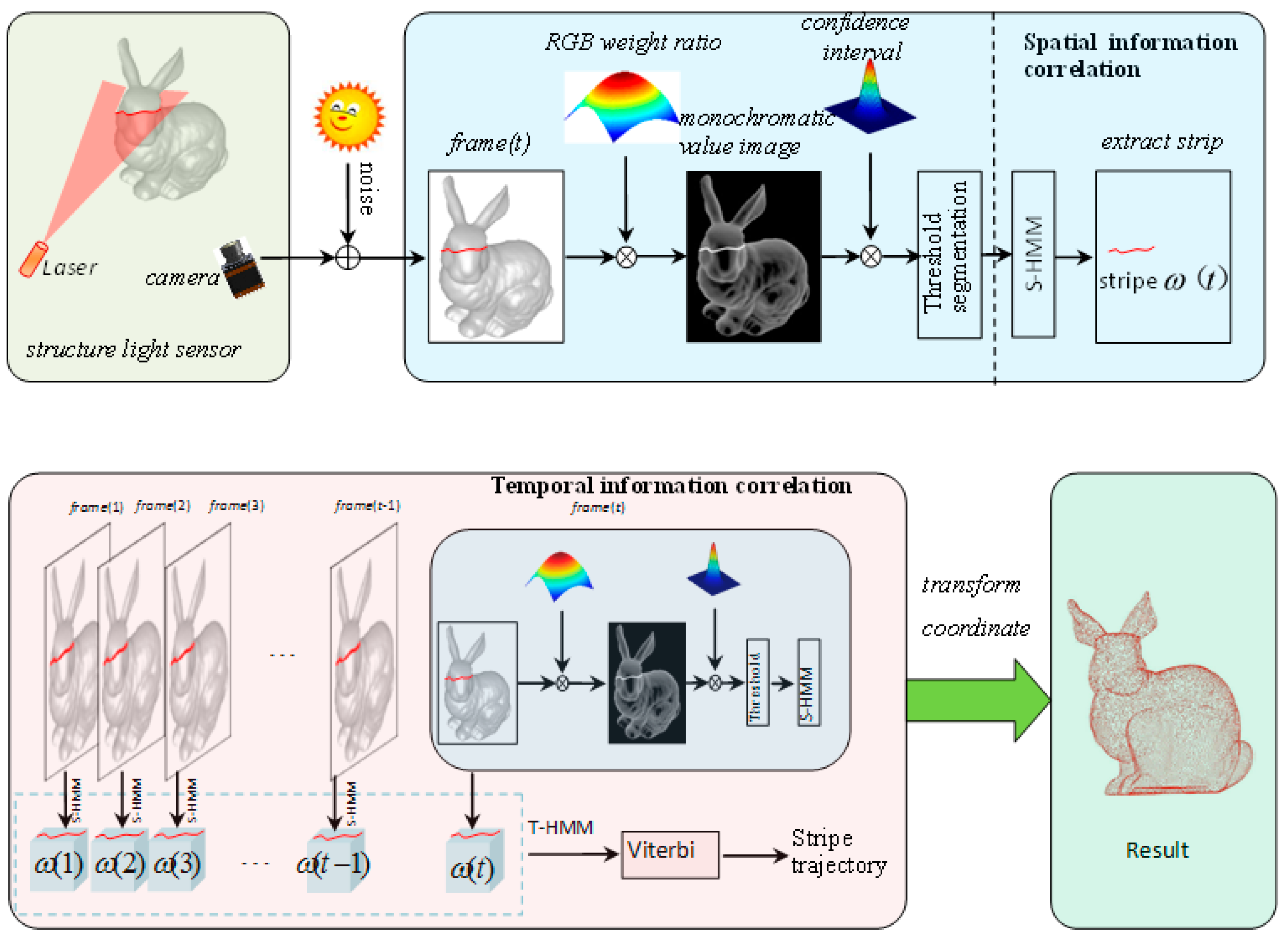
To solve the problem that a structured-light sensor is disturbed heavilyby environment noise in snow sculpture measurement, a 3D vision measurement method focused on light stripe extraction and tracking is proposed in this paper, as shown in Figure 2.
The original images mixed with noise collected by the structured-light sensor are classified based on RGB color space distribution and histogram image at first. Then optimal weight combination of RGB is constructed, and the color image is transformed into a monochromatic value image with high SNR. At last, a Decision Tree Model is established in a spatial and temporal context (STC-DTM) to extract and track the laser stripe. The result of the model after coordinate system transformation is a 3D measurement point cloud. This method improves the performance of a measurement system through image processing technique without changing the components of the structured-light sensor. It is universal for other similar 3D measurements.
The remainder of this paper is organized as follows. Section 2 provides details of the method and their algorithms. Section 3 describes the result of experiments for evaluating the accuracy, stability and speed of the method. The final section discusses and concludes the paper.

2. Methods

2.1. Noise Classification

The laser stripe in a structured-light image is the foreground, while othersignals interfering with the stripe extraction are noise. By analyzing snow sculpture measurement in actual scene, we found the main noise is from sunlight, shadows, surface color, surface reflections, and occasionally colored lights. As multiple types of noise are superimposed on images, it is hard to analyze such multi-source noise by constructing an optical path model.
In space distribution, light and surface color are global noise, whereas shadow, surface texture, and reflections are local. Snow sculpture is generally located in an open field, surrounded by snow. Since there are generally no colored buildings, flowers or other objects around, the possibilityof color pollution can be virtually eliminated.During measurement, the structured-light scanner is calibrated with sunlight. According to color distribution, sunlight and shadow usually have similar R, G, and B components, whereas the color values of colored light and surface colors are usually higher in one color dimension. Reflective noise is related to illumination and surface characteristics, and shows localized high intensity. The laser stripe isoverlaid by a large amount of environmental noise under sunlight, and the intensity distribution in R, G and B space is very close, thus presentinga single peak in the histogram, as shown in Figure 3. Conversely, the similarity between the three histograms is greatly reduced when there is interference from colored light or surface color. In the case of surface reflection, the similarity of intensity in space distribution decreases.
Based on the above analysis of color histogram, a qualitative description of the ambient noise in R, G and B space is made, which representsan approximate Gaussian distribution with different mean values and variances, and it will guide the color value space transformation.

2.2. Monochromatic Value Space Transformation

RGB color space sometimes does not show part of information we need, and some important information cannot be distinguished from the color space. Therefore, transforming a color value space to a monochromatic value space is more conducive to the extraction of laser stripe. In this paper, a linear transformation is used because it does not cause large jumps, singular value points, or discontinuities, and is faster than nonlinear transformation [15]. A gray image is the most typical monochromatic value image generated by linear transformation.
In a discrete color snow sculpture image fij (with a size of M × N), the tristimulus values of the pixels are Rij, Gij and Bij. The linear transformation is defined as Equation (1).
F i j = w r R i j + w g G i j + w b B i j
where Fij is the monochromatic value image after transformation, and i and j represent the row and column indexes of pixelsrespectively, with I = 1, 2 …, M, j = 1, 2 …, N, w r , w g , w b R . From Equation (1), the monochromatic value image is determined by the transformation coefficients. So, we need to define anobjective function to search for theoptimal w r , w g and w b to highlight the laser characteristics.
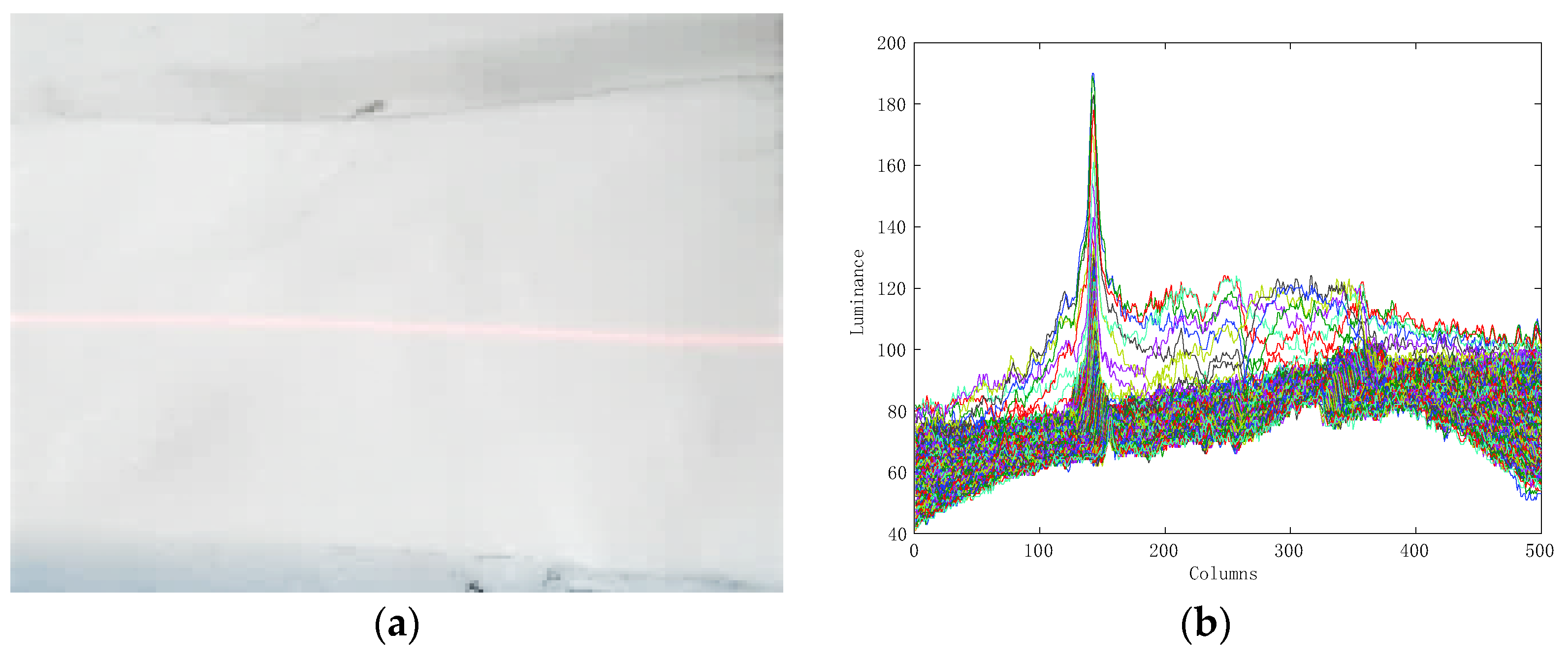
The projected stripe of the laser is relatively concentrated and presents a concise structure, and its profiles showing all the luminance row vectors are shown in Figure 4. There is a high contrast between the laser and background, implying a highSignal to Noise Ratio (SNR). The objective function should make full use of this characteristic so that the laser stripe can be extracted easily after transformation. Therefore, the objective function is taken as a measure of the contrast.
The pixel values in the laser stripe are close to their averages in Figure 4. In these areas, the contrast increases with energy concentration, and the waveform is steep, suggesting that kurtosis is high. This can be seen as a contrast between the laser stripe and the background. Thus, it is reasonable to choose the kurtosis to define the contrast. The kurtosis K is defined as Equation (2).
K = κ 4 κ 2 2 = μ 4 σ 4 3 ,
where κ 4 is the fourth cumulant, κ 2 is the second cumulant, and μ 4 and σ 4 are the mean of fourth moment and the square of the variance t of the probability distribution respectively. In particular, the kurtosis is zero in the case of normal distribution.
We expect that the laser stripe has the maximum kurtosis after transformation, while the noise signals from background have very low kurtosis, suggesting they are very disordered. In signal systems, disorder is synonymous with entropy. Entropy is affected by the amount of information and its random properties. The more information there is, the more disordered the signalsare, and the greater the entropy is. Wiggins [16] first used the minimum entropy deconvolution technique and called it the minimum entropy method. Therefore, maximizing kurtosis is equivalent to minimizing entropy, and the transformation model can be called the minimum entropy model. When K is less than 0 or if the signals come from a pulse source, minimizing is better than maximizing for the purpose of this study [17,18]. Therefore, the objective function can be further defined as Equation (3).
a b s ( K ) = | μ 4 σ 4 3 | ,
Equation (3) is fully differentiable, thus the maximizing function can be defined as Equation (4).
K 2 = ( μ 4 σ 4 3 ) 2 ,
The monochromatic value image F i j obtained after transformation is regarded as a multi-channel signal (with N segments and M elements per segment), and the Kurtosis can be written as
E = K 2 = ( j = 1 N i = 1 M ( F i j μ j ) 4 ( i = 1 M ( F i j μ j ) 2 ) 2 3 ) 2 ,
where μ j is the mean of column j in the image F i j .
The solution of maximizing (5) is given in Equation (6):
E w r = E w g = E w b = 0 ,
Obviously, it is difficult to solve the above equation. We can learn such knowledge from Robert t. Collins et al. [19]. The continuous coefficient w r , w g and w b in Equation (1) determine an infinite color feature set. To calculateexpediently, w r , w g and w b are discretized as integersconfined in [−2,2], and some common color spaces and models are also covered by this range, such as R + G + B, R–B, and so on, implying that it is feasible.
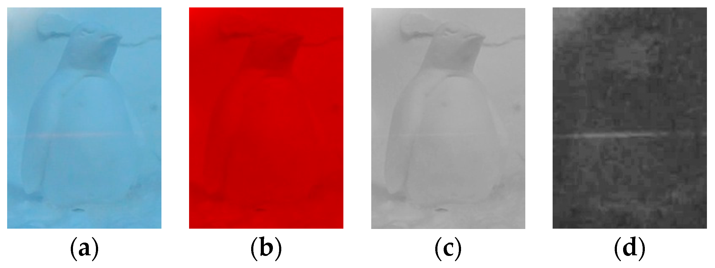
The laser used in the paper is red, and R component of the original image is higher in content than the other components, so limit w r 0 . The value ranges of w r , w g and w b are w r { 0 ,   1 ,   2 } , w g ,   w b { 2 ,   1 ,   0 ,   1 ,   2 } , where w r , w g and w b are not allowed to be zero at the same time. Then the coefficient vector can be solved by the traversal method. In Figure 5, a red single line laser is used. The optimal coefficient vector of the captured image is ( w r ,   w g ,   w b ) = ( 1 ,   1 ,   0 ) , and the monochromatic value space is R–G, whose transformation result of laser stripe is shown in Figure 5d. For comparison, Figure 5c shows the result in typical gray scale space ( w r ,   w g ,   w b ) = ( 0.30 ,   0.59 ,   0.11 ) . It is obvious that R–G space has more advantages in noise suppression and better SNR is obtained from it. The laser stripe is clearly distinguished from the background in R–G space, and the amount of data is only one third of the original image in Figure 5a.
To reduce harm of cold environment to people, we usually measure snow sculpture in the daytime. Also, snowy days are not chosen to avoid uneven distribution of new snow and its impact on measurement results. The R, G, B weights in the algorithm of this paper are dynamically changed. During each measurement, we readjust the parameters according to the calculation results to adapt to the measurement environment at that time.

2.3. Stripe Extraction and Tracking

After image preprocessing, global noise such as illumination is eliminated to the maximum, and the geometry edge of the laser stripe is kept continuous. However, some high light regions caused by strong reflection of snow sculpture surface are similar to laser projection, and the laser stripe presents different deformations along the texturedtarget surface, which can cause a large deviation during laser Stripe extraction and tracking. With traditional methods it is difficult to balance robustness, accuracy and real-time performance. In this paper, a Decision Tree Model based on spatial and temporal context (STC-DTM) is proposed to solve these problems.

2.3.1. Establishment of aSpatial Decision Tree Model(S-DTM)

In a single frame, there are two basic spatial constraints between thelaser stripe and background nearby: continuity and uniqueness [20]. Although thelaser stripe is a smooth and continuous line, the jump or break points indicate it is shaded. In addition, in the same frame, thelaser stripe cannot appear in more than one place (parallel or grid light stripe as a whole). Based on these constraints, the image pixels can be classified as two states: on or off thelaser stripe. Therefore, stripe extraction can be considered a dichotomy of decision trees, taking the pixels in each column of the image as a sample set, and thenbeing classified by selected features column by column.
The brightness distribution of a laser stripeis shown in Figure 6. We can learn from the figure thatthe central point is much brighter than neighboring points, and the distribution is continuous. So, the brightness of central points is very close between adjacent columns, and their distance is usually very small. Therefore, the brightness difference and the distance are candidate features for our study.
The laser stripe represents foreground information in the image, and it can be segmented effectively by the center of mass [14,21], which can be used to thin the light stripe. Canny edge detection is performed on the obtained monochromatic image to find edge pixel points, and match adjacent edge pixel points in each column to form point-pairs. In this way, the laser stripe presents a series of point-pairs. The distance between point-pairs is relatively small and their positions are concentrated. Moreover, the brightness in the point-pairs is also very similaron the corresponding monochromatic value image. So, we can calculate the center-of-mass position of R component for each point-pair by Equation (7).
M i ( w ) = j max i w 2 j max i + w 2 I i , j × j j max i w 2 j max i + w 2 I i , j , i [ 0 , n ) , j [ 0 , m ) ,
where w is window value (in the unit of pixel) of the calculated area, Iij is brightness value of the pixel at row i and column j on the image, and Mi(w) is column coordinates. After obtaining a series of brightness peaks, the laser stripe is refined into a chain of laser skeleton, as shown in Figure 7a. However, because of noise, there cannot be only one center-of-mass point in each column, and the light stripe skeleton must be accompanied by some noise points, so we must classify it further.
All the center-of-mass positions obtained in each column are taken as a position set of potentiallight stripe center points, and each position is represented as ωr(t), t = 1, 2 … T, where T is step(column) number of the image, r is the index at step t, and r ∈ [1, R(t)], R(t) is the amount of center-of-mass points at step t, as shown in Figure 7b.The coordinates of the edge pixel point on step t are [t, er(t)].The mean R component of all the pixels in the point-pair ([t, er(t)], [t, er+1(t)]) is mr(t), and thenthe brightness difference of the center-of-mass points between adjacent columnscan be described as Equation (8).
f i j = | m i ( t 1 ) m j ( t ) | ,
where i is the ith point at step (t−1), and j is the jth point at step t.
In addition, the distance between the centers of mass is also an important feature to judge whether they are the center points of the laser stripe, because the center points on the laser stripe do not change position suddenly. The Euclidean distance between two pixel points can be expressed as
d i j = ( c i ( t 1 ) c j ( t ) ) 2 + 1 ,
where c i ( t 1 ) and c j ( t ) are column coordinates of the two center-of-mass points.
The selected features are substantiated with data to derive Hf and Hd, which are the upper limit values of fij and dij respectively, with Gain(fij) > Gain(dij). So, the position set is classified by brightness difference fij at first, and then estimated by distance dij. The process of thelaser stripe extraction by S-DTM is shown in Figure 7b. The result in Figure 7c shows thelaser stripe is smoother and clearer, and noise has been well eliminated.

2.3.2. Establishment of aTemporal Decision Tree Model (T-DTM)

Similar to spatial context correlation, there is a strong temporal relationship between a light stripe and its background in video frame sequences. A traditional research about target tracking proposes that the local context of a current frame helps predict the location of light stripe in the next frame, because the shape, color, position of the target will not change muchbetween adjacent frames, and the rate of change is relatively stable [22,23]. Video sequences captured by a structured-light sensor also have the same characteristics. Ideally, laser linesin adjacent frames are represented as many line segments and arcs with similar shape, area and color, unlessthey are changed by the texture and reflection of snow sculpture surface, sensor movement and so on. Therefore, the line segments and arcs in each frame may or may not be on the laser stripe, and they also can be classified by a decision tree.
Several possible laser strip regions, which include the optimal solution and several suboptimal solutions of the S-DTM, are defined as a series of sub-windows Wn(k) = (x, y, I, Δ, s), where x and y are size of the window, I is mean brightness of thelaser stripe in the window, Δ is the change rate of tracking result relative to the previous frame, s is the scale factor, s ∈ [0.1, 10], n is the amount of candidate windows per frame, n ∈ [1, N(k)], N(k) is the amount of sub-windows at step k, k = 1, 2, …, F, and F is the number of the frame. Each sub-window Wn (k) is defined as a positionset of the current frame as shown in Figure 8, and measurable features between two adjacent frames are expressed as Equations (10) and (11).
P m n = ( x ¯ m ( k ) x ¯ n ( k 1 ) ) 2 + ( y ¯ m ( k ) y ¯ n ( k 1 ) ) 2 ,
I m n = | I m ( k ) I n ( k 1 ) | ,
where P m n and I m n present the position and brightness change between Wm(k) and Wn(k−1) respectively. In sub-window Wn(k), the average coordinates of all pixels on the laser stripe are ( x ¯ n ( k ) , y ¯ n ( k ) ) and the mean brightness of R component is In(k).
Considering the speed and direction of the scanning device, Equation (10) is rewritten as Equation (12).
P m n = ( x ¯ m ( k ) ( x ¯ n ( k 1 ) + 0 τ d u ) ) 2 + ( y ¯ m ( k ) ( y ¯ n ( k 1 ) + 0 τ d v ) ) 2 ,
where du and dv represent the velocity of the scanner in the u and v directions of the image space respectively, and τ is the interval between adjacent frames. So, the change rate of tracking position PΔ is described as Equation (13).
P Δ = P m n ( k ) P m n ( k 1 ) ,
The selected features are substantiated with data to derive HI and HΔ, which are the upper limit values of Imn and PΔ respectively, with Gain(PΔ) > Gain(Imn). The sub-window position set is then classified according to the gain values in proper order. The process of thelaser stripe tracking by T-DTM is shown in Figure 8, where the filled circles represent the laser stripe positions.
At this point, the STC-DTM has beenestablished. Here S-DTM and T-DTM are not in a cascade relation, but unified as a whole. The video collected by structured-light sensor is the input of STC-DTM, and the output is a series of smooth centerline tracks, which are also a global optimal solution of the model. Although the input of the temporal model depends on the output of the spatial model, optimal solution of the whole model depends on the original data set and the feature set. The optimal solution of the spatial model may be suboptimal in the temporal model, and vice versa.
According to the inherent calibration equation of the structured-light sensor, the tracksfrom STC-DTM are transformed from an image coordinate system to a sensor coordinate system, and then transformed to a global coordinate system [24] to finally obtain the point cloud data of the snow sculpture surface.

3. Results

To evaluate the validity and applicability of the method proposed in this paper, some experiments have been carried out. In the experiments, the algorithms are implemented in C++ and tested with an Intel Core i7-4790CPU of 3.6 GHz. In the structured-light device, a red single line laser projector of 650 nm and a color camera of SONY 1/4-in Charge coupled device(CCD) are used, and the angle between them is fixed at 45°. The video capture speed is 25 frames per second, and the image size is 640 × 480 pixels, 5.6 μm × 5.6 μm/pixel, with 8 mm of focal length, and the laser line width is about 2 mm.

3.1. Accuracy Test

In this section, a standard cube, a snow sculpture and a conventional object are measured, and then mean error and root mean square (RMS) error are calculated, respectively. The snow sculpture is large without a standard size, so the value measured by high-precision instrument is taken as the standard value, and the value measured by the method proposed in this paper is taken as the measurement value. The feature distance is used to evaluate measurement accuracy, to avoid the error caused by transformation of point coordinates. The standard value is d, and the measurement value is d′. Then the mean error can be expressed as Equation (14).
Δ d = 1 n i = 1 n ( d i d i ) ,
where n is the number of the selected feature line segments, with i = 1, 2, , n.

3.1.1. Standard Cube Measurement

In the experiment, a standard cube with black and white grid is designed. The size of the cube is 200 mm × 200 mm × 200 mm, the mesh of which is 20 mm × 20 mm, and the uncertainty is 0.01 mm. Six positions of the cube are chosen randomly, where 13 feature distances on the laser line are selected, as shown in Figure 9. The standard values are measured by the vernier caliper (0.02 mm), and the result is shown in Table 1, where (dx,dy,dz) and (d′x,d′y,d′z) represent the values in X, Y and Z directions of the standard value d and measurement value d′ respectively in global coordinates.
The RMS error of the feature distance is 0.125, and (0.049, 0.147, 0.113) in X, Y and Z directions. The mean error of the feature distance is 0.046 mm, and the maximum errors in X, Y and Z directions are 0.099 mm, 0.409 mm and 0.313 mm, respectively.

3.1.2. Snow Sculpture Measurement

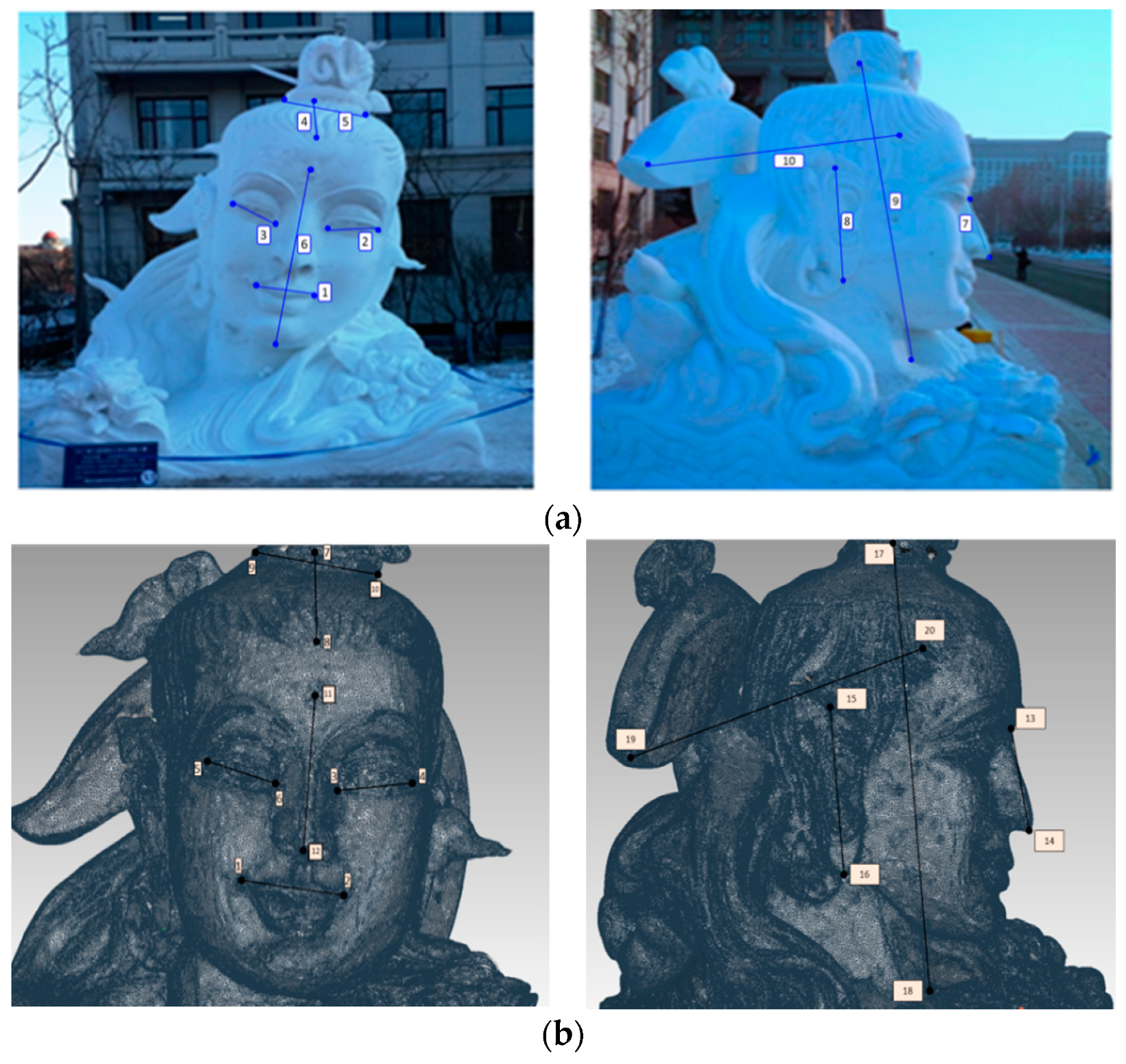
A snow sculpture is selected with the approximate size of 3000 mm × 3000 mm × 3000 mm. Twenty feature points are selected on the surface of the snow sculpture, and 20 blue round marking patches with a diameter of about 2 mm and a thickness of 0.1 mm are attached to these points, as shown in Figure 10. At first, a laser tracker is used to measure each pair of feature points for three times, and an average is derived. The distance between two points is then calculated as the standard value. Next, the center of corresponding blue marking patches are in the point cloud generated by the structured-light device. The distance between them is obtained. The average of three measurements is taken as the final measurement. The resultsare shown in Table 2.
The RMS error of the feature distance is 0.722, and (0.755, 0.588, 0.862) in X, Y and Z directions. The mean error of the feature distance is 0.574 mm, and the maximum errors in X, Y and Z directions are 1.522 mm, 1.033 mm and 1.409 mm, respectively.

3.1.3. Conventional Object Measurement

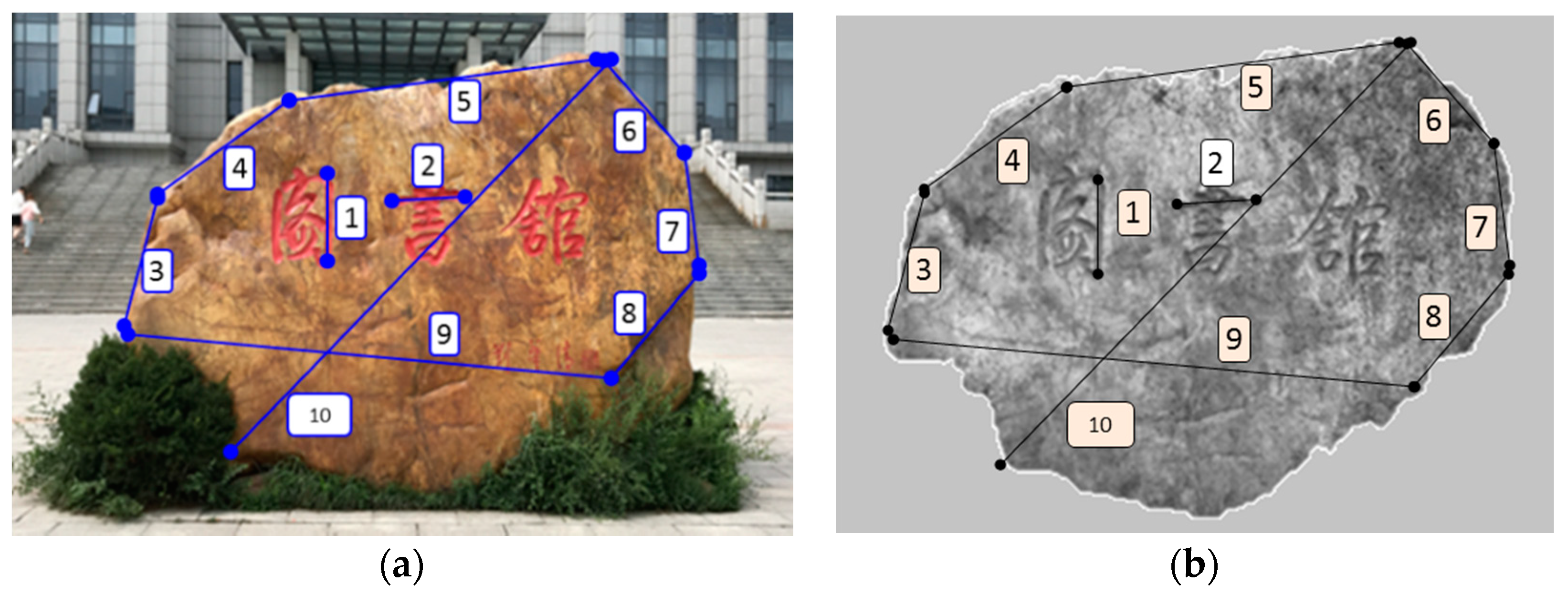
In the above two experiments, the measurement accuracy is quite different, so the third object is tested. The third measured object, as a conventional object, is irregular, opaque and less reflective, with a size of 4000 mm × 1000 mm × 2000 mm. 10 feature distances are selected as shown in Figure 11. The measurementsareprocessedin the same way as that in Section 3.1.2, and the result is shown in Table 3.
The RMS error of the feature distance is 0.508, and (0.539, 0.297, 0.435) in X, Y and Z directions. The mean error of the feature distance is 0.159 mm, and the maximum errors in X, Y and Z directions are 0.782 mm, 0.402 mm and 0.625 mm, respectively.

3.2. Speed and Robustness Evaluation

In the present study, two snow sculpture scenarios are selected, corresponding to the lighting conditions at 7:00 a.m. (with little sunlight) and 10:00 a.m. (with much sunlight) respectively. By using structure from motion method with patch-based multi-view stereopsismethod processing(PMVS-SFM) brought forward by Furukawa et al. [25], laser scanning method using Leica RTC360 and the method proposed in this paper, 3D reconstruction is performed, with the results given in Figure 12 and Figure 13, respectively.
It can be seen from the test results that for snow sculpture with complicated surface texture, a dense 3D point cloud generated with PMVS-SFM image reconstruction method of Furukawa contains more invalid areas, preventing it from well reproducing the original appearance of the snow sculpture. The measurement grows even poorer with the increase of exposure to sunlight. Laser scanning method is less sensitive to sunlight, but provides a relatively sparse point cloud with vague details. Moreover, its laser measurement accuracy of surface texture of the snow sculpture is affected by secondary reflection characteristics of the surface. By comparison, the method proposed in this paper successfully addresses the impact of sunlight and secondary reflection of snow, thus leading to more satisfactory imaging. The benefits include clearer texture and higher stability and accuracy.
Meanwhile, the average execution time of 1000 frames is calculated to be 21.3 ms. It is enough to ensure real-time nature of the normal video capture operation at a speed of 25 frame/s.

4. Discussion

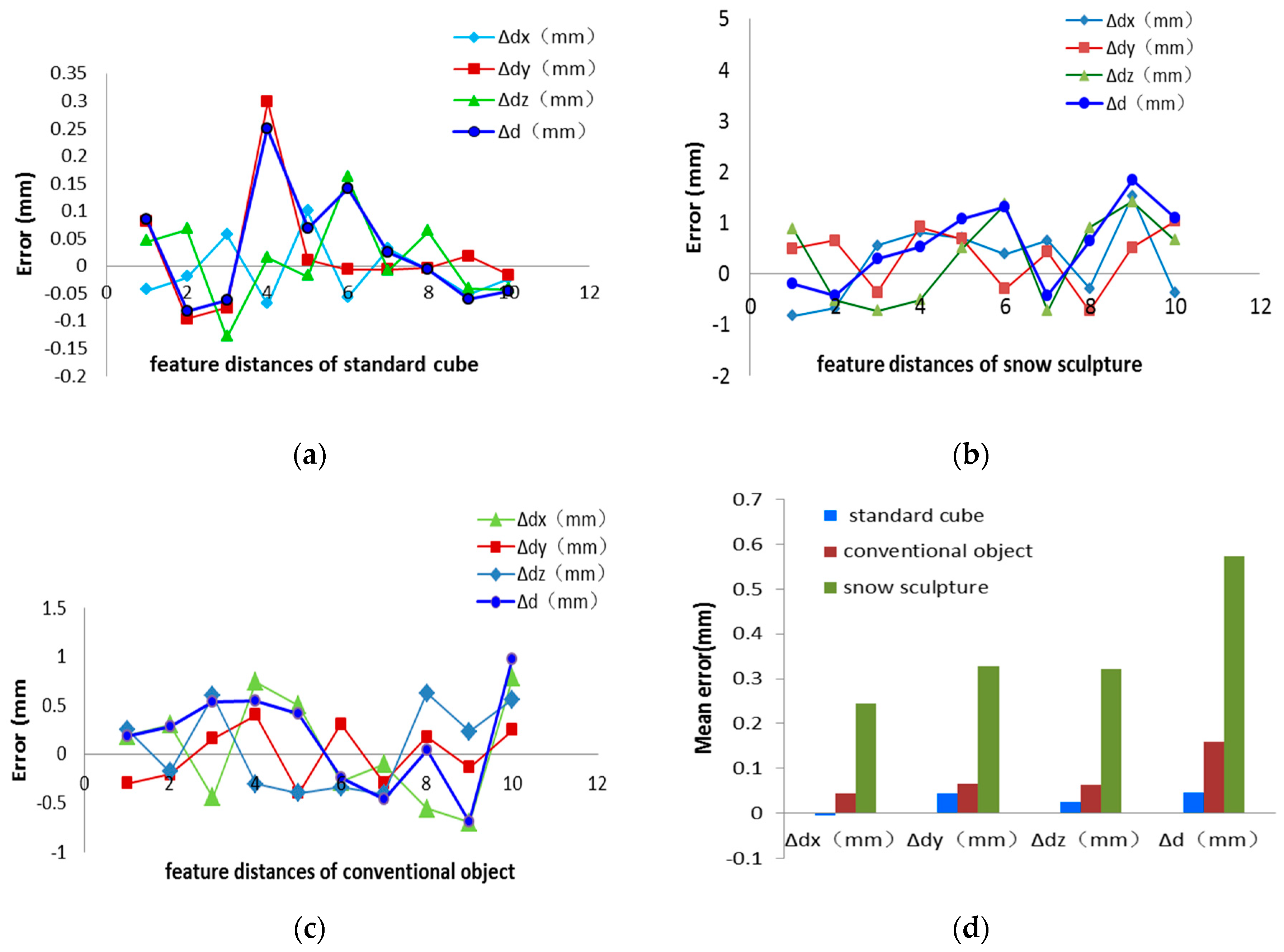
The measurement error statisticalresult of the three tests in Section 3.1 are shown in Figure 14. The errors are all distributed in a certain range, and the overall measurement accuracy of snow sculpture is lower than that of the other two measurement objects, with large local errors. The reason is analyzed as follows.

4.1. Light Environment and Optical Characteristics of the Measured Object Surfaces Affect the Measurement Accuracy

The surface characteristics of the measured objects include color, texture, brightness, roughness, etc., which produce different noise signals on the collected images. In the outdoor environment, the snow sculpture has strong reflection, complex texture, shadow and other factors that affect the measurement accuracy, which are different from the surface characteristics of standard cube and conventional object, leading to reduced accuracy. It is shown in Table 4 that the multiple additional noise sources lead to the decrease of accuracy and speed, but the measurement error is acceptable for large snow sculpture. It is also provedthrough the tests that the method is applicable in outdoor complex light environment, meaning that it can provide technical support for digital archiving of snow sculptures.

4.2. Large Local Error Is Related to Complex Texture and the Length of the Feature Distance

Some large local errors appear at feature distances where the texture is complex, such as No.9 on snow sculpture, No.10 on conventional object, because serious distortion and occlusion of laser stripe are caused by concave–convex surfaces and lead to inaccurate stripe extraction. In addition, some long feature distances have large errors, because the accumulated errors increase during the measurement without mark points. Therefore, high-accuracy splicing method without mark points is a main task in the next-stage research to improve the accuracy.

5. Conclusions

This paper proposes an accurate, fast and robust 3D measurement method based on structured-light used in complexity light environment. First, an optimal monochromatic value space based on a minimum entropy model is selected for segmentation to maximize the elimination of global noise. Then, a Spatial and Temporal Context Decision Tree Model (STC-DTM) is constructed toextract and track the laser stripe accurately to obtain an accurate and dense 3D point cloud. Finally, the experiments show that this method is effective and applicable to CCD cameras without optical filtering function. Moreover, the method is universal for 3D field measurement and reconstruction in the sectors of industrial detection, cultural archaeology and criminal investigation, and therefore has a good application prospect.

Author Contributions

Conceived the method and edited themanuscript, W.L.; investigation and wrote the paper X.Z.; conceived the method and designed the experiments W.L. and L.H.; project administrationand performed the experiments, L.Z. and W.L. All authors have read and agreed to the published version of the manuscript.

Funding

This research was funded by National Science Foundation of China (61501132), National Natural Science Foundation of Heilongjiang Province (LH2020E012) and the China Postdoctoral Science Foundation (2016M601399).

Acknowledgments

The authors would like to thank the associate editor and the reviewers for their helpful comments, which improved the quality of this paper.

Conflicts of Interest

The authors declare no conflict of interest.

References

  1. Dewar, K.; Meyer, D.; Li, W.M. Lanterns of ice, sculptures of snow. Tour. Manag. 2001, 22, 523–532. [Google Scholar] [CrossRef]
  2. Huang, Z.; Zhang, L. Analysis of and Research into Foreign Factors That Drive China’s Ice-Snow Tourism. In Communications in Computer and Information Science, Proceedings of the Advances in Applied Economics, Business and Development, Dalian, China, 6–7 August 2011; Springer: Berlin/Heidelberg, Germany, 2011; pp. 422–427. [Google Scholar]
  3. Li, Y.; Chen, Z.Y.; Wang, C.M. Research on the innovation and development of Harbin ice and snow tourism industry under the background of Beijing winter Olympic Games. China Winter Sports 2018, 2, 15. [Google Scholar]
  4. Di, H.N. On the digital technology in the protection of ancient buildings. Cult. Relics Apprais. Apprec. 2018, 3, 130–132. [Google Scholar]
  5. Koeva, M.; Luleva, M.; Maldjanski, P. Integrating Spherical Panoramas and Maps for Visualization of Cultural Heritage Objects Using Virtual Reality Technology. Sensors 2017, 17, 829. [Google Scholar] [CrossRef] [PubMed] [Green Version]
  6. Kuznetsova, I.; Kuznetsova, D.; Rakova, X. The use of surface laser scanning for creationof a three-dimensional digital model of monument. Procedia Eng. 2015, 100, 1625–1633. [Google Scholar] [CrossRef] [Green Version]
  7. Han, L.F.; Hou, Y.D.; Wang, Y.J.; Liu, X.B.; Han, J.; Xie, R.H.; Mu, H.W.; Fu, C.F. Measurement of velocity of sand-containing Oil-Water two-phase flow with super high water hold up in horizontal small pipe based on thermal tracers. Flow Meas. Instrum. 2019, 69, 101622. [Google Scholar] [CrossRef]
  8. Gupta, M.; Yin, Q.; Nayar, S.K.; Iso, D. Structured Light in Sunlight. In Proceedings of the IEEE International Conference on Computer Vision, Sydney, Australia, 3 March 2014; pp. 545–552. [Google Scholar]
  9. Gelabert, P. Comparison of fixed-pattern and multiple-pattern structured light imaging systems. Proc. Spie Int. Soc. Opt. Eng. 2014, 8979, 342–348. [Google Scholar]
  10. Kinect Outdoors. Available online: www.youtube.com/watch?v=rI6CU9aRDIo (accessed on 2 December 2015).
  11. O’Toole, M.; Mather, J.; Kutulakos, K.N. 3D Shape and Indirect Appearance by Structured Light Transport. In Proceedings of the IEEE Conference on Computer Vision and Pattern Recognition (CVPR), Columbus, OH, USA, 23–28 June 2014. [Google Scholar]
  12. Steger, C. An unbiased detector of curvilinear structures. IEEE Trans. Pattern Anal. Mach. Intell. 1998, 20, 113–125. [Google Scholar] [CrossRef] [Green Version]
  13. Usamentiaga, R.; Molleda, J.; García, D.F. Fast and robust laser stripe extraction for 3D reconstruction in industrial environments. Mach. Vis. Appl. 2012, 23, 179–196. [Google Scholar] [CrossRef]
  14. Haverinen, J.; Röning, J. An Obstacle Detection System Using a Light Stripe Identification Based Method. In Proceedings of the IEEE International Joint Symposia on Intelligence and Systems, Rockville, MD, USA, 23 May 1998; pp. 232–236. [Google Scholar]
  15. Zhang, L.G.; Sun, J.; Yin, G. Across Structured Light Sensor and Stripe Segmentation Method for Visual Tracking of a WallClimbing Robot. Sensors 2015, 15, 13725–13751. [Google Scholar] [CrossRef] [PubMed] [Green Version]
  16. Wiggins, R.A. Minimum entropy deconvolution. Geoexplorafion 1978, 16, 21–35. [Google Scholar] [CrossRef]
  17. Mcdonald, G.L.; Zhao, Q.; Zuo, M.J. Maximum correlated kurtosis deconvolution and application on gear tooth chip fault detection. Mech. Syst. Signal Process. 2012, 33, 237–255. [Google Scholar] [CrossRef]
  18. Mathis, H.; Douglas, S.C. Bussgang blind deconvolution for impulsive signals. IEEE Trans. Signal Process. 2003, 51, 1905–1915. [Google Scholar] [CrossRef]
  19. Collins, R.T.; Liu, Y.; Leordeanu, M. On-line selection of discriminative tracking features. IEEE Trans. Pattern Anal. Mach. Intell. 2005, 27, 1631–1643. [Google Scholar] [CrossRef] [PubMed]
  20. Kai, Q.; Xiuhong, C.; Baiwei, S. Robust fast tracking via spatio-temporal context learning. Comput. Eng. Appl. 2016, 52, 163–167. [Google Scholar]
  21. Yuehua, L.; Jingbo, Z.; Fengshan, H.; Lijian, L. Sub-pixel extraction of laser stripe center using an improved gray-gravity method. Sensors 2017, 17, 814. [Google Scholar]
  22. Sun, J.H.; Wang, H.; Liu, Z.; Zhang, G.J. Fast extraction of laser strip center in dynamic measurement of rail abrasion. Opt. Precis. Eng. 2011, 19, 690–695. [Google Scholar]
  23. Li, Y.; Li, Y.F.; Wang, Q.L.; Xu, D.; Tan, M. Measurement and defect detection of the weld bead based on online vision inspection. IEEE Trans. Instrum. Meas. 2010, 59, 1841–1849. [Google Scholar]
  24. Zhang, L.; Ke, W.; Ye, Q.; Jiao, J. Anovel laser vision sensor for weld line detection on wall-climbing robot. Opt. Laser Technol. 2014, 60, 69–79. [Google Scholar] [CrossRef]
  25. Furukawa, Y.; Ponce, J. Accurate, Dense, and Robust Multiview Stereopsis. IEEE Trans. Pattern Anal. Mach. Intell. 2010, 32, 1362–1376. [Google Scholar] [CrossRef] [PubMed]
Figure 1. Snow sculpture artwork.
Applsci 11 03324 g001
Figure 2. The process of 3D vision measurement based on structured light.
Applsci 11 03324 g002
Figure 3. (a) A snow sculpture (penguin) image scanned by structure light in sunlight; (bd) Color histograms of (a) in R, G and B space.
Applsci 11 03324 g003
Figure 4. Profiles of the laser. (a) Images captured including laser stripe on snow sculpture surface; (b) Luminance values row by row.
Applsci 11 03324 g004
Figure 5. The result of color feature transformation. (a) Original image; (b) R component image; (c) Grayscale image; (d) Monochromatic value of R–G image.
Applsci 11 03324 g005
Figure 6. Brightness distribution of a laser line.
Applsci 11 03324 g006
Figure 7. The process of the stripe extractionbyS-DTM, with“□” beingthe edge pixel point [t, er(t)] and“” thecenter-of-mass point ωr(t). (a) Thinning result by center-of-mass method; (b) Explanation of classification of S-DTMby takingthree columns of pixels from the red line in (a); (c) The resultof stripe extraction by S-DTM.
Applsci 11 03324 g007
Figure 8. The process of the stripe tracking by T-DTM. (a) Explanation of classification of T-DTM bytaking two frames; (b) The sketches of laser stripe tracking.
Applsci 11 03324 g008
Figure 9. Standard cube measurement; (a) 13 feature distances selected on the standard cube; (b) 13 feature distances on the 3D point cloud.
Applsci 11 03324 g009
Figure 10. Snow sculpture measurement; (a) 10 feature distances selected on the snow sculpture; (b) 10 feature distances on the 3D point cloud.
Applsci 11 03324 g010
Figure 11. Conventional object measurement; (a) 10 feature distances selected on the conventional object; (b) 10 feature distances on the 3D point cloud.
Applsci 11 03324 g011
Figure 12. Three-dimensional reconstruction of snow sculptures at 7:00 a.m. (a) Snow sculpture front; (b) 3D reconstruction results using PMVS-SFM; (c) 3D reconstruction results using laser scanning method;(d) 3D reconstruction resultsusing our method.
Applsci 11 03324 g012
Figure 13. Three-dimensional reconstruction of snow sculptures at 10:00 a.m. (a) Snow sculptures side; (b) 3D reconstruction results using PMVS-SFM; (c) 3D reconstruction results using laser scanning method; (d) 3D reconstruction resultsusing our method.
Applsci 11 03324 g013
Figure 14. The measurement errors and their components in x, y and z directions. (a) Error distribution of standard cube measurement; (b) Error distributionof snow sculpture measurement; (c) Error distributionof conventional object measurement; (d) Mean error comparison of three measurements.
Applsci 11 03324 g014
Table 1. The result of standard cube measurement.
Standard ValueMeasurement ValueError
dx
(mm)
dy
(mm)
dz
(mm)
d
(mm)
d′x
(mm)
d′y
(mm)
d′z
(mm)
d′
(mm)
Δdx
(mm)
Δdy
(mm)
Δdz
(mm)
Δd
(mm)
10.05752.39862.41981.4970.01352.47962.46481.583−0.0440.0810.0450.086
266.20066.2760.26493.67566.18066.1800.33193.593−0.020−0.0960.067−0.082
351.1451.95658.66577.85451.2021.88058.53677.7920.057−0.076−0.129−0.062
40.273118.47785.960146.3760.204118.57685.975146.627−0.0690.2990.0150.251
5119.6012.10087.924148.457119.7002.11187.905148.5260.0990.011−0.0190.069
60.28957.164119.454132.4280.23157.158119.615132.570−0.058−0.0060.1610.142
7116.33460.6230.097131.182116.36560.6170.088131.2070.031−0.006−0.0090.025
844.990118.1570.348126.43344.984118.1540.411126.428−0.006−0.0030.063−0.005
962.8772.721120.578136.01562.8252.740120.537135.955−0.0520.019−0.041−0.060
100.20069.578123.365141.6340.17769.562123.323141.589−0.023−0.016−0.042−0.045
11122.3117.5980.544122.548122.2847.5500.503122.518−0.027−0.048−0.041−0.030
120.005117.5430.199117.5430.030117.5280.135117.5280.025−0.015−0.064−0.015
130.0251.913116.542116.5580.0402.322116.855116.8780.0150.4090.3130.320
Mean error (mm)−0.0060.0430.0250.046
RMS errors (mm)0.0490.1470.1130.125
Table 2. The result of snow sculpture measurement.
Standard ValueMeasurement ValueError
dx
(mm)
dy
(mm)
dz
(mm)
d
(mm)
d′x
(mm)
d′y
(mm)
d′z
(mm)
d′
(mm)
Δdx
(mm)
Δdy
(mm)
Δdz
(mm)
Δd
(mm)
1394.526285.011105.542498.017393.696285.502106.424497.829−0.8300.4910.882−0.188
2402.012153.21422.123430.787401.328153.85821.599430.352−0.6840.644−0.524−0.435
3408.995179.56234.856448.034409.543179.19034.130448.3300.548−0.372−0.7260.296
4333.785389.215486.671706.930334.598390.123486.156707.4600.8130.908−0.5150.530
5494.594390.996190.462658.617495.294391.669190.962659.6870.7000.6730.5001.070
6265.123314.0141405.1021463.969265.510313.7171406.4611465.2800.387−0.2971.3591.311
7164.92097.126534.857568.070165.57297.549534.124567.6430.6520.423−0.733−0.427
8158.152299.1021135.2161184.563157.859298.3761136.1211185.208−0.293−0.7260.9050.645
9852.156256.9832668.2472812.784853.678257.4922669.6562814.6281.5220.5091.4091.844
10225.5621899.215389.5291951.827225.1871900.248390.1911952.921−0.3751.0330.6621.094
Mean error (mm)0.2440.3290.3220.574
RMS errors (mm)0.7550.5880.8620.722
Table 3. The result of conventional object measurement.
Standard ValueMeasurement ValueError
dx
(mm)
dy
(mm)
dz
(mm)
d
(mm)
d′x
(mm)
d′y
(mm)
d′z
(mm)
d′
(mm)
Δdx
(mm)
Δdy
(mm)
Δdz
(mm)
Δd
(mm)
12.02617.512431.588431.9482.21516.812431.788432.1370.1890.4020.2540.189
2411.31425.52722.123412.699411.61625.32121.945412.9780.302−0.206−0.1780.302
3112.56481.495710.525723.987112.12281.652711.121724.522−0.4420.1570.596−0.442
4919.468138.619511.2031061.115920.210139.021510.8991061.6640.7420.402−0.3040.742
52412.852215.665262.4212436.6432413.352215.268262.0212437.0600.500−0.397−0.4000.500
6365.133301.214416.230630.317364.847301.521415.889630.073−0.2860.307−0.341−0.286
7165.249118.259687.255716.667165.145117.966686.845716.202−0.104−0.293−0.410−0.104
8765.210412.036642.5311080.817764.652412.214643.1561080.862−0.5580.1780.625−0.558
93215.365168.249215.2233226.9493214.665168.112215.4563226.260−0.700−0.1370.233−0.700
103016.230215.2662101.5623682.4653017.012215.5142102.1223683.4390.7820.2480.5600.782
Mean error (mm)0.0430.0660.0640.159
RMS errors (mm)0.5390.2970.4350.508
Table 4. The relation between the noise and the results in the experiments.
IndexReflectionShadowSurface Color/
Color Light
Mean Error
(mm)
Speed
(ms/Frame)
Measured
Object
Standard cube(wood)weaknoneweak0.04618.9
Conventional object(stone)middlestrongstrong0.15920.7
Snow sculpture(snow)very
strong
very strongstrong0.57421.3
Publisher’s Note: MDPI stays neutral with regard to jurisdictional claims in published maps and institutional affiliations.