Abstract
Nowadays, there is a growing trend to incorporate renewables in electrical power systems and, in particular, wind energy, which has become an important primary source in the electricity mix of many countries, where wind farms have been proliferating in recent years. This circumstance makes it particularly interesting to understand wind behavior because generated power depends on it. In this paper, a method is proposed to synthetically generate sequences of wind speed values satisfying two important constraints. The first consists of fitting the given statistical distributions, as the generally accepted fact is assumed that the measured wind speed in a location follows a certain distribution. The second consists of imposing spatial and temporal correlations among the simulated wind speed sequences. The method was successfully checked under different scenarios, depending on variables, such as the number of locations, the duration of the data collection period or the size of the simulated series, and the results were of high accuracy.
1. Introduction
The electricity needs in daily life are assorted, and there are countless actions that consumers carry out daily, such as turning on lights, charging electronic devices or cooking [1]. Moreover, electricity production across the world has a growing perspective due to several causes, among which the new trend to use electric vehicles can be mentioned [2].
The negative impact of fossil fuel gas emissions on human health and also on the planet health raises the awareness about the harmful effects of such emissions [3], and due to this, different countries have agreed to limit global warming to a value lower than 2 °C concerning preindustrial era [4]. To ensure the compliance of greenhouse gas emissions reduction into the atmosphere, the European Union has published a guide showing different scenarios [5]. All of them involve an increasing trend in the use of renewables, as all hypotheses show that most of the energy supply in 2050 will be generated using renewables, and the energy transition from fossil fuels to them constitutes a problem of world concern [6]. Specifically, wind energy prevails both in the current market and in the future production trends, foreseeing a doubling of installed capacity in the next ten years in the most conservative case [7], mainly due to the low cost of wind energy produced in large wind farms. This cost can be lower than 0.05 $/kWh in the locations with the highest mean wind speed values [8].
Renewables depend on the variability of weather conditions. In the case of wind energy, the behavior of the primary resource, i.e., the wind, can be considered stochastic. However, in a given location, a set of measured wind speeds along a certain period can be described using some probability distribution [9], and the Weibull distribution is one of the most recommended and used for such a purpose [10,11,12].
The characterization of wind speed is achieved by measurements, and there are factors that can make it difficult to proceed, such as the presence of adverse weather conditions, meter errors, lack of measurements due to maintenance periods or communication problems. In addition, it can happen that the accuracy of the measurement devices is not as good as expected, and this can result in an alteration of the values of the collected data [13,14]. Additionally, in general, the wind speeds are measured at a given height that does not necessarily coincide with those of the wind turbine hubs [15,16,17]. These problems must be solved with the aim of accuracy since it is a critical factor when planning power generation [18,19]. By studying wind speed simultaneity in different locations, it is possible to obtain the wind energy production at each period in an easier way using traditional methods [20,21,22]. Thus, from the dependence on the wind speeds between nearby places, the problem can be reduced to calculate the probability in each scenario [23].
Analyzing the spatial correlations, the relationships between the wind speeds in different locations can be established. In this way, gaps that arise due to errors in the meter or in data capture can be covered, i.e., periods in which the data are not available, obtaining an accurate wind speed value in each moment and, in turn, of the power injected into the electrical network [24,25]. If temporal correlations are also calculated, it is possible to characterize the resource in a later gap, being able to anticipate possible errors and assuring a reliable wind speed value [26,27,28].
2. Methodology
The randomness of the wind speed, along with the possible failures in the data collection stage, does not allow users to get the power production easily and makes the calculation method a complex problem. The study of the simultaneity of a generation when there is wind energy injection in the system reveals a stochastic process, which includes uncertainty at each of the locations, and converts it into a deterministic one by assigning a value of probability to each place and making it possible to obtain a solution to the problem [23]. The degree of accuracy of the proposed algorithm increases when spatial and temporal correlations are considered. Taking this into account, in this paper, both kinds of correlations are considered. In the case of temporal correlation, a value of lag 1 is used.
As is detailed later, the process starts by considering that the random behavior of the wind speed at every location can be cumulatively described by a Weibull probability distribution function, an assumption generally accepted in wind energy studies. This enables the simulation of the wind speed randomness as a stochastic process with known probabilities. The Monte Carlo method is used with this aim [10].
Two major stages are developed. The first one consists of modeling, and in this stage, the correlations between the wind speeds of the different locations are obtained. The second one consists of simulating, and here the randomness of the wind speed sequences that can be generated in a certain period is reproduced, and in this stage, it is possible to cover the errors produced during the collection. As can be seen in Figure 1, each stage has its own steps, developed progressively until the objectives are achieved.
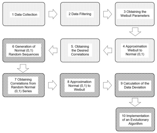
Figure 1.
Steps in developing the problem, where steps from 1 to 5 correspond to the modeling stage and steps from 6 to 10, to the simulation stage.
2.1. Modeling
The degree of simultaneity of the wind speeds at the different locations is obtained when carrying out the modeling stage. This phase is divided into the five steps exposed in the following sections.
2.1.1. Data Collection
A good performance of the model requires well-characterized wind speed data. In addition, it is required that the data collection periods for the evaluation of the wind simultaneity have identical features; this is to say, the starting and finishing times of data collection must coincide for the studied sequences of different locations, and with a minimum period of one year [29]. The previous sentence refers to 10 min mean wind speed values simultaneously measured at such locations.
The data needed to characterize the wind at a given place can have different origins, such as those obtained during a measurement campaign, those coming from wind farm anemometers or those collected in meteorological stations.
The fact must be mentioned that wind speed might have been measured at a height that can be different from the one of the wind turbine hubs. For example, in the case of meteorological stations, wind speeds are measured at a few meters above the terrain, i.e., 2, 5 or 10 m. The value of the wind speed at a different height can be calculated with the help of the knowledge of the ground roughness, characterized by the friction factor, and taking the shear effect into account [15].
2.1.2. Data Filtering
There are numerous possibilities of failures during the data collection period. There may be errors due to the meter, communication problems, adverse weather conditions, and others. In all these cases, it is impossible to characterize wind speed at the study points and, as a consequence, to accurately calculate the power that can be generated at each moment.
To perform the filtering process, it is only necessary to discard invalid and suspicious values, and it is important to avoid removing spaces produced by wrong values so that the chronology of the collected sequences keeps unmodified. Therefore, the value 0 is imposed in all these cases [30].
If the data collection height is not the same as that of the study, it is necessary to get the true value of the wind speed [15], and this is achieved by using Equation (1):
where is the wind speed at the study height, is the wind speed of the collected data, is the height of the wind turbine hub, is the height at which data were collected, and is the friction coefficient of the terrain.
On the other hand, to avoid troubles and facilitate calculations, conversion factors are performed to obtain all the units in the international system.
2.1.3. Obtaining the Weibull Parameters
After the filtering process, using Equation (2) involves the consideration that wind speed follows a Weibull distribution in all the locations, widely used in wind energy studies [10]. This equation describes the probability distribution function of such a distribution:
where is the wind speed, is the scale parameter, and is the shape parameter.
Both parameters are obtained by using the method of maximum-likelihood estimation, i.e., the scale parameter is estimated according to Equation (3), and the shape parameter according to Equation (4):
where , , is the length of the series, is the i-th wind speed value.
2.1.4. Approximation Weibull to Normal (0,1)
Values belonging to sequences that fit a Weibull distribution can be converted into values of sequences that follow a standardized Normal one, i.e., a Normal distribution with mean 0 and standard deviation 1, denoted as Normal (0,1). This is the next step, and the reason for pursuing it is that, as is explained in Section 2.2.2, the use of Normal (0,1) distributions makes it possible the induction of given correlations to the random sequences generated directly and keeping all the features of the distributions [18]. In other words, in statistics, it is a well-known fact that it is possible to get every number of normally distributed sequences satisfying a given correlation matrix. Normal (0,1) data can be obtained from Weibull ones by matching both cumulative distribution functions (CDF), as can be seen in Equation (5), where Weibull parameters obtained for each place must be dealt with:
where is the wind speed belonging to a Normal (0,1) distributed sequence, is the wind speed belonging to a Weibull distributed one, and is the inverse of the error function, where the error function is given by Equation (6):
is the time, and is a symbolic number.
Both directions of this conversion, from Weibull to Normal (0,1) and from Normal (0,1) to Weibull, are shown in Figure 2.
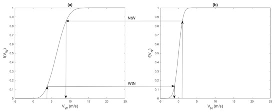
Figure 2.
Transformation between Normal (0,1) and Weibull distributions, where WtN shows the Weibull to Normal (0,1) direction and NtW the Normal (0,1) to Weibull direction: (a) Weibull cumulative distribution functions (CDF), (b) Normal CDF.
2.1.5. Obtaining the Desired Correlations
To finish the modeling stage, the relations between locations are achieved. For this, the correlations are calculated from the Normal standard distributed series of values obtained in the previous step. As was mentioned in Section 2.1.2, the positions of the values of the series are kept guaranteeing the correspondence in the calculation of the correlations, changing wrong values to zero. Thus, the correlations are calculated between pairs of locations, discarding the null values.
The correlations vary in the interval [−1,1], where +1 is equal to a perfect direct correlation, i.e., the variables move in the same direction; −1, corresponds to a perfect inverse correlation, i.e., the variables move in the opposite direction; and 0, to the nonexistence of correlation between the variables. Figure 3 shows these three correlation possibilities graphically [31].
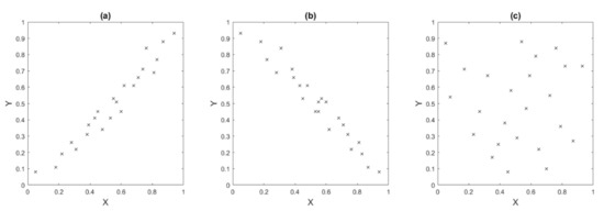
Figure 3.
Possibilities for normalized correlations: (a) positive correlation, (b) negative correlation, (c) no correlation.
The following paragraphs explain the types of correlations considered in this paper, i.e., spatial correlation, autocorrelation and cross-correlation.
- (a)
- Spatial correlation
Pearson’s correlation, , measures the force and the direction of the linear correlation of two variables and . This can be written as in Equation (7) with the quotient between covariance, , and the standard deviations, , , of the involved variables [31]:
As shown in Equation (8), the covariance provides information on how both variables evolve:
where is the value of sequence at time , is the mean value of , is the value of sequence at time and is the mean value of the . If , the trend of one of the variables to increase coincides with the trend of the other variable to decrease. If , both variables tend to increase or decrease simultaneously, or at least there is a certain similarity in both trends. If , there is not a common trend [31].
The standard deviation of the considered variables, Equations (9) and (10), provides the dispersion of the data around the mean value. The greater the standard deviation is, the greater dispersion and vice versa [31]:
As can be seen in Equation (11), the values obtained for every two variables take part in a correlation matrix of size , where is the total number of locations.
Due to the use of the Pearson’s correlation coefficient, the correlation matrix has some particularities:
- Elements of the main diagonal equal 1, Equation (12)
- It is symmetrical, Equation (13)
- It is positive semidefinite.
It can be said that the number of calculations depends on the number of correlation values between different locations. Therefore, it is only necessary to compute the elements above (or below) the main diagonal to find the spatial correlations and the number of calculated values is .
- (b)
- Temporal correlation: Autocorrelation
Autocorrelation, , measures the similarity of a variable with a time-shifted version of itself, given by Equation (14) [21].
where is the time lag and is the variable at position .
Figure 4 shows the example of a short sequence, where different situations can be seen that can occur when considering a time-shifted version series over itself.
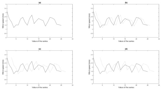
Figure 4.
Autocorrelation between the series (continuous line) and a shifted version of the series (dotted line): (a) lag 0, (b) lag 1, (c) lag 2, (d) lag 3.
As expressed before, the autocorrelation takes into account the correlation between a series and a shifted version of it. Consequently, the order of calculations to be determined is given on one hand by the number of locations and on the other by the number of time delays that are considered. Therefore, the number of operations is , so when a series is related to itself, it is only necessary to calculate the elements of the main diagonal, being necessary to multiply this number by the number of delays considered in the calculations.
- (c)
- Temporal correlation: Cross-correlation
Cross-correlation, , measures the similarity of a variable with a time-shifted version of the variable , given by Equation (15) [21]:
where is the variable at position .
Figure 5 presents an example of a short sequence, where different situations can be seen that can occur when considering a time-shifted version series over another series are shown.
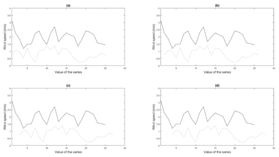
Figure 5.
Cross-correlation between the series (continuous line) and a shifted version of the series (dotted line): (a) lag 0, (b) lag 1, (c) lag 2, (d) lag 3.
As stated before, the cross-correlation expresses the correlation of a sequence with a displaced version of another one. As a consequence, the order of calculations is influenced on one hand by the number of locations and on the other by the number of temporary delays that are taken into account. Therefore, the number of operations is . When relating one series with another, it is necessary to calculate the elements outside of the main diagonal. In contrast to the spatial correlations, there is no symmetry when considering the displacement of one series over another, and this makes it necessary to multiply this number by the number of lags being considered in the calculations.
2.2. Simulation
Once the behavior of the wind speed has been described for the set of locations, it can be simulated by adjusting the calculations to the results obtained in the modeling stage to reproduce the real behavior in all places. The errors found in the data collection step can be solved with certainty. Possible different situations can be simulated.
The simulation stage is divided into five steps, developed sequentially until the results satisfy given tolerance values. These steps are described in the following sections.
2.2.1. Generation of Normal (0,1) Random Sequences
Certain values are omitted in the modeling stage because of the errors presented. To obtain the behavior of the series, the first step in the simulation is to generate random Normal (0,1) distributed series with the desired length, one for each location.
The wind speeds were considered to be distributed according to a Weibull law. However, the generated values belong to a standardized Normal distribution due to what has been explained previously. In consequence, in order to avoid unnecessary steps and possible rounding errors due to the transformations, the data generated are Normal (0,1) with a desired period of time for each studied location, i.e., to simulate a year of ten-minute periods, 52,560 values must be generated m times, where m the number of sites considered.
2.2.2. Obtaining Correlations from Random Normal (0,1) Series
The correlated sequences can be obtained from the randomly generated ones. To achieve this, it is only necessary to solve a linear system, such as the one represented in Equation (16), due to the nature of the distributions used, i.e., standardized Normal [20]:
where is a unique lower triangular matrix obtained from a decomposition of the correlation matrix, is the matrix of uncorrelated random variables with Normal (0,1) distribution, and is the matrix of correlated random variables with Normal (0,1) distribution.
There are different possibilities to obtain the unique lower triangular decomposition of the correlation matrix , that make it possible to apply the method, i.e., QR or Gaussian methods. However, has some particularities. It is symmetric and positive semidefinite, so the method to be used is the Cholesky decomposition, where the calculations of terms of matrix are given by Equation (17). This is a less computationally expensive method than the previous ones [32]:
where and correspond to each coefficient of the matrix .
By denoting the number of locations that are taken into account as and by considering the number of sums, subtractions, products, divisions, and roots necessary to determine each of the aforementioned decompositions, the Gaussian method needs operations, the QR dependent on Householder decomposition needs , and the Cholesky one uses [32].
Furthermore, the fact of applying this decomposition to the correlation matrix also offers the possibility of quickly and easily getting a solution of the correlated random series closer to the real ones, as long as the distribution is a standardized Normal, with which it can be ensured that the solution also has a standardized Normal distribution. Otherwise, keeping the desired distribution cannot be ensured [18].
2.2.3. Approximation Normal (0,1) to Weibull
As in Section 2.1.4, the transformation can be obtained by matching both CDFs, finding, as can be seen in Equation (18), instead of , with the use of c and k factors corresponding to each location:
where is the error function, defined in Equation (6).
2.2.4. Calculation of the Data Deviation
The calculation of the correlated random series with (16) does not give the desired result yet. There is some difference, and to assess it, the error given by the metric expressed in (19) has been defined. This error is based on the Euclidean norm and has been established as an objective function, a value that should be minimized. The result is a reference value that reflects how far the simulated series are from the original data [32]:
where corresponds to each component of the correlation vector obtained in the modeling stage, corresponds to each component of the correlation vector obtained in the simulation stage, and is the number of correlations calculated, considering both spatial and temporal correlations.
2.2.5. Implementation of an Evolutionary Algorithm
As mentioned in the previous step, the objective function given by Equation (19) must be minimized so that the simulated sequences satisfy the required constraints. Therefore, an evolutionary algorithm is performed that evolves until reaching the desired solution with a degree of tolerance that is small enough to make it possible to consider deviations in calculations negligible.
At each iteration, pairs of wind speed values corresponding to the sequence of one of the locations are swapped during the evolution of the algorithm. From this swapping process, the correlations are recalculated, and with an acceptance algorithm, the decision is made regarding whether or not the solutions obtained are better than the previous ones. The change is accepted when the objective function decreases and is rejected otherwise. Finally, the calculated values in the iterations are transformed from Normal (0,1) to Weibull.
The series is finally rearranged, and as the values have not been modified, the distribution features are kept in each location [20].
3. Case Study
The accuracy of the model and, consequently, of the simulation of the random data requires a good set of the necessary parameters. The framework of the results obtained in this paper is Galicia, the autonomous region located in the Northwest of Spain because this is one of the areas where wind energy has a greater potential. In fact, in 2019, Galician wind farms presented the third part of the total installed power in the region, exceeding the combination of conventional sources [33], with a total number of 4026 wind turbines installed [34].
A large amount of the wind power installed in Galicia is located in the northeast of the region, and due to this, the study places belong to this area. From the meteorological stations of the MeteoGalicia network [35], the data from the Fragavella, Labrada and Lanzós stations corresponding to 2019 were selected. Once the locations to be considered in the study are known, the data collected are the wind speeds of each location. With them, it is possible to analyze the simultaneity, and as the height at which they were collected is known, this makes it possible to calculate the wind speeds at the study height. One of the objectives of this study is to determine the relationship between distances and correlations. Therefore, based on the coordinates of the meteorological stations, the straight line distance between each pair of locations was obtained. In Figure 6, the positions of the selected places and their distances in km are shown.
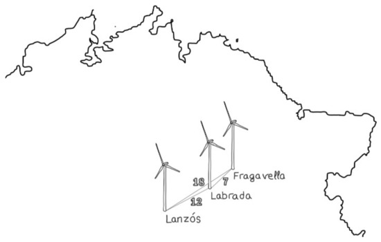
Figure 6.
Selected locations and distances between them.
The data collection height of the selected meteorological stations is different from the height of wind turbine hubs, i.e., the height of the study of the simultaneity of wind speeds. Therefore, it is necessary to characterize the friction factor of the terrain for each of the selected sites. In Table 1, the estimated friction factors and the different data heights available at the MeteoGalicia website are shown.

Table 1.
Friction factor of the terrain and meteorological station height in each location.
By analyzing the frequency of the wind speeds in the collected data, it is possible to affirm that the trend of the wind speed in all those locations is correctly described by the Weibull distribution. The shape and scale parameters of each location are calculated using Equations (3) and (4), and the results are shown in Table 2.
Table 2.
Weibull parameters for each of the studied locations.
4. Results
The development of the method presented in the previous sections allows improving the knowledge of the behavior of the simultaneous wind speeds in different locations, obtaining correlated series of random wind speeds through a model where the influence of each location on the group is assessed. The steps of the method are directly applied through the use of the equations presented and, therefore, its potential is evaluated in different scenarios to assess its scope and applicability. The scenarios are The variation of the data collection or simulation period; the arrangement of a different number of locations; and determining the influence of the distance in the correlations, or the calculation time and the number of iterations necessary to obtain the results with a marked tolerance. Finally, the results can be extrapolated for the consideration of a greater number of places. To achieve the calculation times and the number of iterations required in the group of locations, a computer with an i7 950 processor and 24 GB of RAM is used, and tolerance of 0.05 is defined.
4.1. Modeling
Once a decision about the locations to be investigated has been made, the first phase of the algorithm is carried out, i.e., the simultaneity is obtained. The next parts show the results obtained with the analysis, considering 2 or 3 places and increasing the data collection period or considering a greater number of locations.
4.1.1. Two Locations Relationship
In the first case performed during the modeling phase, the behavior of the wind speed in two locations is evaluated. The calculation time of the algorithm until the correlations are reached is 0.60 s in the case of Fragavella and Labrada and 0.59 s in the case of Fragavella and Lanzós. The difference in the computation time between both studies is practically negligible, and, initially, there does not seem to be any relationship between distance and calculation time.
Comparing Table 3 and Table 4, the spatial correlations and cross-correlations have remarkably high values between Fragavella and Labrada and exceptionally low between Fragavella and Lanzós. Therefore, it can be deduced that the distance between the places influences the correlations inversely, i.e., the greater the distance is, the lower the correlations are and vice versa. On the other hand, the values of the autocorrelations in both cases are exceedingly high, and thus, it can be deduced that there is a temporal influence among the values of the series in each of the locations.
Table 3.
Obtained correlations in the modeling stage for the study with Fragavella, 1, and Labrada, 2.
Table 4.
Obtained correlations in the modeling stage for the study with Fragavella, 1, and Lanzós, 3.
4.1.2. The Case of Three Locations
Once obtained the wind speed correlations for two locations, the behavior of the algorithm is evaluated for three places. In this case, the algorithm calculation time in the modeling stage is 1.48 s, which, even though still being low, corresponds to a large increase concerning the previous cases. In Table 5, it can be seen that the spatial correlations and cross-correlations have remarkably high values between Fragavella and Labrada and exceptionally low between Fragavella and Lanzós. On the other hand, the correlations between Labrada and Lanzós continue to have reduced values, not as much as between Fragavella and Lanzós, as was expected from the derivation of the inverse relationship between distance and correlations. Moreover, there is a temporal influence between the values of the series in each of the locations since autocorrelations have high values. Furthermore, comparing the results with Table 3 and Table 4, the values of the correlations between pairs are kept.
Table 5.
Obtained correlations in the modeling stage for the study with Fragavella, 1, Labrada, 2, and Lanzós, 3.
4.1.3. Variation of Time Interval Length
In the previous sections, a data collection period of 1 year was used. However, this may change since the previous measurement campaign duration might have been different. In this section, the influence of duration periods on the algorithm is assessed.
Therefore, the influence on the results was evaluated for a data collection period of 5 years, from 2015 to 2019. This longer data length involves an increased number of measurement errors corresponding to each of the sites and, in turn, a larger calculation time. However, since these data are only used in the modeling phase, the influence on the calculation time is reduced. Thus, the algorithm is practically straightforward in the modeling stage, with a calculation time lower than 1 s in the case of 3 locations and one year of data and around 4 s for the case of 5 years.
The results obtained for 1 or 5 years should not differ if the resource is well characterized. To confirm this, the Weibull parameters and the correlations are calculated using Equations (3) and (4) and are shown in Table 6 and Table 7, respectively.
Table 6.
Weibull parameters for each of the studied locations for a period of 5 years.
Table 7.
Correlations obtained in the modeling stage for the study with Fragavella, 1, Labrada, 2, and Lanzós, 3, for a period of 5 years.
4.1.4. Higher Number of Locations
The last step in the modeling stage is to verify the influence of a superior number of locations, . The order of operations that are needed to calculate each of the correlations was determined and shown in Table 8 since the rest of the executions are not time-consuming.
Table 8.
Order of necessary operations during the modeling stage.
Taking into account the previous values and the characteristics of the computer used, the evolution of the calculation time in the modeling stage is determined by increasing the number of locations, Figure 7.
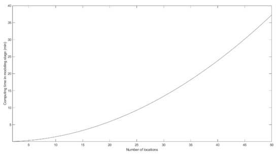
Figure 7.
Evolution of the calculation time required to carry out the modeling stage considering a different number of locations.
Looking at Figure 7, it can be checked that the calculation time of the modeling stage grows with the number of locations, so in a scant number of places, the time needed to reach a result is practically null, as it was said in previous sections, of about 0.6 s for 2 sites or of about 1.5 s for 3. As the number of locations increases, the calculation time rises, and it reaches about 37 min when 50 places are being evaluated. As can be seen in Table 8, this is due to the fact that the number of calculations increases in a quadratic order with the number of locations and, as a consequence, so do the number of operations to be carried out in the modeling stage.
4.2. Simulation
When the simultaneity characteristics between places have been analyzed, random wind speeds are generated for a period, mainly of one year. The following sections show the results obtained in the simulations effectuated, considering 2 or 3 places, increasing the data collection period, or considering a greater number of locations.
4.2.1. Two Locations Relationship
Such as in the modeling stage, in the first analysis performed, the behavior of wind speeds in two locations is evaluated. The calculation time of the algorithm until the tolerance is reached is 22 h and 3.35 min in 2,599,096 iterations in the case of Fragavella and Labrada and 16 h and 36.59 min in 2,231,562 iterations in the case of Fragavella and Lanzós, existing significant differences in the computation times and iterations between both studies. On the other hand, it can be verified that the calculation times are higher in the modeling stage than in simulation one, corresponding to some hours in the simulation concerning a few seconds in the modeling.
As can be seen in Figure 8, the initial data deviation concerning the tolerance marked in the study with Fragavella and Labrada is higher than that with Fragavella and Lanzós and, consequently, the calculation time period is higher, unlike in the case of the modeling, where the times were practically identical. However, the behavior of the data deviation between the required solution and the calculated one varies in a similar way along the time, so in both cases, there is a period with a rapid decrease, up to 4 h in the case of Fragavella and Labrada and up to 3 h in the case of Fragavella and Lanzós, after which the refinement to the required solution slows down.
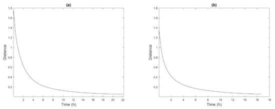
Figure 8.
Evolution of the data deviation to the real solution through time in the simulation stage: (a) study considering Fragavella and Labrada, (b) study considering Fragavella and Lanzós.
Table 9 and Table 10 show the results obtained for the correlations of the simulation phase in each of the analyses performed. Observing their values and comparing them with Table 3 and Table 4, it can be deduced that the method used to correlate the random series given by Equation (16) has a result that is very close to the solution considering just the spatial correlations. This is mainly because the method used to correlate the series is the Cholesky decomposition of the spatial correlation matrix. However, the values of the temporal correlations are close to 0 because the series was randomly generated. On the other hand, it can be verified that there is a very good accuracy of the iterative algorithm, so the solutions are very close to the objective, with differences lower than 5% in each of the cases.
Table 9.
Obtained correlations in the simulation stage for the study with Fragavella, 1, and Labrada, 2.
Table 10.
Obtained correlations in the simulation stage for the study with Fragavella, 1, and Lanzós, 3.
4.2.2. Three Locations Relationship
Once obtained the wind speed correlations for two locations, the behavior of the algorithm is evaluated for the case of three places. In this case, the algorithm calculation time in the simulation stage is 1 day, 23 h and 15.53 min in 3,999,039 iterations. As before, the calculation time in the simulation stage is much higher than the respective in the modeling stage, and, as occurs in the analysis of 3 locations in the modeling phase, the computation time is larger than in the case of 2 places.
As can be seen in Figure 9, the behavior of the data deviation between the required solution and the calculated one in each iteration along the time is similar to that previously studied in the case of 2 sites, a few hours with a fast decrease in this case, up to 8 h, and then a refinement of the solution to the marked tolerance. On the other hand, comparing it with Figure 8, it can be seen that the initial solution is further away from the desired one in the case of 3 sites concerning any of the studies of 2 locations, this having an impact on both the calculation time and the number of iterations required to achieve the desired values.
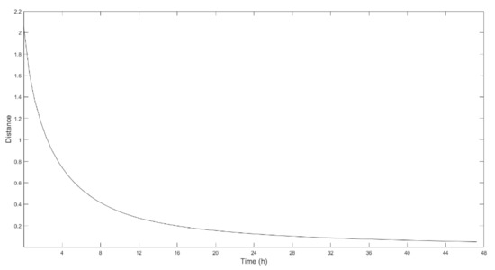
Figure 9.
Evolution of the data deviation to the real solution through time in the simulation stage with the consideration of the locations of Fragavella, Labrada and Lanzós.
Table 11 shows the results of the correlations obtained with the application of the proposed algorithm for 3 locations. Like before, after the random series correlation given by Equation (16), the spatial correlations are very close to those corresponding to the objective solution. However, the temporal ones are around the value 0. The algorithm remains very precise with the consideration of 3 sites, so the differences between the objective results and those obtained with the simulation are lower than 5% in each of the cases.
Table 11.
Correlations obtained in the simulation stage for the study performed between Fragavella, 1, Labrada, 2, and Lanzós, 3.
4.2.3. Variation of the Time Interval Length
In the previous sections, a simulated data generation period of one year was considered. However, dealing with a different period of time can be of interest. In this section, the influence of different intervals of data is estimated.
This was evaluated for a shorter period of generation of simulated values. It was checked for half a year and for two years. As expected, the greater amount of data influences the performance of the code, taking on average more than twice the time to perform an iteration, with an average of 0.1 s compared to about 0.04 s. On the other hand, a lower amount of data requires less computational time per iteration, with an average of 0.03 s instead of about 0.04 s.
In addition, as previously commented, the simulation stage is very heavy and requires long calculation periods to reach high accuracies, so performing a simulation with a greater amount of simulated values can make code take too long, going from approximately 20 h to practically 2 days of calculation time in the case of 2 sites, or from around 2 days up to 4 of computing time in the case of 3 locations. However, the reduction in the number of values can lighten the code time, requiring about 16 h instead of 20 h in the case of 2 places, or one day and about 20 h instead of practically 2 days in the case of 3 sites.
On the other hand, the trends of the correlations remain, so there are values very close to the spatial correlations and around 0 in the temporal correlations after the resolution of the system by the Cholesky decomposition, and values with an error lower than 5% in each of the correlations obtained after the iterative algorithm.
4.2.4. Higher Number of Locations
As in the modeling phase, the last step in the simulation phase is to confirm the influence of a greater number of sites. To take into account a different number of locations, the order of operations needed for the calculation of each of the correlations and the Cholesky decomposition, Table 12, was determined since the rest of the executions are practically instantaneous. It must be taken into account that the Cholesky decomposition is only performed once to correlate the random series generated.
Table 12.
Order of operations needed in the simulation stage.
Considering the previous values and the characteristics of the computer used, it was determined how the calculation time evolves by iteration of the simulation stage by the number of sites, Figure 10.
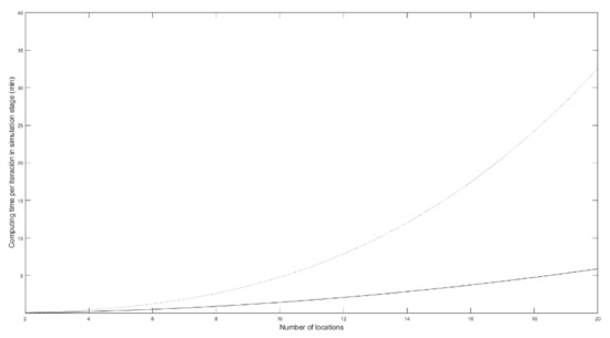
Figure 10.
Evolution of the calculation time required to carry out each iteration of the simulation stage considering a different number of locations, where the dotted line corresponds to the first iteration and the solid line to the rest of iterations.
In Figure 10, it can be seen that the calculation time of the first iteration of the simulation phase grows much faster than the rest of the iterations, considering the number of places following the values in Table 12. This is because in the first iteration, the calculation by the Cholesky method must be performed, with a cubic growth concerning a quadratic one.
By using the conclusions obtained in the previous sections, as the number of locations increases, the desired solution is further away, requiring a greater number of iterations, so, following the data in Table 12, the amount of correlations close to the desired solution after applying the Cholesky method, that is, the spatial ones, is . On the other hand, the amount of correlations far from the desired solution, that is, the temporal ones are . The latter is growing faster than the former.
5. Conclusions
The growing trend of incorporating wind energy into electric power networks makes its characterization a mathematical problem. The inherent uncertainty due to errors made during the data collection process, together with the unpredictability nature of wind speed, makes it difficult to accurately obtain the power to be injected into the network at each moment. The simulation of wind speed series with a certain degree of accuracy can be carried out after obtaining the models of the behavior of each location and the relationships among them through the calculation of the spatial and temporal correlations.
The method presented in this paper is intended to deal with the errors that occur in the data collection period in which a wind speed value is either unknown or known, but its reliability cannot be assessed. By calculating the spatial correlations, it is possible to identify the trends of the wind speeds for the set of locations. If temporal correlations are also considered, it is possible to characterize the wind speeds in different time intervals.
By simulating random values, it is possible to characterize the wind speed in different periods or stages. The simulation makes it possible to cover the gaps that arise due to the lack of knowledge of the wind speeds and also to estimate the values that can occur in subsequent periods of time. This facilitates knowing the power injected into the electrical network with a certain degree of reliability. Additionally, the accuracy of the method is as close to reality as desired when a level of tolerance is established. In this work, a value of 0.05 is considered reduced enough. As a result, errors are lower than 5% in all simulated cases.
The data used in this paper correspond to 2019 in the meteorological stations of Fragavella, Labrada and Lanzós, all of them selected from the MeteoGalicia website. The wind speeds are considered to fit Weibull distributions. It was verified that the studied locations meet this assumption.
There seems to be an inverse relationship between distance and correlation. When the distance between locations is high, the calculation time is shorter because the Cholesky decomposition initializes the iterative algorithm closer to the solution, so the number of iterations is low.
The consideration of a higher number of locations directly affects the calculation time. On one hand, a large number of operations per iteration is needed, having to perform calculations, where m is the number of locations, and on the other, the solution of the correlated series obtained before Cholesky decomposition is increasingly far from the objective because values corresponding to the temporal correlations increases more rapid, , then the spatial correlations, , which can influence the number of iterations required, making the problem with a large number of locations become unapproachable.
The modeling stage, where the relationships between locations are reproduced, is practically instantaneous, with a duration of a few seconds. Nevertheless, the simulation stage, where the randomness of the wind speed is reproduced, is more time-computing, reaching several hours in some cases. Moreover, on one hand, the variation of the collection data period does not involve a significant time. On the other, the number of simulated values affects the calculation time, and this can make the problem unapproachable in the case of the simulation of a large one.
Author Contributions
Conceptualization, M.C.-C. and D.V.; methodology, M.C.-C. and D.V.; software, M.C.-C.; validation, M.C.-C. and J.M.-T.; formal analysis, M.C.-C. and A.E.F.-L.; investigation, M.C.-C. and D.V.; resources, D.V. and A.E.F.-L.; writing—original draft preparation, M.C.-C.; writing—review and editing, A.E.F.-L. and J.M.-T.; visualization, D.V.; supervision, D.V. and A.E.F.-L.; project administration, A.E.F.-L. and J.M.-T.; funding acquisition, D.V. and A.E.F.-L. All authors have read and agreed to the published version of the manuscript.
Funding
This research received no external funding.
Institutional Review Board Statement
Not applicable.
Informed Consent Statement
Not applicable.
Data Availability Statement
Not applicable.
Conflicts of Interest
The authors declare no conflict of interest.
References
- Xu, X.; Xiao, B.; Li, C.Z. Critical factors of electricity consumption in residential buildings: An analysis from the point of occupant characteristics view. J. Clean. Prod. 2020, 256, 120423. [Google Scholar] [CrossRef]
- Handayani, Y.; Krozer, Y.; Filatova, T. From fossil fuels to renewables: An analysis of long–term scenarios considering technological learning. Energy Policy 2019, 127, 134–146. [Google Scholar] [CrossRef]
- Sayed, E.T.; Wilberforce, T.; Elsaid, K.; Rabaia, M.K.H.; Abdelhareem, M.A.; Chae, K.J.; Olabi, A.G. A critical review on environmental impacts of renewable energy systems and mitigation strategies: Wind, hydro, biomass and geothermal. Sci. Total Environ. 2021, 766, 144505. [Google Scholar] [CrossRef] [PubMed]
- United Nations Climate Change. Paris Agreement; United Nations: France, Paris, 2015. [Google Scholar]
- Directorate General for Energy. Energy Roadmap 2050; European Commission: Luxembourg, 2012. [Google Scholar]
- Tovar–Facio, J.; Martín, M.; Ponce–Ortega, J.M. Sustainable energy transition: Modeling and optimization. Curr. Opin. Chem. Eng. 2021, 31, 100661. [Google Scholar] [CrossRef]
- Wind Europe. Wind Energy and Economic Recovery in Europe; Wood Mackenzie: Edinburgh, UK, 2020. [Google Scholar]
- Jung, D.W. Design improvement and manufacturing of nacelle cover for wind turbine. Int. J. Mech. Eng. Robot. Res. 2020, 9, 177–183. [Google Scholar] [CrossRef]
- Nazir, M.S.; Alturise, F.; Alshmrany, S.; Nazir, H.M.J.; Bilal, M.; Abdalla, A.N.; Sanjeevikumar, P. Wind generation forecasting methods and proliferation of artificial neural network: A review of five years research trend. Sustainability 2020, 12, 3778. [Google Scholar] [CrossRef]
- Villanueva, D.; Feijóo, A.; Pazos, J.L. Multivariate Weibull distribution for wind speed and wind power behaviour assessment. Resources 2013, 2, 370–384. [Google Scholar] [CrossRef]
- Hicham, B.; El Abbassi, I.; El Bouardi, A.; Darcherif, A. Wind speed data analysis using Weibull and Rayleigh distribution functions, case study: Five cities Northern Morocco. Procedia Manuf. 2019, 32, 786–793. [Google Scholar]
- Guenoukpati, A.; Salami, A.A.; Kodjo, M.K.; Napo, K. Estimating Weibull parameters for wind energy applications using seven numerical methods: Case studies of three coastal sites in West Africa. Int. J. Renew. Energy Dev. 2020, 9, 217–226. [Google Scholar] [CrossRef]
- Tian, Z.; Li, H.; Li, F. A combination forecasting model of wind speed based on decomposition. Energy Rep. 2021, 7, 1217–1233. [Google Scholar] [CrossRef]
- Abedinia, O.; Lofti, M.; Bagheri, M.; Shafie-Khah, B.; Catalao, J.P.S. Improved EMD-Based complex prediction model for wind power forecasting. IEEE Trans. Sustain. Energy 2020, 11, 2790–2802. [Google Scholar] [CrossRef]
- Bañuelos–Ruedas, F.; Angeles–Camacho, C.; Rios–Marcuello, S. Analysis and validation of the methodology used in the extrapolation wind speed data at different heights. Renew. Sustain. Energy Rev. 2010, 14, 2383–2391. [Google Scholar] [CrossRef]
- Ti, Z.L.; Li, Y.L.; Liao, H.L. Effect of ground surface roughness on wind field over bridge site with a gorge in mountainous area. Gongcheng Lixue/Eng. Mech. 2017, 34, 73–81. [Google Scholar]
- Afandi, A.N.; Fadlika, I.; Gumilar, L.; Hiyama, T. Wind gradient impact on the potential wind energy profile based on the ground launch. In Proceedings of the 3rd International Seminar on Metallurgy and Materials, Tangerand Selatan, Indonesia, 23–24 October 2019; Volume 2228. [Google Scholar] [CrossRef]
- Villanueva, D.; Feijóo, A.; Pazos, J.L. Simulation of correlated wind speed data for economic dispatch evaluation. IEEE Trans. Sustain. Energy 2012, 3, 142–149. [Google Scholar] [CrossRef]
- Appino, R.R.; González Ordiano, J.Á.; Mikut, R.; Faulwasser, T.; Hagenmeyer, V. On the use of probabilistic forecasts in scheduling of renewable energy sources coupled to storages. Appl. Energy 2018, 210, 1207–1218. [Google Scholar] [CrossRef]
- Foley, A.M.; Leahy, P.G.; Marvuglia, A.; MCKeogh, E.J. Current methods and advances in forecasting wind power generation. Renew. Energy 2012, 37, 1–8. [Google Scholar] [CrossRef]
- Feijóo, A.; Villanueva, D.; Pazos, J.L.; Sobolewski, R. Simulation of correlated wind speeds: A review. Renew. Sustain. Energy Rev. 2011, 15, 2826–2832. [Google Scholar] [CrossRef]
- Nuño Martínez, E.; Cutululis, N.; Sørensen, P. High dimensional dependence in power systems: A review. Renew. Sustain. Energy Rev. 2018, 94, 197–213. [Google Scholar] [CrossRef]
- Deng, J.; Li, H.; Hu, J.; Liu, Z. A new wind speed scenario generation method based on spatiotemporal dependency structure. Renew. Energy 2021, 163, 1951–1962. [Google Scholar] [CrossRef]
- Kaplan, O.; Temiz, M. A novel method based on Weibull distribution for short–term wind speed prediction. Int. J. Hydrog. Energy 2017, 42, 17793–17800. [Google Scholar] [CrossRef]
- Hu, J.X.; Li, H.R. A new clustering approach for scenario reduction in multi–stochastic variable programming. IEEE Trans. Power Syst. 2019, 34, 3813–3825. [Google Scholar] [CrossRef]
- Valizadeh Haghi, H.; Lotfifard, S. Spatiotemporal modelling of wind generation for optimal energy storage sizing. IEEE Trans. Sustain. Energy 2015, 6, 113–121. [Google Scholar] [CrossRef]
- Malvaldi, A.; Weiss, S.; Infield, D.; Browell, J.; Leahy, P.; Foley, A.M. A spatial and temporal correlation analysis of aggregate wind power in an ideally interconnected Europe. Wind Energy 2017, 20, 1315–1329. [Google Scholar] [CrossRef]
- Morales, J.M.; Mínguez, R.; Conejo, A.J. A methodology to generate statistically dependent wind speed scenarios. Appl. Energy 2010, 87, 843–855. [Google Scholar] [CrossRef]
- Measnet. Evaluations of Site-Specific Wind Conditions; Measnet: Madrid, Spain, 2016. [Google Scholar]
- Martín, C.M.S.; Lundquist, J.K.; Clifton, A.; Poulos, G.S.; Scjreck, S.J. Wind turbine power production and anual energy production dependo n atmospheric stability and turbulence. Wind Energy Sci. 2016, 1, 221–236. [Google Scholar] [CrossRef]
- Teng, L.; Ehrhardt, M.; Günter, M. Modelling stochastic correlation. J. Math. Ind. 2016, 6. [Google Scholar] [CrossRef]
- Epperson, J.F. An Introduction to Numerical Methods and Analysis; John Wiley & Sons: Hoboken, NJ, USA, 2013. [Google Scholar]
- INEGA. Potencia Eléctrica Instalada en Galicia. Available online: http://www.inega.gal/sites/default/descargas/enerxia_galicia/potencia_electrica_castellano.pdf (accessed on 22 January 2021).
- AEE. Mapa de Parques Eólicos. Available online: www.aeeolica.org/sobre-la-eolica/la-eolica-espana/mapa-de-parques-eolicos (accessed on 22 January 2021).
- MeteoGalicia. Lista de Estaciones. Available online: www.meteogalicia.gal/observacion/rede/redeIndex.action?request_locale=es (accessed on 22 January 2021).


Publisher’s Note: MDPI stays neutral with regard to jurisdictional claims in published maps and institutional affiliations. |
© 2021 by the authors. Licensee MDPI, Basel, Switzerland. This article is an open access article distributed under the terms and conditions of the Creative Commons Attribution (CC BY) license (https://creativecommons.org/licenses/by/4.0/).