Pitch Angle Optimization for Small Wind Turbines Based on a Hierarchical Fuzzy-PID Controller and Anticipated Wind Speed Measurement

Abstract

Wind energy is an alternative to meet the growing energy demand and protect the environment; however, in places with limited wind resources, only the installation of small horizontal-axis wind turbines (SHAWTs) is profitable. At the height of these turbines, the wind is usually unstable with gusts and turbulence due to obstacles in its path such as buildings and trees. The pitch angle must be adaptable to guarantee nominal rotation speed, and it is commonly regulated with a proportional-integral-derivative (PID) feedback controller. This controller works well when the wind is stable, but not with drastic changes in wind speed. To correct this problem, this article introduces a PID controller with automatic adjustment of the gain values using a fuzzy logic controller (FLC). The PID gain adjustment allows an optimal response speed of the system for different wind conditions. The membership functions of the FLC are determined from a methodology that includes: The measurement of the wind speed at a calculated distance, a statistical analysis of the wind variability, and a dynamic analysis of the wind path. In this way, it is possible to anticipate the response of the actuator to the arrival of a gust of wind to the rotor. The algorithm is implemented in 14 kW SHAWTs where the difference in performance with a conventional controller is quantified. Satisfactory results were obtained, the electrical output increased by 7%, and the risk of rotor damage due to vibrations or mechanical fatigue was reduced by 20%.

1. Introduction

The generation of large amounts of electricity is necessary to meet the growing demand; generating it through natural renewable resources is essential for the care of the environment. Within clean energy, wind energy has had great momentum in recent years. The Global Wind Energy Council reported 60.4 GW of new installations in 2019, and a global capacity of 651 GW and an expectation of growth of more than 100 GW in annual installations over the next decade [1]. However, the technological trend points to the development and construction of increasingly large wind turbines. Currently, the highest-capacity wind turbine is produced by Siemens Gamesa that generates 14 MW of nominal power, has a swept area diameter of 222 m, and requires an annual average wind speed of 10 m/s [2].

In places with lower wind resources, it is necessary to install small horizontal-axis wind turbines (SHAWTs). IEC 61400-1: 2014 defines “small wind turbines” as those with a swept area less than 200 m² and generation voltage less than 1000 V AC or 1500 V DC [3]. SHAWTs require a cut-in wind speed of 4 m/s [4]. Fifty percent of the planet has an average wind speed greater than 6.04 m/s at a height of 10 m [5]. These areas include buildings, trees, or mountains that are obstacles to the wind path, causing a decrease in wind speed and an increase in turbulence. The turbulence area reaches 2 or 3 times the height of the obstacles, while in the frontal contact part, it is 2 to 10 times [6].

Disorderly wind motion and fluctuating wind speed magnitude hinder the efficiency of a wind turbine and can be prone to failures, even catastrophic ones [7]. Therefore, a wind turbine should operate with variable wind speed and regulate the effect of the wind force on the rotor by controlling the angle of incidence between the blade and the wind flow [8]. The classical method of pitch angle control is the proportional integral derivative (PID), which is based on a mathematical model of the system with feedback of the controlled variable, as it calculates the error between the measured and desired values [9]. To adjust the controller, the weights of the proportional constant, the integral time, and the derivative time (gains) are determined [10]. This adjustment of optimum values of gains is performed for the desired control response. However, in a variable-speed wind turbine, the optimal response changes as a function of the magnitude of the wind speed variation. This variability makes a PID controller unstable with drastic changes in the wind speed [11,12].

Pitch control methods in a wind turbine that mitigate changes in wind speed were found in the literature reviewed. In [13,14,15], a fuzzy logic controller (FLC) selects the previously calculated PID gains for the negative or positive error of the process variable, or if the error is very large. In [16], an artificial neural network determines the PID gain values. In [17], the “differential evolution” optimization algorithm is used to change the PID gain values as the operating point changes. In [18,19], the proportional and integral gains of a proportional integral (PI) controller are adjusted by a “particle swarm” optimization algorithm. In [20], a “flame-moth” optimization algorithm is proposed, the candidate solutions are moths, and the PID parameters are the position of the moths in a 3D search space. In [11], an optimization algorithm based on the teaching-learning model of a classroom is used to calculate the gains of a PI controller. These known methods have different disadvantages. They improve the response of the control signal for different wind speed ranges, as the controller is adjusted for each of these ranges. However, when there is a sudden change in wind speed, the response of the controller is not optimal, due to the inertial impulse generated in the rotor. If the gain tuning is done using a search algorithm or neural networks, the global optimum solution is not guaranteed, because it can be set to a local minimum/maximum solution. These methods are limited by the mechanical rotational speed of the pitch angle; even if the optimal control signal response is obtained, it is not possible to obtain the optimal pitch angle position.

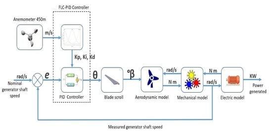
This paper proposes an innovative PID controller with automatic adjustment of its gains by means of an FLC. Unlike the proposed methods, the membership functions of the FLC are determined based on two criteria. The first criterion is to monitor the error of the controlled variable, which is the generator shaft speed and the magnitude of the change in this error. The second criterion is related to drastic changes in wind speed. An anemometer is installed at a certain distance that allows the controller to anticipate the pitch angle change before receiving the wind impact on the rotor. This ensures an anticipated response in the position of the angle of incidence and avoids an excessive rotational speed of the turbine, which increases the efficiency and safety of the system. In addition, the methodology proposes a statistical analysis of the historical wind behavior to determine the values of stable and gust wind speed. With this information, the global optimal values of the PID controller gains are determined.

Therefore, this work contributes scientifically with a methodology for the development of a PID-FLC control algorithm for the pitch angle in a SHAWT. This algorithm solves the problem of controlling a nonlinear system due to wind randomness. The research question or hypothesis is to determine that it is possible to increase the performance of a SHAWT using a PID-FLC controller, compared to a classical PID controller. In this way, this research helps SHAWT users to improve their system, increasing their energy production and reducing maintenance costs.

The article is structured by initially presenting the methodology of the algorithm development. The methodology proposes to set the operating limits of the wind turbine using its mathematical model, perform a statistical analysis of the wind to determine its variability, calculate the distance between the installation site of the anemometer and the turbine, validate the location of the anemometer using a dynamic analysis of the wind trajectory, determine the domain of the PID gain values, and assign the FLC rules. The validation of the proposed PID-FLC control algorithm is performed by simulation. A series of staggered pulses with different amplitude values are considered input variables. Each pulse represents different wind speed conditions, which test the response and reliability of the algorithm. Finally, the results of the implementation of the algorithm on a three-bladed SHAWT with a swept area of 130 m² and a 14 kW permanent magnet synchronous generator (PMSG) are presented. A comparison between the conventional and the proposed PID controller is performed to quantify the differences in their performance and to test the hypothesis.

2. Materials and Methods

To develop the proposed algorithm, it is necessary to follow a methodology that is the conceptual support that governs the way we use the information. Knowing the physical specifications of the SHAWT is the first step. The mathematical model of the SHAWT system is developed to determine the initial values of the PID controller, as well as the aerodynamic limits. Statistical analysis is developed to determine the variability in the wind, the magnitude of the change in the wind speed, and the recurrent wind speed, as well as the prevailing direction. The speed of the pitch angle mechanical system determines the distance from the wind turbine to the anemometer. A dynamic analysis of the wind behavior validates the location of the anemometer and reduces errors in the mediation due to disturbances in the wind path toward the rotor. Finally, with this information, the membership functions of the FLC controller that adjust the gains of the PID controller are proposed.

The SHAWT used consists of three blades, 6.4 m long and 1.2 m at its widest part, made of fiberglass and polyester with a weight of 260 kg each. The aerodynamic design is a NACA-6812. The height of the hub is 18 m. The system has a gearbox with a ratio of 1:2.1 and a 14 kW PMSG with a nominal speed of 14.6 rad/s.

Table 1. PMSG specifications.

Power	14 kW	Apparent power	14.3 kVA
Phases	3	Frequency	20.3 Hz
Volts AC	385 V	Power factor	0.945
Amps AC	22.2 A	Insulation class	H
Revolutions per minute	135	Service	Continuous
Frame	TC5V	Maximum temperature	80 °C
IP Class	IP32	Weight (kg)	650

shows the generator specifications.

The SHAWT is in the Autonomous University of Queretaro, Mexico, at an altitude of 1969 m. Figure 1 shows the SHAWT used; this image was taken by the authors.

2.1. Mathematical Model

SHAWT’s mathematical model is developed by three blocks, the rotor aerodynamics, the mechanical system, and the PMSG.

In the aerodynamic model, the wind energy that turns the rotor is calculated. The wind power is described in Equation (1) [21]. (The symbols used in each of the equations are defined in the nomenclature at the end of the paper.)

$$P_{rotor}=\frac{1}{2}\rho A V^3 Cp$$

(1)

Cp is obtained experimentally for values 3 < λ < 15, presented in Equation (2) [22].

$$Cp=\left({\displaystyle \sum }_{i=0}^4{\displaystyle \sum }_{j=0}^4{\alpha }_{i,j}{\beta }^j{\lambda }^i\right)$$

(2)

λ is obtained by Equation (3) [22] and values of α_i,j are presented in

Table 2. Coefficients α_i,j for Cp calculation [22].

i	j	αi,j	i	j	αi,j
4	4	4.9686 × 10−10	4	3	−7.1535 × 10−8
4	2	1.6167 × 10−6	4	1	−9.4839 × 10−6
4	0	1.4787 × 10−5	3	4	−8.9194 × 10−8
3	3	5.9924 × 10−6	3	2	−1.0479 × 10−4
3	1	5.7051 × 10−4	3	0	−8.6018 × 10−4
2	4	2.7937 × 10−6	2	3	−1.4855 × 10−4
2	2	2.1495 × 10−3	2	1	−1.0996 × 10−2
2	0	1.5727 × 10−2	-	-	-
1	4	−2.3895 × 10−5	1	3	1.0683 × 10−3
1	2	−1.3365 × 10−4	1	1	6.0405 × 10−2
1	0	−6.7606 × 10−2	0	4	1.1524 × 10−5
0	3	−1.3365 × 10−4	0	2	−1.2406 × 10−2
0	1	2.1808 × 10−1	0	0	−4.1909 × 10−1

.

$$\lambda =\frac{w_{rotor}R}{V}$$

(3)

The torque of the rotor is determined by Equation (4) [23].

$$T_{rotor}=\frac{1}{2}\rho \pi R^3{V}^2\frac{C_p}{\lambda }$$

(4)

The mechanical system is modeled as a system of two opposing masses, the rotor and the generator, and the rotational speeds are the resulting variables. The mathematical model is determined by Equations (4)–(6) [24].

$$\frac{d{w}_{gen}}{dt}=\frac{1}{2H_{gen}}\left[\frac{P_{elec}}{w_{gen}+w_0}-d_{rg}\left(w_{gen}-w_{rot}\right)-k_{rg}\Delta {\theta }_m\right]$$

(5)

$$\frac{d{w}_{rot}}{dt}=\frac{1}{2H_{rot}}\left[-\frac{P_{rotor}}{w_{rot}+w_0}+d_{rg}\left(w_{gen}-w_{rot}\right)+k_{rg}\Delta {\theta }_m\right]$$

(6)

$$\frac{d\left(\Delta {\theta }_m\right)}{dt}=w_{ref}\left(w_{gen}-w_{rot}\right)$$

(7)

In a two-mass system, the rotor and generator relate to an equivalent shaft stiffness k_rg, which can be determined from the parallel shaft stiffness as in (8) [24]. The generator and gearbox damping must be added together in d_rg, and the mutual damping of the gearbox and generator is neglected in the two-mass shaft model.

$$\frac{1}{k_{rg}}=\frac{1}{\left(\frac{k_{rgb}}{n_{gb}^2}\right)}+\frac{1}{k_{gbg}}$$

(8)

Inertial moments are calculated according to (9) and (10) [22].

$$H_{rotor}=\frac{J_{rotor} w_{rotor}^2}{2 P_{nom}}$$

(9)

$$H_{gen}=\frac{J_{gen} w_{gen}^2}{2 P_{nom}}$$

(10)

The inertia of the rotor is approximated with (11) [22]. The rotor mass m_r includes all blades. Generator inertia J_gen is regularly provided by the manufacturer.

$$J_{rotor}=\frac{1}{8}{m}_r{R}^2$$

(11)

A PMSG is modeled with two axes (d) and (q), out of phase by 90 electrical degrees in a synchronous rotation. The d-q stator voltages are given in (12) and (13) [23].

$$V_d=R_d{I}_d+L_d\frac{d{I}_d}{dt}-{\omega }_{gen}{L}_q{I}_q$$

(12)

$$V_q=R_q{I}_q+L_q\frac{d{I}_q}{dt}+{\omega }_{gen}\left(L_d{I}_d+{\phi }_f\right)$$

(13)

The rotational speed of the generator and the reference speed calculated for power levels below 46% are described with (14) and (15), respectively [21]. Finally, the electromechanical torque is expressed as (16) [21].

$${\omega }_{gen}=P_p{\omega }_{ref}$$

(14)

$$w_{ref}=-0.75P_{elec}^2+1.59P_{elec}+0.63$$

(15)

$$T_{gen}=\frac{3}{2}{P}_p{\omega }_{ref}\left(\left(L_q-L_d\right)i_d{i}_q+{\phi }_f{i}_q\right)$$

(16)

2.2. Statistical Wind Analysis

Statistical wind analysis in wind farm feasibility studies is determined from a sampling frequency of 1 s and averaged over 10 min intervals to represent the average wind characteristics. In addition, dispersion through standard deviation is considered. Both parameters are considered for wind speed and direction to establish its variability and to determine the dominant direction. A Weibull distribution is used to analyze the variability in wind speed [6].

Measurements should be made at a height of 10 m by using a weather tower without obstacles that disturb the air flow. Historical information should be available for as long as technically and economically possible, at least one year, to measure at all weather stations. When the average speed exceeds the average wind speed by more than 5 to 8 m/s, they are considered gusts. The gusts make control difficult because fatigue loads decrease the life of the turbine [6].

2.3. Anemometer Installation

The importance of placing the anemometer ahead of the SHAWT is that by detecting a wind gust, we can anticipate the response of the pitch angle positioning actuator. This will ensure that the rotation speed of the turbine does not exceed the nominal value. In addition, by detecting sudden changes in wind speed, the value of the PID controller gains can be adjusted. Thus, it is possible to have an acceleration and pitch angle movement according to the magnitude of the change in wind speed.

The distance between the wind turbine and the wind speed measurement system is defined by the response time of the mechanical pitch angle system. This distance allows the safe position of the blade to be anticipated in the event of a gust of wind.

2.4. Dynamic Wind Analysis

The wind speed flow in the installation area is the most important property to validate. The installation of an anemometer at a determined distance from SHAWT implies that between them, there may be buildings or trees that are an obstacle in the wind path. An obstacle could cause a decrease in wind speed or turbulence. Figure 2 shows the effect of a building on the wind flow and shows the turbulence formed around it [6].

The finite-volume numerical method is used for wind flow analysis with ANSYS FLUENT’s Computational Fluid Dynamics (CFD) software [25]. A dimensional analysis of the objects near the SHAWT is carried out. The air volume evaluated in the CFD model is from the SHAWT to the anemometer location. The total volume is divided into cells. The mesh size is reduced by sections from the outer limits of the volume to the wall of the object to be analyzed.

The analysis is carried out under a condition of wind flow around the buildings in the stable state, for this RANS equation (Reynolds-averaged Navier–Stokes) is solved in combination with the K-epsilon realizable turbulence model. The pressure–velocity coupling method used is the semi-implicit method for pressure linked equations-consistent algorithmic. The spatial discretization is second-order to pressure and second-order upwind to momentum. This model is selected as a turbulence model in this study because it performs well in predicting the flow around objects.

2.5. PID Controller

A PID controller will maintain the nominal rotation speed of the generator shaft ω_gen(t). A PID controller with feedback reduces the error e(t) to zero between the variable to be controlled and its reference value as quickly as possible. The error is expressed as (17) [10].

$$e\left(t\right)={\omega }_{ref}\left(t\right)-{\omega }_{gen}\left(t\right)$$

(17)

The pitch control signal to the plant is defined by (18) [10].

$$u\left(t\right)=K_{p}e\left(t\right)+K_i{{\displaystyle \sum }}_{k=1}^{k_{sim}}e\left(t\right)+K_d\frac{e\left(t+k\right)-e\left(t\right)}{k}$$

(18)

The Ziegler–Nichols tuning method calculates the approximate PID parameters and then adjusts them until a desired response is obtained [10]. To obtain a stable response of the mechanical pitch angle positioning system, a range of PID controller gain values is determined to ensure a maximum overshoot of 25% and a maximum delay time of 30%. The system response for each criterion from a unit step response with a nominal wind speed value is shown in Figure 3.

2.6. Fuzzy Logic Controller

Artificial intelligence is associated with intelligence in human behavior, such as learning, reasoning, and problem solving. An example is the use of fuzzy logic, which facilitates the transfer of knowledge between domains by referring to the closest solutions of the most similar cases. It has been demonstrated in industry that the application of a method based on fuzzy logic techniques is very beneficial, for example, in fault detection [26,27].

Fuzzy logic interprets linguistic knowledge into control rules and uses set theory for decision-making [28]. An FLC is developed in three steps [29,30].

Fuzzification: The value of input variables is converted into membership functions based on intuition or deduction.

Fuzzy rules are described using inference methods; an example is the Mamdani method described in (19).

$$If x_1=A_1 and x_2=A_2 then y=B$$

(19)

Defuzzification: The fuzzy set is converted to a real value by methods that satisfy mathematical expressions such as: Centroid, height, mean of maximum, centroid of area, center of sums, or bisector.

The proposed FLC consists of determining the PID gain values for the pitch angle controller, so that the rotor rotation speed is consistent with the variability in the wind speed. The fuzzy weights and rule generation are determined by a subject matter expert based on the influence of the wind force on the rotational speed of the turbine and historical wind behavior data.

3. Results

3.1. Limits of Functionality

With the SHAWT-integrated mathematical model, the limits of functionality are determined through simulation. A wind speed ramp of 0 to 15 m/s and a pitch angle of 0° to extract the maximum wind power are proposed; the result is shown in Figure 4. It is observed that the wind turbine begins to rotate with a wind speed of 1 m/s, so the cut-in wind speed is set. In addition, a nominal rotation speed on the generator shaft of 14.6 rad/s is achieved with a wind speed of 4.9 m/s; therefore, it is the nominal wind speed.

With the displacement of the pitch angle, the maximum limit of rotation speed is obtained. Figure 5 shows that with a wind speed greater than 11.83 m/s and a pitch angle of 60°, the nominal speed is exceeded on the generator shaft; this wind speed is the cut-off wind speed as that with a higher wind speed makes it impossible to limit the rotation speed of the rotor.

3.2. Variability in the Wind Speed

A statistical wind analysis was performed with historical data for the last 7 years. Wind speeds between 3 and 4 m/s have a higher recurrence 19.44% of the time, and the average speed is 4.44 m/s, indicating that there is a positive-biased data distribution. The standard deviation is 1.98 m/s; therefore, wind speeds of 2.46 to 6.42 m/s are considered stable winds for the control of the wind turbine. A summary of this analysis is shown in

Table 3. Statistical analysis of wind speed.

Statistical Wind Analysis	Wind Speed (m/s) at 18 m
Mean	4.44
Median	4.24
Mode	3.62
Standard Deviation	1.98
Range	15.00
Minimum	0.00
Maximum	15.00

.

As a result of the statistical analysis of the wind, the maximum wind speed that has occurred in the place is 15 m/s; however, wind speeds between 10 and 12 m/s only occur 1% of the time; therefore, the cut-off wind speed is set to 10 m/s. Wind speeds greater than 10 m/s will be considered gusts of wind. Figure 6 shows a histogram with the relative frequencies for each unit of magnitude of wind speed.

The prevailing winds have a direction between 60° and 105° (from east to west) 52% of the time.

3.3. Place of Installation of the Anemometer

The pitch angle is positioned by a 0.5 Hp direct current motor at 1750 rpm coupled to a gearbox with a 60:1 ratio, and the movement to each blade is transmitted by a worm-screw and a spiral-bevel-gear system. The gearbox increases the torque to counteract the effects of the wind on the rotation of the blades and can rotate without restrictions; however, the positioning speed is reduced to 3°/s. The pitch angle rotates from 0° to 90° in 30 s. The calculated distance to detect the maximum wind speed of 15 m/s 30 s in advance is 450 m.

Figure 7 shows the location of the SHAWT and the proposed place for the anemometer installation [31]. In A, the generator is installed, and in B, it is proposed to install the anemometer 450 m apart, both places located within the university.

It is considered that local wind gusts do not change their route, as the area of study is in a plain; moreover, according to meteorological analysis, there are no sudden changes in ambient temperature or atmospheric pressure. Route changes could be due to nearby buildings, for which a dynamic wind flow analysis is performed.

3.4. Wind Path Stability

The air volume evaluated in the CFD model is 500 m long, from the SHAWT to the anemometer location, 275 m wide and 140 m high. This volume total is divided into 31,262,736 cells, but the mesh size changes from 8 m on the outside limits of the volume to 0.6 m on the objects; and on the wall of the wind turbine, the mesh size is 0.1 m. The boundary condition in the model is the velocity vector. Figure 8 shows the volume model.

A dynamic analysis was performed for the nominal wind speed of 4.9 m/s and with a recurrent wind speed of 8 m/s, with the predominant wind direction of 83.3° (east to west) with 24% repeatability. Figure 9 shows the results of this analysis, a top view of the installation site is presented and a cut in the flow lines was performed at a height of 18 m.

In addition, a second analysis with similar wind speeds was conducted, but with a wind direction of 75°. This direction is the second direction with a greater repeatability with 17%, and it crosses the top of the buildings. Figure 10 shows the results of this second analysis.

It can be concluded that buildings are not an obstacle to the free flow of wind, no turbulence is generated around the SHAWT, and furthermore, at a higher speed, the behavior of the wind is increasingly stable.

3.5. Limit Values for PID Gains

Different simulations were performed with the mathematical model of the system and the PID controller, and the values of the implemented gains were manual. According to the results of the simulations, the range of PID controller gains to be considered, for the search of the optimal solution, was: K_p (0.1,5), K_i (0.01,0.1) and K_d (100,300). Figure 11 shows the pitch angle movement in each case.

A delay is shown in the drive of the pitch angle positioning system, which causes an overdrive of the turbine rotation speed when there is an abrupt increase in wind speed. It is also shown that for a delay in the rotation speed of the turbine, the pitch angle reaches a higher value, which reduces the effect of the air in the turbine.

3.6. Fuzzy Control Rules

There are three FLC input variables: The size of the change in wind speed, the error in the controlled variable that is the speed of the generator shaft, and the value of the change in error.

The membership functions to evaluate the change in the magnitude of the wind are determined according to the statistical analysis of the wind and are determined in three linguistic values: Negative (NC_W), zero (ZC_W), and positive (PC_W). Figure 12 shows the membership functions for the values of the change in wind speed.

The error values and the magnitude of the error change were adjusted by means of experimental adjustment. Three linguistic levels are assigned for each variable, negative (NS_E), zero (ZS_E), and positive (PS_E) for the error; and negative (NE_D), zero (ZE_D) and positive (PE_D) for the magnitude of the change in the error value. Figure 13 shows the membership functions for the error value of the controlled variable, and Figure 14 shows the membership functions for the magnitude of the change in error.

The values assigned to the membership functions for the output variables are obtained within the range of pre-set PID gains for optimal controller response. Each of the gains has five linguistic levels: Very low (VL_KP), low (LO_KP), medium (ME_KP), high (HI_KP), and very high (PB_KP) for k_p; very low (VL_KI), low (LO_KI), medium (ME_KI), high (HI_KI), and very high (VH_KI) for k_i; and finally, very low (VL_KD), low (LO_KD), medium (ME_KD), high (HI_KD), and very high (VH_KD) for k_d. Figure 15 shows the membership functions for outputs.

There is a response relationship of the rotation speed to the wind speed, depending on the aerodynamic profile of the blades and the mechanical restrictions of the system. The controller gains must be adjusted to give rapid stability to this response at nominal speed. Therefore, the fuzzy rules between the input–output membership functions must be adjusted experimentally for different SHAWTs.

The authors consider 33 control rules for the FLC; these rules were defined by their experience and knowledge of the wind turbine. The Mamdani-type inference system and the centroid method are used to obtain the value of the output variables. The FLC rules for the output variables are shown in

Table 4. Rules for proportional constant K_p.

	ΔV-NC_W			ΔV-ZC_W			ΔV-(PC_W)
	eω-NS_E	eω-ZS_E	eω-PS_E	eω-NS_E	eω-ZS_E	eω-PS_E	eω-NS_E	eω-ZS_E	eω-PS_E
Δeω-NE_D	VL_KP	VL_KP	VL_KP	ME_KP	ME_KP	HI_KP	VH_KP	VH_KP	VH_KP
Δeω-ZE_D	VL_KP	VL_KP	VL_KP	LO_KP	ME_KP	LO_KP	VH_KP	VH_KP	VH_KP
Δeω-PE_D	VL_KP	VL_KP	VL_KP	VL_KP	VL_KP	VL_KP	VH_KP	VH_KP	VH_KP

for K_p,

Table 5. Rules for integral time K_i.

	ΔV-NC_W			ΔV-ZC_W			ΔV-(PC_W)
	eω-NS_E	eω-ZS_E	eω-PS_E	eω-NS_E	eω-ZS_E	eω-PS_E	eω-NS_E	eω-ZS_E	eω-PS_E
Δeω-NE_D	VL_KI	VL_KI	VL_KI	ME_KI	ME_KI	HI_KI	VH_KI	VH_KI	VH_KI
Δeω-ZE_D	VL_KI	VL_KI	VL_KI	LO_KI	ME_KI	LO_KI	VH_KI	VH_KI	VH_KI
Δeω-PE_D	VL_KI	VL_KI	VL_KI	VL_KI	VL_KI	VL_KI	VH_KI	VH_KI	VH_KI

for K_i, and

Table 6. Rules for derivative time K_d.

	ΔV-NC_W			ΔV-ZC_W			ΔV-(PC_W)
	eω-NS_E	eω-ZS_E	eω-PS_E	eω-NS_E	eω-ZS_E	eω-PS_E	eω-NS_E	eω-ZS_E	eω-PS_E
Δeω-NE_D	VL_KD	VL_KD	VL_KD	ME_KD	ME_KD	HI_KD	VH_KD	VH_KD	VH_KD
Δeω-ZE_D	VL_KD	VL_KD	VL_KD	LO_KD	ME_KD	LO_KD	VH_KD	VH_KD	VH_KD
Δeω-PE_D	VL_KD	VL_KD	VL_KD	VL_KD	VL_KD	VL_KD	VH_KD	VH_KD	VH_KD

for K_d.

3.7. FLC-PID Validation

The validation of the operation of the PID + FLC controller algorithm was done by simulation. MatLab-Simulink software [32] and a HP Zbook 15 G4 workstation with a 3.0 GHz processor and 32 GB RAM (64 bit) [33] were used for simulations.

Step forms with different amplitudes were used, which represent the magnitude of the change in wind speed, either increasing or decreasing. This is intended to demonstrate the performance of the algorithm in terms of rotor safety; i.e., when an abrupt change or wind gust occurs, the rotor increases its speed beyond the nominal speed, which could generate damage to the system mechanics or cause the magnetic saturation of the generator by suspending electrical generation. Figure 16 shows the wind speed model used for validation.

The results of the rotation speed of the generator shaft are shown in Figure 17. It is observed that with the PID-FLC controller, rotation speed peaks are generated when abrupt changes in wind speed occur. This is good and indicates that when the increase in wind speed occurs, the generator shaft accelerates, but quickly returns to the nominal speed; this is because the positioning of the pitch angle is done faster or earlier than the wind reaching the rotor, depending on if it was by an increase in wind speed or by a wind gust. In the classic PID controller, when the wind speed increase occurs, the peaks do not occur, because the rotation speed of the generator shaft decreases slowly. This is because the pitch angle positioning is done after the wind caused an acceleration in the turbine.

A mathematical analysis was performed using an integration method to quantify the rotation speed in the generator shaft. According to the wind speed pattern established for the simulation, with the PID-FLC controller, the speed was maintained at nominal values 57% of the time, while with the classical PID controller, it was only for 20% of the time. This result assures us to reduce the dynamic loads to the rotor by 285%. Additionally, with the PID-FLC controller, the generator shaft speed value is higher than the nominal speed 10% of the time, while with the classical PID, the speed value was higher than the nominal speed 37% of the time, which increased the risk of magnetic saturation of the generator by 370%.

Figure 18 documents the pitch angle movement. When the PID-FLC controller detects a change in wind speed, with the anemometer at 450 m distance, the pitch angle movement starts early, while the PID controller starts moving seconds later, until the wind speeds up the turbine. It is also observed that with the proposed PID-FLC, the pitch angle displacements are of greater magnitude, so the speed of the generator shaft remains at nominal speed values, while with the classic PID controller, the pitch angle displacement increases, only as the error in generator shaft speed increases.

Finally, Figure 19 shows the temporal transition of the gains of the proposed FLC-PID controller along with the gains in the ideally tuned PID controller.

3.8. Implementation

The implementation consists of using real wind values and determining the performance in terms of generator shaft rotation speed, thus evaluating the maximum possible power generation.

The equipment used to measure wind speed and direction is an ultrasonic wind sensor from Lufft with part number V200A. The anemometer has a measurement range between 0 and 90 m/s, a resolution of 0.1 m/s, and an accuracy of ±3 m/s [34].

An ultrasonic wind sensor is used to reduce the uncertainty caused by a mechanical measurement system outdoors, besides the use of a RS-485 communication protocol between the instrument and the control system to avoid losses due to distance; therefore, the uncertainty to be considered is that corresponding to the instrument calibration of 0.03 m/s. This uncertainty is sufficient for the operation of the fuzzy logic control algorithm, which works by measuring ranges.

For implementation, a record of wind speed in real conditions was obtained as presented in Figure 20. The results of the experiment are presented in Figure 21.

The graphical results in Figure 21 show that the proposed PID-FLC controller has a better performance than a classical PID, as the value of rotation speed of the generator shaft is closer to the value of the nominal speed. According to a mathematical analysis made, with the PID-FLC controller, the generator shaft speed was kept at nominal values 70% of the time, while with the classical PID controller, it was only for 50% of the time.

To quantify the difference in power generation with both controllers, only generator shaft speed values lower or equal to the nominal speed are considered, as values higher than the nominal speed are tried to reduce and mitigate the dynamic loads on the rotor. Under these conditions, the proposed PID-FLC controller generated 7% more electrical power than with the classic PID controller.

Figure 22 shows the differences in pitch angle movements. PID-FLC makes anticipated changes in the angle movement from the classic PID controller. This is because of the measurement that is made in advance at 450 m; when the PID-FLC detects a sudden change in wind speed, the pitch angle movement starts when it is measured and not until it impacts on the turbine.

4. Discussion

Throughout the paper, a methodology is presented to collect input data such as the dynamic behavior of the wind and the physical properties of the turbine; and it takes advantage of them for the implementation of the proposed algorithm. With the input data, the membership functions group specific characteristics that will similarly impact the performance of the wind turbine. The response of the fuzzy control system will depend on human experience in using the information. Thus, there is greater flexibility for decision making with drastic variations in wind speed, compared to a controller programmed with the rigidity of a mathematical model.

In this way, the problem of the nonlinearity of the system is solved. For this reason, a validation strategy was performed by presenting different situations of air behavior, and to ensure the functionality of the algorithm, it was shown to solve the problem of system nonlinearity caused by the randomness of the wind and turbulence. Finally, it was implemented with a real wind sequence and compared with the classical algorithm to obtain a quantitative difference. It is not possible to make a point comparison, as the response of the turbine depends not only on the controller at time (t), but also on the inertia produced (acceleration or deceleration) in the rotor in the backward operating conditions (t − 1). Therefore, only a global comparison is performed in a time range (0 < t < n).

The results show that the rotational speed stabilized at nominal values despite sudden increases in wind speed. The results provide strong support for the argument that a PID controller with tuning gains through fuzzy logic, applying the methodology that defines how information is interpreted, has more flexibility for decision making with drastic variations in wind speed, compared to a controller programmed with the rigidity of a mathematical model. Therefore, strong support is presented for the argument that a PID controller with self-tuned gains through fuzzy logic is able to efficiently improve the performance of a SHAWT, compared to a classical PID controller.

5. Conclusions

This article presented a methodology for designing a PID controller with self-adjusting gains by an FLC. An FLC is a programming technique that brings together the experience of the technical expert who operates a wind turbine and knows the weather conditions that affect the SHAWT. With an FLC, we achieved flexibility in decision making and had an optimal solution for different wind conditions.

A statistical analysis of historic wind speed made it possible to determine the installation location of an anemometer, and the mechanical pitch system anticipated blade movement at the proper angle, so that when the wind reaches the rotor, it does not cause physical damage by sudden acceleration.

A dynamic analysis of the wind flow ensured that the results obtained were not altered by an error in the wind speed measurement caused by objects in the wind path such as the buildings or trees near the turbine installation site.

For the simulation of the mathematical model of the system with the control algorithm, and having as input variables step forms for characterizing the wind speed, it was shown that the controller can compensate for nonlinearity of the system, as the temporal transition of the PID controller gains allow an appropriate response in different wind conditions. It could be observed that the pitch angle positioning was faster in wind speed increments and, consequently, the shaft rotation speed was kept for a 37% longer time in nominal values, compared to the response obtained from the classic PID controller.

With the implementation of the FLC-PID controller in the wind turbine, the exceeding of the nominal speed of the generator shaft was reduced by 20%. These data conclude that there is a lower risk of damage to the operation of the rotor due to vibration or mechanical fatigue and reduces the risk of electromagnetic saturation in the generator. Both imply operation stoppage due to maintenance, repair costs, and production losses.

Under normal operating conditions, with the proposed FLC-PID controller, an increase in generated energy of 7% was obtained compared to the classic PID controller, because it was possible to maintain the generator rotation at nominal speed even with a reduction in wind speed. The fast response of the controller causes the pitch angle to be positioned at an angle that allows the wind momentum to be recovered, and there is no rotor deceleration. The results obtained prove that with the implementation of the proposed FLC-PID, it is possible to increase the performance of a SHAWT.

Therefore, the article presents a great contribution in the field of wind turbines, as researchers have neglected the use of SHAWTs. Scientific research has concentrated on increasing power generation in a large turbine, as the only purpose is commercialization. The use of wind turbines for energy generation in smaller quantities for own consumption has been left aside. This research provides theoretical resources for researchers or manufacturers to promote the efficient and safe use of SHAWTs in places with limited wind resources, or places where it is difficult to implement a conventional energy grid. Mainly, the authors want to contribute to the increase in electric energy generation by renewable and environmentally friendly means.

The scientific contribution of this research is important because, despite the intense research in the study of wind turbines, the field of SHAWT has not been relevant. The improvement in a power generation system becomes an opportunity to meet the energy demand by renewable means when the wind resources are limited. It is important to advance energy self-sufficiency individually in buildings with large spaces such as universities, industrial parks, small towns, or places with difficult access.

Future work suggests taking advantage of recent advances in computational capabilities such as machine learning based on actionable information. This will not only contribute to an optimal controller, but also to the detection of faults through deeper monitoring practices, resulting in fewer maintenance interventions in wind farms. The use of intelligent sensors, signal processing systems, and the management of large amounts of data, such as vibration analysis, voltage measurement, acoustic emissions, and atmospheric measurements, can facilitate informed, reliable, cost-effective, and robust decisions in wind turbine management.