Energym: A Building Model Library for Controller Benchmarking

Abstract

We introduce the Python-based open-source library Energym, a building model library to test and benchmark building controllers. The incorporated building models are presented with a brief explanation of their function, location and technical equipment. Furthermore, the library structure is described, highlighting the necessary features to provide the benchmarking and control capabilities, i.e., standardized evaluation scenarios, key performance indicators (KPIs) and forecasts of uncertain variables. We go on to characterize the evaluation scenarios for each of the models and give formal definitions of the KPIs. We describe the calibration methodologies used for constructing the models and illustrate their usage through examples.

1. Introduction

Buildings play an important role in the total energy consumption and greenhouse gas (GHG) emissions worldwide. According to [1], 36% of the global final energy is used in buildings (30% in building operation) and buildings account for 39% of GHG emissions (28% in operation, see also [2]). Alongside building renovations, smart control strategies will be key technological enablers for reducing buildings’ GHG footprints and meeting the Paris Agreement goals.

The current standard for controlling Heating Ventilation and Air-Conditioning (HVAC) systems is formed by rule-based and proportional-integral (PI) controllers [3,4], but their rather simple nature, combined with possible tuning errors, can lead to sub-optimal control behavior [5]. Therefore, automated and efficient building control provides the chance to significantly reduce energy consumption and emissions. Recent research approaches cover the fields of (robust) model predictive control (MPC) (see e.g., [6,7,8,9]), adaptive or learning-based MPC (see e.g., [10]), and reinforcement learning (RL); see e.g., [11,12,13]. A comprehensive overview of MPC and data-driven approaches for building control can be found in [14,15].

Yet many of the aforementioned studies suffer from the non-standardized evaluation of their control performance. Some were demonstrated in simulations (e.g., [8]), others in real sites (e.g., [7]), but most of them in a single building or simulated model, and for a rather short period of time (e.g., one day and one week experiments for [8], and five day experiments for [7]). Hence, a direct comparison of the performance of the control methods is impossible. Moreover, for industrial purposes, it is desirable to create scalable controllers that can run without major modifications on different types of buildings and do not necessitate fine-tuning by hand, as often practiced in research studies.

Tools that allow to easily run simulations on different, realistic building models, provide a way to alleviate these issues. We will restrict ourselves to discussing frameworks that are able to handle the two most popular modeling languages for buildings, namely EnergyPlus [16] and Modelica [17]. Tools that are capable of including, or including these types of models are Modelicagym [18], an RL testbed for power consumption optimization [19], BOPTEST [20], and CityLearn [21]. The former two provide interfaces to the API of the popular RL benchmarking library Gym [22] for including Modelica (for the first package) or EnergyPlus models (for the second package). Their focus does not lie on providing a broad range of pre-compiled models or fixed evaluation metrics, which limits their practicality for benchmarking. BOPTEST, on the other hand, follows an approach similar to Energym, while concentrating purely on Modelica models. Of their 10 selected reference cases, two are currently available, together with four additional prototypes. The models are launched using Docker and the communication is done through a RESTful API, which differs from the Energym approach of providing pre-compiled models or a Docker container and the Gym API. Recently, the developers of BOPTEST also started to incorporate the Gym API into their framework. CityLearn tackles the problem of demand response, the coordinated control of multiple buildings to match the power demand to the provided power by the distribution grid. Aiming also at providing a benchmark for RL controllers, their focus does not lie on the assessment of single building control performance.

Contribution: We present Energym (available at https://github.com/bsl546/energym (accessed on 14 April 2021)), a Python-based library, made for standardized comparison and evaluation of controller performances, based on predefined evaluation scenarios, and inspired by the RL benchmarking library Gym. The included building models to date are based on EnergyPlus and Modelica, and are interfaced using the Functional Mock-up Interface (FMI) standard [23] through compiling them as Functional Mock-up Units (FMUs). We provide an overview of these models regarding their characteristics, location and technical equipment.

Key performance indicators (KPIs) that relate to thermal comfort, energy consumption, and emissions are defined and we lay out the standardized evaluation scenarios for each model.

Four of the 11 models already present are entirely based on real buildings (envelope and equipment were calibrated with recorded measurement data), whereas for the other models, only parts of the equipment were calibrated. The calibration methodologies are explained and supported by examples from the models.

2. Buildings Overview

Energym includes 11 simulation models to date (three Modelica models and eight EnergyPlus models). The EnergyPlus models are all updated to the current Energyplus version 9.4. An overview of the installed technical equipment and their controllability is given in

Table 1. Equipment of the different models in Energym. Th: Thermostat, HP: Heat Pump, Bat: Battery, AHU: Air Handling Unit, EV: Electric Vehicle, PV: Photovoltaic. ✓: present and controllable, #: present but not controllable, ×: absent. The last column refers to the section where the calibration method used for each model is described.

Environment	Th	HP	Bat	AHU	EV	PV	Soft.	Loc.	Calib.
ApartmentsThermal-v0	✓	✓	✓	×	✓	#	E+	ESP	Section 4.2
ApartmentsGrid-v0	✓	#	✓	×	✓	#	E+	ESP	Section 4.2
Apartments2Thermal-v0	✓	✓	✓	×	✓	#	E+	ESP	Section 4.2
Apartments2Grid-v0	✓	#	✓	×	✓	#	E+	ESP	Section 4.2
OfficesThermostat-v0	✓	×	×	×	×	#	E+	GRC	Section 4.1
MixedUseFanFCU-v0	✓	×	×	✓	×	×	E+	GRC	Section 4.1
SeminarcenterThermostat-v0	✓	#	×	#	×	#	E+	DNK	Section 4.1
SeminarcenterFull-v0	✓	✓	×	✓	×	#	E+	DNK	Section 4.1
SimpleHouseRad-v0	×	✓	×	×	×	#	Mod	CHE	Section 4.3
SimpleHouseSlab-v0	×	✓	×	×	×	#	Mod	CHE	Section 4.3
SwissHouseRad-v0	×	✓	×	×	×	#	Mod	CHE	Section 4.3

. A description of each model’s inputs and outputs is provided in Appendix B. The models differ in size, number of rooms, usage profile, technical equipment, controllability, and climate zone. The seven buildings that are the base for the 11 models are listed below. Four of them are available in two versions, either differing in the control (e.g., controlling thermostat setpoints vs. controlling the equipment directly) or the installed equipment. The buildings have the following characteristics.

• Apartments: A residential building with four stories, each being one apartment, and eight thermal zones (two per story). It is located in Spain and has a central geothermal Heat Pump (HP) providing heat to all apartments. The building envelope is fictive, based on typical Spanish construction materials, but the HP was calibrated with a real HP located in the IREC laboratory (see Section 4.2).
• Apartments2: This building shares its envelope with the Apartments building, but differs in the details of the technical equipment: each apartment possesses its own air-to-water HP and its own heating storage tank. In this building, the electrical systems (solar panels, battery) were calibrated with real systems.
• Offices: This building consists of 25 thermal zones, 14 of which are controlled with thermostats, and is located in the Attica region of Greece. Both the envelope and the technical systems were calibrated with the corresponding test site data.
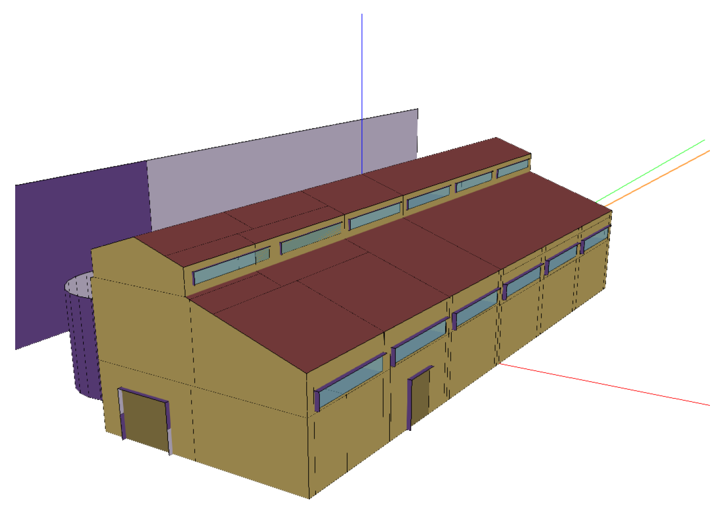
• MixedUse: A building with 13 thermal zones (eight controlled with thermostats) used for residential and office spaces. It is also located in the Attica region of Greece. Both the envelope and the technical systems were calibrated with the corresponding test site data.
• Seminarcenter: This building encapsulates 27 thermal zones, belonging to 22 rooms of which 18 are controlled with thermostats. It is located in the Region of Southern Denmark. Both the envelope and the technical systems were calibrated with the corresponding test site measurements.
• SimpleHouse: This building is a standard single room house with HP and sun heating effects through glazing. Two versions exist, one with a standard radiator (SimpleHouseRad) and the other one with floor heating (SimpleHouseSlab). The first order envelope model is designed based on thermal peak power and minimal outdoor temperature.
• SwissHouse: This building is a large-scale version of the SimpleHouse building with radiators. It has been designed with parameters (thermal peak power, outdoor temperature) from a real house. The heat pump control differs from the SimpleHouse model, see

  Table A6. Inputs and outputs for the models SimpleHouseRad-v0 and SimpleHouseSlab-v0 (1), and SwissHouseRad-v0 (2).

  Variable Name	Description	Bounds	Units	Model
  Inputs
  u	Heat pump normalized power	[0,1]	-	1
  heaSup.f	Heat pump normalized supply flow	[0,1]	-	2
  heaSup.T	Heat pump supply temperature	[293.15,353.15]	K	2
  Outputs
  TOut.T	Outside Temperature	[253.15,343.15]	K	1/2
  temRoo.T	Room Temperature	[263.15,343.15]	K	1/2
  heaPum.P	Heat pump power	[0,30]	kW	1/2
  temRet.T	Heat pump return temperature	[273.15,353.15]	K	1/2
  temSup.T	Heat pump supply temperature	[273.15,353.15]	K	1/2

  .

The calibration methodology used for the models is explained in Section 4.

3. Library Design and Functionalities

3.1. Design Features

Energym is designed to work with different controller types including rule-based controllers (RBC), MPC controllers and RL-based controllers. Hence the building environments and their interface are provided but the controller structure is not prescribed and left free to the user. Moreover, model performance evaluation is not based on fixed rewards (like in Gym) but implemented via KPIs that can be computed by the user after an evaluation run. The main features of the library are outlined below (A full documentation of the library, describing usage and installation, is available at https://bsl546.github.io/energym-pages/ (accessed on 14 April 2021)).

3.1.1. Standardized Evaluation

For each model outlined in Table 1, a physical objective to be reached is predefined. This objective might be, e.g., the minimization of the CO${}_2$ emissions related to the building operation. The controllers also have to satisfy thermal constraints to guarantee occupant comfort. These two quantities—objective and constraints—are tracked with the implemented KPIs; see Section 3.3,

Table 2. Fixed evaluation scenarios for the simulation models.

Model	Simulation Period	Temperature Constraints (°C)	Objective KPI
ApartmentsThermal-v0	January–April	19–24	Grid exchange
ApartmentsGrid-v0	Entire year	19–24	Grid exchange
Apartments2Thermal-v0	January–April	19–24	Grid exchange
Apartments2Grid-v0	Entire year	19–24	Grid exchange
OfficesThermostat-v0	Entire year	19–24	Power demand
MixedUseFanFCU-v0	Entire year	19–24	Power demand
SeminarcenterThermostat-v0	January–May	21–24	CO${}_2$ emissions
SeminarcenterFull-v0	January–May	21–24	CO${}_2$ emissions
SimpleHouseRad-v0	January–April	19–24	Power demand
SimpleHouseSlab-v0	January–April	19–24	Power demand
SwissHouseRad-v0	January–April	19–24	Power demand

. For each building, the evaluation phase with the predefined KPIs is run over a definite period of time and under predefined weather conditions.

3.1.2. Wrappers

Wrappers are implemented to cope with different controller needs. In particular, wrappers are provided to scale inputs and/or outputs between values in a min-max fashion. The scaling can be beneficial for optimization-based controllers like MPC, due to the used model and solver structure. For RL-controllers, an RL-wrapper is provided to change the outputs of the step method and provide exactly the same outputs as in the Gym library, i.e., outputs, reward, done, info. One slight change with respect to Gym, however, is that the reward design is left free to the user and must be specified at wrapper initialization. This design choice was made for users to be free in the reward design phase, the main objective of any controller being to minimize the predefined KPIs. Similarly, for controller speed-up (in particular for MPC), a downsampling wrapper is provided to optimize computation time, making it possible to solve the problem less frequently than what the standard step method would impose.

3.1.3. Forecasting Capabilities

For designing controllers such as MPC, it is important to have descriptions of external disturbances. For this, we provide weather forecasts (including irradiance and temperatures), optionally given by the exact values in the used weather files or by stochastic variations of those. Furthermore, we provide forecasts that are highly relevant for certain models: EV usage schedules for the Apartments and Apartments2 buildings, and electricity mix forecasts for the Seminarcenter. Random seeds to generate the forecasts are fixed in evaluation mode to ensure reproducibility of the results.

3.2. Usage and Code Example

Basic Structure and Usage

After importing Energym, a model can be created by calling the make method and specifying the name of the model and other optional parameters, i.e., the starting day of the simulation, the number of simulated days, the used weather file, and the used KPIs, all of which use default values if not specified upon initialization. The interaction with the model, i.e., passing control inputs and receiving outputs, is done with the step method. Control inputs are Python dictionaries, with the setpoint name as key and input as value (possibly a list with multiple entries for multiple consecutive inputs), e.g., {"Z01_T_Thermostat_sp":[21]} (or {"Z01_T_Thermostat_sp":[21, 22, 21]}). Outputs are also defined as dictionaries using the predefined output names as keys. The main inputs and outputs for each model are given in Appendix B. A full list is available in the online documentation. The Wrapper class is implemented to provide input-output wrapper functionalities. Weather and stochastic disturbances forecasts are available with the get_forecast method.

For the tracking of the KPIs, a KPI object is initialized for each model, it automatically records the necessary data. Calling the method get_kpi returns the evaluation for a specified time interval (by default all the completed steps) as a dictionary. More details on handling the KPIs and the default ones are discussed in Section 3.3.

A simple usage example is given in Appendix A.1.

3.3. Performance Evaluation

A pre-compiled FMU is provided for each building model and can be used with different weather files. This allows the users to train their controllers (i.e., RL agents or models for MPC) with different weather files, while the weather file for final evaluation is fixed. These fixed weather conditions on a predefined period of time ensure comparability of the control performances via the implemented KPIs. The characteristics of these fixed evaluation scenarios are displayed in Table 2. The defined KPIs fall into the categories of thermal comfort (related to temperature constraints) and objective KPI (related to the objective to minimize).

KPI Definition

For the thermal comfort, a range of acceptable temperatures is defined. The tracked KPIs are the average deviation from the target temperatures for each controlled thermal zone and the total number of range violations. Let the desired temperature range be defined by the interval $I=[a,b]$. Then the average deviation $d(T,I)$ for temperature measurements $T=\{t_i:i=1,\cdots ,N\}$ is defined as

$$d(T,I):=\frac{1}{N}\sum _{i=1}^N{\parallel t_i\parallel }_I$$

(1)

where ${\parallel t\parallel }_I=\left\{\begin{array}{c}a-t,\mathrm{if}t<a\hfill \\ 0,\mathrm{if}t\in I\hfill \\ t-b,\mathrm{if}t>b\hfill \end{array}\right.$.

The number of total violations $v(T,I)$ is defined as

$$v(T,I):=\sum _{i=1}^N\delta (t_i,I)$$

(2)

where $\delta (t,I)=\left\{\begin{array}{c}0,\mathrm{if}t\in I\hfill \\ 1,\mathrm{if}t\notin I\hfill \end{array}\right.$.

The average energy exchanged with the grid is tracked for the models based on the Apartments and Apartments2 buildings. Let $E_{prod}=\{e_{prod,i}:i=1,\cdots ,N\}$ be the set of N consecutive measurements of produced energy and $E_{con}=\{e_{con,i}:i=1,\cdots ,N\}$ of consumed energy. Then the average energy exchange $e(E_{prod},E_{con})$ is defined as

$$e(E_{prod},E_{con}):=\frac{1}{N}\sum _{i=1}^N|e_{prod,i}-e_{con,i}|.$$

(3)

In the evaluation scenario, the goal is to minimize this quantity and therefore maximize the self-consumption of produced energy.

The objective for the Offices, MixedUse, SimpleHouse and SwissHouse buildings is to minimize their power consumption. Let the mean power demand for N simulation steps be given by $D=\{d_i:i=1,\cdots ,N\}$. The minimization objective is again given by averaging over the measurements, so the average power demand $p\left(D\right)$ is defined as

$$p\left(D\right):=\frac{1}{N}\sum _{i=1}^N{d}_i.$$

(4)

The environments based on the Seminarcenter building track the CO${}_2$ emissions for the installed gas boiler and the varying electricity mix. A minimization of this emission is the focus of their evaluation scenario. Let the emission values be given by $C=\{c_i:i=1,\cdots ,N\}$. The computed KPI for those measurements is the average emission $g\left(C\right)$ defined as

$$g\left(C\right):=\frac{1}{N}\sum _{i=1}^N{c}_i.$$

(5)

Instead of using predefined KPIs, it is also possible to define custom KPIs. An example of this is given in Appendix A.2.

4. Calibration Methodology

Distinct methodologies (see Table 1) for calibration have been used, depending on whether the entire building or just the technical systems were calibrated with real data sets. After calibration and validation with standard metrics (see e.g., Section 4.1.2), the model responses to control actions were further tested independently by team members to ensure that physical expectations were met (setpoint responses, energy consumption patterns by system activation, etc.).

4.1. Building Calibration

The Offices, MixedUse and Seminarcenter buildings have been calibrated using the three-step methodology presented in [24]. A short overview of the method is explained in the following.

4.1.1. Method

In the first step, data are collected from the test sites at a 15 min sampling rate. Collected features include weather parameters (outside temperature, ground temperature, relative humidity, irradiance, atmospheric pressure, wind speed), indoor climate (room temperatures and relative humidity), as well as technical equipment parameters (water temperature and flow, on/off status) and electric consumption disaggregated by sources. Standard data pre-processing techniques are applied to the collected data to improve their usability, namely: gap reconstruction (via interpolation), removal of sensor malfunction periods, and on/off status reconstruction for technical systems for which this signal was not made directly available.

In a second step, the buildings are modelled and their envelope calibrated using the collected data. It uses free oscillation data, i.e., periods where the HVAC equipment is off to eliminate HVAC interference. As described in depth in [24], envelope calibration is realized through a parametric analysis, a sensitivity analysis and a genetic algorithm simulation (using the NSGA-II genetic algorithm; see [25]) guided by an appropriate objective function (based on normalized root mean square error (NRMSE), determination coefficient, and normalized mean bias error (NMBE)).

In a third step, HVAC and technical equipment are introduced and configured to supply the building demand. A detailed HVAC model is added to the previously calibrated envelope model and simulated in EnergyPlus. Known HVAC equipment parameters are set to technical specification values, different performance curves are determined for each of the components, while unknown parameters are set either based on technical information of similar equipment, or calculated based on test site data. This detailed model undergoes a new calibration process similar to the one used for the envelope, i.e., a parametric/sensitivity analysis followed by a genetic algorithm simulation guided by a new objective function. This calibration is performed until the simulation model uncertainty indices are acceptable within the expected KPIs; see Section 4.1.2.

4.1.2. Model Evaluation

Three metrics were used to assess the quality of building models: the NMBE, the coefficient of variation of the RMSE (CVRMSE) and the coefficient of determination $R^2$; see e.g., [26]. Model acceptance is based on the threshold values recommended by the American Society of Heating, Refrigerating and Air-Conditioning Engineers (ASHRAE) and the International Performance Measurement and Verification Protocol (IPMVP); see e.g., [26].

4.1.3. Example: The MixedUse Building

Calibration of the envelope parameters for the MixedUse building has been performed with free oscillation data as described in Section 4.1.1. The HVAC system of the MixedUse building is made of two independent main technical systems: a Variable Refrigerant Volume Unit (VRV) and an air-to-water HP. The initial performance curves of these two systems have been fitted with linear estimations to reproduce the suppliers’ technical documentation with the performance equations of the corresponding EnergyPlus objects. For the MixedUse VRV system a total of 14 different curves were required, from cooling and heating capacity for low/high outdoor conditions including its boundary curves to piping length correction and defrosting; see Figure A5 and Figure A6 in Appendix C.1.

Key parameters were then estimated in the next step (nominal power, design airflow, design supply temperature, efficiency, ...) via the optimization process with the NSGA-II genetic algorithm in order to find the combination of parameter values that results in the best fit of energy consumption while maintaining the indoor climate of the building. The results for the VRV system are displayed in

Table A7. Results of VRV system calibration for cooling and heating periods, 2019–2020.

Index	ASHRAE	Cooling	Average	Heating	Average
	Thresholds	Energy	Indoor	Energy	Indoor
(Hourly)		Consumption	Temperature	Consumption	Temperature
			(Main Building)		(Main Building)
DATE	—	May–October	May–October	November 2019–	November 2019–
		2019	2019	April 2020	April 2020
NMBE (%)	within $\pm 10\%$	9.49%	0.16%	17.29%	1.12%
CV(RMSE) (%)	$\le 30\%$	27.57%	1.04%	27.57%	2.75%
R2 (%)	$\ge 75\%$	76.17%	95.50%	66.50%	97.39%

and the results for the HP system in

Table A8. Results of HP system calibration for cooling and heating periods, 2019–2020.

Index	ASHRAE	Cooling	TZ-05	HEATING	TZ-05
	Thresholds	Energy	Indoor	Energy	Indoor
(Hourly)		Consumption	Temperature	Consumption	Temperature
			(Atrium)		(Atrium)
DATE	—	July–October	July–October	November 2019–	November 2019–
		2019	2019	April 2020	April 2020
NMBE (%)	within $\pm 10\%$	7.37%	−0.02%	−7.42%	5.31%
CV(RMSE) (%)	≤$30\%$	27.41%	1.27%	27.21%	8.22%
R2 (%)	≥$75\%$	78.89%	94.51%	76.49%	85.26%

in Appendix C.1.

Finally, the evaluation period took place during Summer 2020, between the months of June and August (i.e., on data not used for identification). Results are displayed in

Table 3. Results of Variable Refrigerant Volume (VRV) and Air Handling Unit (AHU) system evaluation for cooling period, June to August 2020.

Index	ASHRAE	Cooling	Average	Cooling	TZ-05
		Enrgy	Indoor	Supply	Indoor
(Hourly)		Consumption	Temperature	Air	Temperature
		(VRV)	(Main Building)	(AHU)	(Atrium)
Date	—	June–August	June–August	May–July	May–July
		2020	2020	2020	2020
NMBE (%)	$\mathrm{within}10\%$	6.40%	0.33%	1.43%	0.42%
CV(RMSE) (%)	≤30%	29.26%	1.16%	3.62%	1.69%
R2 (%)	≥75%	75.23%	92.73%	85.57%	86.98%

. It should be noted that during the evaluation period the HP underwent a series of malfunctions and had to be repaired. This is why evaluation results for the HP are not presented here.

4.2. Heat Pump Calibration

For the Apartments building, heating is covered by means of a centralized water-to-water geothermal HP system that provides hot water for the indoor fan coil units and the Domestic Hot Water (DHW) tanks. This HP model has been calibrated using real data from a test bench facility installed at the IREC laboratory. The method used is based on the work presented in [27] for HP identification and the water-to-water HP model developed in [28]. Equations (6) and (7) from [28] displayed below represent the fitting of the heating thermal power and of the electric power consumed by the HP. The experimental data used to fit the equations have been obtained by operating the HP at full load in heating mode (control of return temperature to the condenser of the HP).

$$\begin{array}{cc}\hfill \frac{Q_h}{Q_{h_{ref}}}& =D1+D2\left[\frac{T_{L_{in}}}{T_{ref}}\right]+D3\left[\frac{T_{S_{in}}}{T_{ref}}\right]+D4\left[\frac{{\dot{V}}_L}{{\dot{V}}_{L_{ref}}}\right]+D5\left[\frac{{\dot{V}}_S}{{\dot{V}}_{S_{ref}}}\right]\hfill \end{array}$$

(6)

$$\begin{array}{cc}\hfill \frac{P_h}{P_{h_{ref}}}& =E_1+E_2\left[\frac{T_{L_{in}}}{T_{ref}}\right]+E3\left[\frac{T_{S_{in}}}{T_{ref}}\right]+E4\left[\frac{{\dot{V}}_L}{{\dot{V}}_{L_{ref}}}\right]+E5\left[\frac{{\dot{V}}_S}{{\dot{V}}_{S_{ref}}}\right]\hfill \end{array}$$

(7)

where:

• $D1$–$D5$, $E1$–$E5$: Fitting coefficients for heating mode
• $T_{ref}=283.15$: Reference temperature, [K]
• $T_{L_{in}}$: Temperature of water entering the load side, [K]
• $T_{S_{in}}$: Temperature of water entering the source side, [K]
• ${\dot{V}}_L$: Load side volumetric flow rate, [m${}^3$/s]
• ${\dot{V}}_{L_{ref}}$: Reference load side volumetric flow rate, [m${}^3$/s]
• ${\dot{V}}_S$: Source side volumetric flow rate, [m${}^3$/s]
• ${\dot{V}}_{S_{ref}}$: Reference source side volumetric flow rate, [m${}^3$/s]
• $P_h$: Power consumption [kW]
• $P_{h_{ref}}=3.89$: Rated heating power consumption [kW]
• $Q_h$: Condenser heating rate [kW]
• $Q_{h_{ref}}=42.49$: Rated condenser heating rate [kW]

A constant volumetric flow rate was used in the experiment as the pump was operating with a constant flow, hence ${\dot{V}}_L={\dot{V}}_{L_{ref}}$ and ${\dot{V}}_S={\dot{V}}_{S_{ref}}$. Coefficients were fitted to the data using ordinary least squares. The $Q_h$ calculation residuals range from 0.01–3.94% of the $Q_h$ value (max. deviation of 1.45 kW for a nominal consumption of 36.8 kW heating power) and are displayed in Figure 1a. The corresponding $R^2$ value for the heating power fitting is 0.985. $P_h$ residuals range from 0.02–4.78% of the electric power consumption value (max. deviation of 0.29 kW for an electrical power consumption of 6.24 kW). The $R^2$ value for the electric power fitting is 0.988. The residuals are depicted in Figure 1b.

4.3. Modelica Models

Modelica models are developed with components from the LBNL Modelica Buildings Library [29]. While one of the strengths of EnergyPlus is the ease at which large and realistic envelope models can be built, Modelica models with large and complex envelopes are harder to design: The strength of Modelica is the realism and flexibility at disposal for modeling and controlling technical systems like HPs, storage tanks, and AHUs. This is the reason why the currently included models come with very simple envelopes, but complex and realistic technical systems, the other case being covered by the EnergyPlus models at disposal. Future Modelica models with more complex envelopes are in preparation and will be integrated to the library. The authors also do not exclude incorporating models using Modelica for the control systems and Energyplus envelopes.

The envelope model used for SimpleHouse and SwissHouse is a simple first order model calibrated with the thermal peak power, minimum outdoor temperatures and the building free oscillation time constant. The indoor temperature is averaged over the house geometry and modeled by a scalar $T\left(t\right)$ obeying Equation (8).

$$C\frac{dT}{dt}\left(t\right)=Q_{\mathrm{flow}}\left(t\right)-G(T\left(t\right)-T_{out}\left(t\right))$$

(8)

Assuming equilibrium at very cold temperatures, the thermal conductance G [W/K] is deduced by setting the left-hand side equal to zero in these conditions. G [W/K] is then inferred to be equal to the ratio of the thermal peak power over the indoor-outdoor temperature difference for the four coldest consecutive days on the last 20 years (see SIA norm CT 2028:2010 [30]). Knowing the thermal conductance G and inferring the time constant $\tau$ of the envelope from the available building data, we derive the heat capacity C [J/K] = $G\tau$.

For SwissHouse models, these G and C correspond to an overall U-value of 0.5 [W/m${}^2$K] and to a heat capacity per surface unit of 0.2 [MJ/m${}^2$K], resulting in a time constant $\tau$ of >4 days, for this type of low energy building with a heat demand of 15 [W/m${}^2$]. For air-to-water HP, the typical seasonal coefficient of performance (COP) is 3, which gives a nominal electric power of 5 [W/m${}^2$].

5. Conclusions and Future Directions

The library Energym presented in this paper aims at providing building models and standardized evaluation scenarios and metrics to develop, test, and benchmark controllers. With diverse equipment configurations calibrated with real measurement data, Energym has been designed to ease the development and deployment of “swiss knife” data-driven controllers for buildings. The used calibration methods and results have been outlined.

Two main axes of research are foreseen for future works: The extension of the library itself and the development of data-driven control methods tested on the library.

For the former, Energym is aimed at growing by gaining new building models. We are currently developing new models (both Energyplus and Modelica models) that will be incorporated into the library in the near future. Moreover, through releasing Energym as open-source, we encourage model contributions from the building simulation community (To add a new model, please contact the authors.) and the authors welcome such efforts.

For the latter, MPC and RL-based control strategies will be extensively tested on many buildings of the library to showcase its benchmarking capabilities. Furthermore, since running models in parallel is possible with Energym, we aim to investigate scenarios with multiple models in a district setting and related control problems. Finally, an additional goal of Energym is to increase engagement within the Machine Learning community, in particular the RL community, to problems related to reducing energy consumption and CO${}_2$ emissions.

References

1. Global Alliance for Buildings and Construction. 2019 Global Status Report for Buildings and Construction: Towards a Zero-Emission, Efficient and Resilient Buildings and Construction Sector; Technical Report, International Energy Agency and the United Nations Environment Programme; Global Alliance for Buildings and Construction: Berlin, Germany, 2019. [Google Scholar]
2. IEA. Tracking Buildings 2020; Technical Report; IEA: Paris, France, 2020; Available online: https://www.iea.org/reports/tracking-buildings-2020 (accessed on 14 April 2021).
3. O’Neill, Z.; Li, Y.; Williams, K. HVAC control loop performance assessment: A critical review (1587-RP). Sci. Technol. Bulit Environ. 2017, 23, 619–636. [Google Scholar] [CrossRef] [Green Version]
4. Behrooz, F.; Mariun, N.; Marhaban, M.; Mohd Radzi, M.; Ramli, A. Review of Control Techniques for HVAC Systems—Nonlinearity Approaches Based on Fuzzy Cognitive Maps. Energies 2018, 11, 495. [Google Scholar] [CrossRef] [Green Version]
5. Mařík, K.; Rojíček, J.; Stluka, P.; Vass, J. Advanced HVAC Control: Theory vs. Reality. IFAC Proc. Vol. 2011, 44, 3108–3113. [Google Scholar] [CrossRef] [Green Version]
6. Oldewurtel, F.; Parisio, A.; Jones, C.N.; Morari, M.; Gyalistras, D.; Gwerder, M.; Stauch, V.; Lehmann, B.; Wirth, K. Energy efficient building climate control using Stochastic Model Predictive Control and weather predictions. In Proceedings of the 2010 American Control Conference, Baltimore, MD, USA, 30 June–2 July 2010; IEEE: Piscataway, NJ, USA, 2010; pp. 5100–5105. [Google Scholar] [CrossRef] [Green Version]
7. Ma, Y.; Borrelli, F.; Hencey, B.; Coffey, B.; Bengea, S.; Haves, P. Model Predictive Control for the Operation of Building Cooling Systems. IEEE Trans. Control. Syst. 2012, 20, 796–803. [Google Scholar] [CrossRef] [Green Version]
8. Moroşan, P.D.; Bourdais, R.; Dumur, D.; Buisson, J. Building temperature regulation using a distributed model predictive control. Energy Build. 2010, 42, 1445–1452. [Google Scholar] [CrossRef]
9. Schubnel, B.; Carrillo, R.; Taddeo, P.; Canal Casals, L.; Salom, J.; Stauffer, Y.; Alet, P.J. State-space models for building control: How deep should you go? J. Build. Perform. Simul. 2020, 13, 707–719. [Google Scholar] [CrossRef]
10. Tanaskovic, M.; Sturzenegger, D.; Smith, R.; Morari, M. Robust Adaptive Model Predictive Building Climate Control. IFAC-PapersOnLine 2017, 50, 1871–1876. [Google Scholar] [CrossRef]
11. Chen, B.; Cai, Z.; Bergés, M. Gnu-RL: A Precocial Reinforcement Learning Solution for Building HVAC Control Using a Differentiable MPC Policy. In Proceedings of the 6th ACM International Conference on Systems for Energy-Efficient Buildings, Cities, and Transportation, BuildSys ’19, New York, NY, USA, 13–14 November 2019; Association for Computing Machinery: New York, NY, USA, 2019; pp. 316–325. [Google Scholar] [CrossRef]
12. Wei, T.; Wang, Y.; Zhu, Q. Deep Reinforcement Learning for Building HVAC Control. In Proceedings of the 54th Annual Design Automation Conference 2017, Austin, TX, USA, 18–22 June 2017. [Google Scholar] [CrossRef]
13. Schubnel, B.; Carrillo, R.E.; Alet, P.J.; Hutter, A. A Hybrid Learning Method for System Identification and Optimal Control. IEEE Trans. Neural Netw. Learn. 2020, 1–15. [Google Scholar] [CrossRef] [PubMed]
14. Drgoňa, J.; Arroyo, J.; Cupeiro Figueroa, I.; Blum, D.; Arendt, K.; Kim, D.; Ollé, E.P.; Oravec, J.; Wetter, M.; Vrabie, D.L.; et al. All you need to know about model predictive control for buildings. Annu. Rev. Control 2020, 50, 190–232. [Google Scholar] [CrossRef]
15. Maddalena, E.T.; Lian, Y.; Jones, C.N. Data-driven methods for building control—A review and promising future directions. Control Eng. Pract. 2020, 95, 104211. [Google Scholar] [CrossRef]
16. Crawley, D.B.; Pedersen, C.O.; Lawrie, L.K.; Winkelmann, F.C. EnergyPlus: Energy Simulation Program. ASHRAE J. 2000, 42, 49–56. [Google Scholar]
17. Mattsson, S.E.; Elmqvist, H. Modelica—An International Effort to Design the Next Generation Modeling Language. IFAC Proc. Vol. 1997, 30, 151–155. [Google Scholar] [CrossRef]
18. Lukianykhin, O.; Bogodorova, T. ModelicaGym: Applying Reinforcement Learning to Modelica Models. In Proceedings of the 9th International Workshop on Equation-Based Object-Oriented Modeling Languages and Tools, EOOLT ’19, Berlin, Germany, 5 November 2019; ACM: New York, NY, USA, 2019; pp. 27–36. [Google Scholar] [CrossRef] [Green Version]
19. Moriyama, T.; De Magistris, G.; Tatsubori, M.; Pham, T.H.; Munawar, A.; Tachibana, R. Reinforcement Learning Testbed for Power-Consumption Optimization. In Methods and Applications for Modeling and Simulation of Complex Systems; Li, L., Hasegawa, K., Tanaka, S., Eds.; Springer: Singapore, 2018; pp. 45–59. [Google Scholar]
20. Blum, D.; Jorissen, F.; Huang, S.; Chen, Y.; Arroyo, J.; Benne, K.; Li, Y.; Gavan, V.; Rivalin, L.; Helsen, L.; et al. Prototyping The BOPTEST Framework for Simulation-Based Testing of Advanced Control Strategies in Buildings. In Proceedings of the 16th International Conference of IBPSA, Rome, Italy, 2–4 September 2019; pp. 2737–2744. [Google Scholar] [CrossRef]
21. Vázquez-Canteli, J.R.; Kämpf, J.; Henze, G.; Nagy, Z. CityLearn v1.0: An OpenAI Gym Environment for Demand Response with Deep Reinforcement Learning. In Proceedings of the 6th ACM International Conference on Systems for Energy-Efficient Buildings, Cities, and Transportation, BuildSys ’19, New York, NY, USA, 13–14 November 2019; Association for Computing Machinery: New York, NY, USA, 2019; pp. 356–357. [Google Scholar] [CrossRef]
22. Brockman, G.; Cheung, V.; Pettersson, L.; Schneider, J.; Schulman, J.; Tang, J.; Zaremba, W. OpenAI Gym; Technical Report; OpenAI: San Francisco, CA, USA, 2016. [Google Scholar]
23. Blochwitz, T.; Otter, M.; Åkesson, J.; Arnold, M.; Clauss, C.; Elmqvist, H.; Friedrich, M.; Junghanns, A.; Mauss, J.; Neumerkel, D.; et al. Functional Mockup Interface 2.0: The Standard for Tool independent Exchange of Simulation Models. In Proceedings of the 9th International Modelica Conference, Munich, Germany, 3–5 September 2012; pp. 173–184. [Google Scholar] [CrossRef] [Green Version]
24. Ruiz, G.R.; Bandera, C.F.; Temes, T.G.A.; Gutierrez, A.S.O. Genetic algorithm for building envelope calibration. Appl. Energy 2016, 168, 691–705. [Google Scholar] [CrossRef]
25. Deb, K.; Pratap, A.; Agarwal, S.; Meyarivan, T. A fast and elitist multiobjective genetic algorithm: NSGA-II. IEEE Trans. Evol. Comput. 2002, 6, 182–197. [Google Scholar] [CrossRef] [Green Version]
26. Ruiz, G.R.; Bandera, C.F. Validation of calibrated energy models: Common errors. Energies 2017, 10, 1587. [Google Scholar] [CrossRef] [Green Version]
27. Fuentes, E.; Salom, J. Validation of black-box performance models for a water-to-water heat pump operating under steady state and dynamic loads. E3S Web. Conf. 2019, 111, 01068. [Google Scholar] [CrossRef] [Green Version]
28. Tang, C.C. Modeling Packaged Heat Pumps in a Quasi-Steady State Energy Simulation Program. Master’s Thesis, Oklahoma State University, Stillwater, OK, USA, 2005. Available online: https://hvac.okstate.edu/sites/default/files/pubs/theses/MS/27-Tang_Thesis_05.pdf (accessed on 14 April 2021).
29. Wetter, M. Modelica Buildings library. J. Build. Perform. Simul. 2014, 7, 253–270. [Google Scholar] [CrossRef]
30. Swiss Society of Engineers and Architects. Klimadaten für Bauphysik, Energie- und Gebäudetechnik, SIA 2028:2010. Available online: http://shop.sia.ch/normenwerk/architekt/sia%202028/f/2010/D/Product (accessed on 14 April 2021).
Figure 1. Residuals from the Heat Pump (HP) calibration.
Applsci 11 03518 g001