Abstract
Determining the uniaxial compressive strength of intact rock is the primary objective of a geomechanical project, and a reliable estimate in the early phases saves time and costs for more sophisticated laboratory tests. The problem is knowing which of the correlations between the resistance to uniaxial compression and point load index are reliable, those that cover one or several types of rock (depending on the type of statistical adjustment). In this work, they were evaluated with respect to limestone and travertine from experimental results, and the statistical models of the scale effect of the point load index were determined, and the uniaxial compressive strength being estimated from correlations reported in literature. The limestone model was ascending (strength increases as diameter increases), while the travertine model was descending (strength decreases as diameter increases), obtaining similar exponents for the scale effect equations modeled from the uniaxial compressive strength and point load index in both cases.
1. Introduction
Determining the compressive strength of a rock mass is one of the main objectives that geomechanical design projects address, because it depends not only on the rock material (intact rock), but also on the discontinuities that separate the intact rock blocks. The main parameter used to represent the strength of the intact rock is the uniaxial compressive strength (σc), and it is determined in the laboratory using cylindrical specimens according to the standards of American Society for Testing and Materials (ASTM) [1,2] and International Society for Rock Mechanics and Rock Engineering (ISRM) [3].
In the same way that it can be determined in the laboratory directly, indirect methods have also been developed to estimate σc for almost types of rock in general, and limestone and travertine in particular, because it can be correlated experimentally with its index properties. In this way, predictive models emerge that experimentally relate σc and porosity [4,5,6,7,8,9], σc and density [7,10,11], and σc and the point load index [3,10,12,13,14,15,16,17,18,19,20,21,22] or the number of rebounds of the Schmidt hammer [10,18,23,24,25], which will be seen throughout this work.
This work emphasizes the effect of geometry of the specimens, due to its importance in the magnitude of the value of σc, since both ASTM [1,2] and ISRM [3] recommend cylindrical specimens with a diameter (d) between 50 and 54 mm—reference value according to the scale effect [26]—and a height/diameter ratio (H/d) of between 2 and 3 [27,28,29].
Both d and H/d are very important in the experimental correlations because these are parameters directly related to the values used in the least squares adjustment and linear regression analysis, so the d of the specimen tested under uniaxial compressive stress will be the reference of the predictive model. Therefore, if the values of σc obtained from specimens of 48 mm diameter are correlated by means of a simple (or multiple) regression analysis with those corresponding to any index property, the predictive model will estimate a value of σc of 48 mm and not 50 mm. Between 48 and 50 mm there is almost no difference, but smaller diameters are also used in research, such as 21 mm [30], for example.
For this reason, González et al. [31] and Saldaña et al. [32] used P wave velocity values (vp), measured in cylindrical specimens of 31 mm diameter, in experimental correlations determined for other diameters, thus estimating an erroneous σc value. This led them to the generation of their own experimental predictive models.
Finally, the objective of this research is to determine the experimental correlation between σc and Is for limestone and travertine, for diameters of 31 mm and 50 mm, from the experimental Is(50) and σc(50) estimated from the literature referring to the correlations between σc and Is. There was a special emphasis on the geometry of the specimen tested for each of the tests, which led to studying the scale effect for both rocks because (most of) the correlations referred to the 50 mm diameter.
1.1. Correlation between Uniaxial Compressive Strength and Point Load Index
The point load index is an indirect way of estimating the σc of rock, and there is a wide range of correlations for this. During the early days of this test, it was determined based on the uncorrected point load index (Is) [12,13], but later the use of the point load index corrected for a diameter of 50 mm (Is(50)) was widespread due to the publication of the scale effect of the point load index by Brook [16], analogous to that of Hoek and Brown [33,34] for the σc from cylindrical specimens of intact rock.
Table 1 shows the different correlations for limestone and travertine, from which the dimensions of the test specimens were extracted to determine σc and the corresponding ones to determine Is or Is(50). The point load tests were mainly carried out with diametrically loaded cylinders (Equations (1)–(5), (10), (15) and (16)), but also with axially and diametrically loaded cylinders (Equation (9)) or with regular blocks (Equations (11)–(13)). Another case is the correlations obtained from the results of other publications, such as that of Brook [16] (Equation (8)), analogous to his method of the resistance index for a minimum area of 500 mm2 (T500) (Equation (7)) or those that do not define the geometry or the type of test (Equations (6) and (14)).

Table 1.
Predictive models of uniaxial compressive strength (MPa) from point load index (MPa).
It can be observed that most correlations are linear and pass through the origin of the coordinates, but both ASTM (Equation (18)) and ISRM (Equation (17)) do not clarify the cutoff point with the horizontal axis: ASTM [22] indicates that, if not there are experimental values of σc, Is multiplied by 23 to estimate the uniaxial compressive strength at a diameter of 50 mm (σc(50)) based on Bieniawski [13], while the ISRM [3] indicates that Is(50) must be multiplied by a value between 20 and 25, and can vary between 16 and 60 for anisotropic rocks.
1.2. Correlation between Uniaxial Compressive Strength and the Number of Rebounds of the Schmidt Hammer
The number of rebounds of the Schmidt hammer is another index property that provides information on rock strength. There are two types of hammer depending on their impact energy, L-type (0.735 Nm) and N-type (2.207 Nm). The L-type being is chosen for laboratory correlations due to its lower impact energy since, in this way, the specimens are not broken before the uniaxial compressive strength test, and thus a simple regression analysis can be carried out, since σc and RL come from the same source.
Likewise, there is a correlation between the readings of both hammers (Equation (19)), proposed by Aydin and Basu [37] and collected by the ISRM [38], whose reliability is very high when the number of rebounds of the L-type hammer (RL) is greater than 30, and the number of rebounds of the hammer N-type (RN) is greater than 40:
On the other hand, the ASTM [39] does not distinguish between types of hammer, nor does it recommend an estimate of σc, while the ISRM [38] indicates the corrections for each hammer as a function of the hammer’s position with respect to the horizontal (due to the effect of gravity) and proposes potential and exponential models to estimate σc.
Table 2 shows the main experimental correlations, where three models are exponential (Equations (20), (21), and (23)) and two linear (Equations (22) and (24)). The exponential equations multiply RL or RN and the specific weight to obtain a better adjustment coefficient (R2), as pointed out by Deere and Miller [10].

Table 2.
Predictive models of simple compressive strength (MPa) from the number of rebounds of the Schmidt hammer.
1.3. Scale Effect
Weibull [40] assumed that every solid contains imperfections or defects (microcracks) that diminish the strength of the material due to rupture taking place “as soon as they [weak places] fall within a volume subjected to the stress”. This means that, for two cylinders of different size (but identical shape), the probability of the failure of the large specimen is greater than that of the small one, because it contains more defects, and the strength of the large sample is less than that of the small one [26]. Equation (25) is the generalized modification by which Weibull [41] introduced the positive constant m for a better statistical fit, where σ1 and σ2 are the strength of the two specimens and V1 and V2 the respective volumes, according to Bieniawski [42].
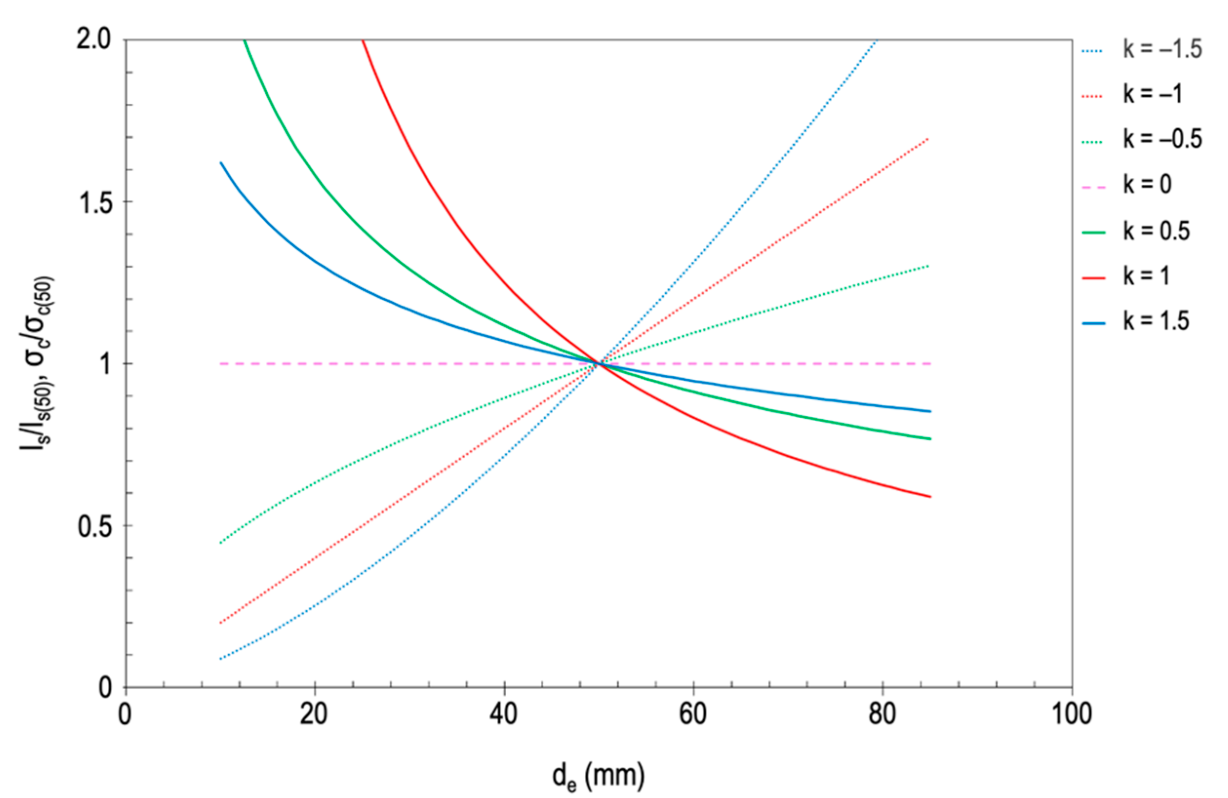
In the case of cylindrical specimens with identical shapes and a constant H/d ratio, the volume can be replaced by d, hence Equations (26) and (27), proposed by Hoek and Brown [33,34] and Brook [16], respectively. It can be seen that the constant 1/m is now called k (Figure 1), so in the case of Hoek and Brown [33,34] the value of k1 is 0.18 and, in that of Brook [16], k2 can be approximated to 0.45. Yoshinaka et al. [43] reported k1 values between 0.1 and 0.3 for hard and homogeneous rocks, while for weathered rocks they are between 0.3 and 0.9. Both correlations refer to the relationship between the strength of the specimen at any diameter (σc, Is) and another at a 50 mm diameter (σc(50), Is(50)).
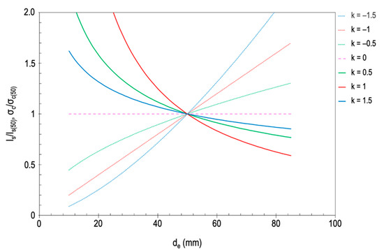
Figure 1.
Effect of the k value (k1 and k2 for Equations (26) and (27), respectively) on the scale effect of rock strength. By definition, k > 0 [41], but negative k values have been added to represent possible ascending models (adapted from Wang et al. [26]).
The models of Hoek and Brown [33,34] and Brook [16] are considered descending, since σc decreases with increasing d. However, the model of Hoek and Brown [33,34] only took into account one sedimentary rock (limestone) of the 10 that it used to generate the experimental model, and also diameters greater than 50 mm. This fact did not go unnoticed by Hawkins [44], who pointed out that the model of Hoek and Brown [33,34] did not adapt to their experimental results obtained from five types of limestone and two of sandstone. To determine σc he tested cylindrical specimens with d values ranging from 12.5 to 150 mm.
Hawkins’s [44] discovery was no longer so much that his results did not fit a descending model with a k1 of approximately 0.18, but that for a diameter less than 40 mm and greater than 60 mm, the results of σc were inferior to those obtained within that interval (mainly 54 mm). In a σc–d graph, this means that for values of diameter less than 40 mm the model is ascending, and the model is descending for values greater than 60 mm. This phenomenon showed that the model of Hoek and Brown [33,34] was not applicable to all types of rock, being able to follow an ascending, descending, or mixed model.
From the energetic point of view, Bazant [45] proposed an alternative descending model to Weibull’s [41], based on Griffith’s [46] theory on the creation and propagation of cracks, which is summarized in two assumptions: (i) when a crack begins to propagate, it is expected that there will be a greater release of energy in the larger specimen under the same stress [47], since it stores more energy than the small one; and (ii) this greater release of energy means that less effort is needed to initiate a crack in larger samples [48]. This model was called the scale effect law (SEL) (Equation (28)):
where σN is the nominal resistance (MPa), B and λ are the dimensionless constants of the material, ft is the strength of a sample with an insignificant size (MPa), d is the diameter of the specimen (mm), and d0 is the maximum diameter of the aggregate (mm).
Nine years later, Bazant [49] proposed a new law to describe ascending models, in which he incorporated fractals (through the fractal dimension df) into the energy required to produce the fracture on concrete, rock, and ceramic. This is the so-called fractal fracture scale effect law (FFSEL) (Equation (29)):
Finally, Masoumi et al. [50] proposed the unified scale-effect law (USEL) (Equation (30)), which is the intersection (di) between the ascending model (FFSEL) and the descending model (SEL), which is applied when there are mixed cases such as limestone and sandstone described by Hawkins [44]. The intersection di is the diameter of the model-change (ascending to descending) in millimeters.
2. Materials and Methods
2.1. Origin of Limestone and Travertine
The limestone belongs to a quarry near Antofagasta (Chile) and dates from the Lower Cretaceous era, between 66 and 100 Ma old. It is a fine limestone rock with a variable CaCO3 content between 78% and 90% [31].
The travertine belongs to a quarry located in Calama, 200 km northeast of Antofagasta (Chile). It belongs to the Chiu-Chiu formation, the youngest within the Calama basin, with an age between 2.5 and 0.5 Ma, from the Upper Pliocene [32].
2.2. Point Load Test
To carry out the test following the suggestions of ASTM [22] and ISRM [3], irregular fragments that meet the specific geometric conditions were selected: the height/width (D/W) ratio of the cross section was between 0.3 and 1. The calculation of the equivalent diameter (de) was carried out according to Equation (31), where D is the distance between the conical tips of the point-load testing machine (height of the cross section) and W the average of the maximum and minimum width of the loaded cross section.
The ISRM [3] suggests determining the σc by multiplying the Is(50) by a factor F that varies between 20 and 25 when the rock does not present anisotropy, as shown in Equation (32), where de is the equivalent diameter (mm), P is the failure load (kN), k2 is the coefficient of the scale factor, and σc is the uniaxial compressive strength (MPa).
This value of k2 is obtained experimentally by a least squares fit in the P−(de)2 graph, discarding all the values that do not belong to the line (but they are not discarded for subsequent calculations of Is(50), just to determine where). However, when there are insufficient experimental values, it is suggested that k2 takes a value of −0.45.
On the other hand, ASTM [22] suggests that to estimate σc when reliable k2 data are not available, it is recommended to take a value from Table 3, based on Bieniawski [13], according to the chosen d (generally 50 mm). When F is 23, it is considered a 50 mm diameter, as presented in Equation (18).

Table 3.
Values of F for different diameters according to American Society for Testing and Materials (ASTM) [22].
2.3. Schmidt Hammer Test
This test is usually performed on the same specimen so that R comes from the same source when performing linear regression analyzes. However, in this case, they were carried out on perfectly parallepipedic plates of more than 70 mm thick (they are more than 54 mm of the cylindrical specimens used in the correlations of Table 2).
The hammer used was N-type and, as indicated by the ISRM [38], 10 readings were made on each surface greater than 1 m2, in a vertical downward position, later correcting its value according to the normalization abacus proposed by Basu and Aydin [51], according to the position of the hammer with respect to the horizontal (and the force of gravity).
2.4. Uniaxial Compressive Strength Test
The tests were carried out using a 300 t CONTROLS servo-controlled press, model 50-C52Z00 + MCC8 50-C8422/M. According to ASTM [1], the loading speed was set to 0.2 MPa·s–1 so that the failure of the specimen occurred between 5 and 10 min after the test started.
The specimen specifications, according to ASTM [2], were an H/d ratio of 2 and the polishing of the basal faces for a better transmission of the force applied by the press.
2.5. Density and Porosity Test
A hydrostatic balance was used to apply the Archimedes thrust principle, collected by the ISRM [3]. The dry mass (mdry) was determined after having the specimens in an oven at 105 °C for 24 h, and the saturated mass (msat) after 48 h immersed in water, while the immersed mass (msub) was obtained by immersing them already saturated to consider the specimen as a solid. The dry density (ρdry), saturated density (ρsat), and effective porosity (neff) were calculated from Equations (33)–(35), respectively:
where mdry is the dry mass (g), msat is the mass of the saturated specimen (g), msub is the mass of the immersed specimen (g), and ρw t is he density of water (g·cm–3).
3. Results and Discussion
The results of d, H, neff, ρdry, ρsat, and σc have already been published by González et al. [31] and Saldaña et al. [32], while those for the point load index (Is) and the N-type Schmidt hammer rebounds (RN) are new. The results of the simple regression analysis for limestone and travertine are presented below, ending with an estimate of the scale effect of σc for both types of rock, in which only the Weibull models are taken into account (Equations (26) and (27)). This decision was taken because only point load index data are available, and there is no information about the change of the trend of the curve for diameters unknown. Finally, from the estimated values of σc(50) and Is(50), the correlations between both properties are made.
3.1. Intact Rock Properties
3.1.1. Limestone
A total of 19 saturated specimens of 31 mm of d and an H/d ratio of 2 were tested, whose results for uniaxial compressive strength, density, and porosity are presented in Table 4. The compressive strength test was performed with saturated specimens, although the results did not differ from those with dry specimens.

Table 4.
Results of the uniaxial compressive strength, density, and porosity tests on limestone.
The average value of ρsat was 2.63 g·cm–3, close to the 2.7 g·cm–3 found by Goodman [52] and within the range between 2.37 and 2.7 g·cm–3, collected by Lama and Vutukuri [53]. The average neff (2.55%) was considered low, according to IAEG [54], and the 68.99 MPa of σc was within the range of 24–290 MPa collected by Zhang [55], and that of Ramírez-Oyanguren and Alejano [56], from 50 to 200 MPa. Regardless of the range, neither the H/d ratio of the specimen nor d is specified in the case of being cylindrical, so these historical data can be collected from different geometries and degrees of weathering.
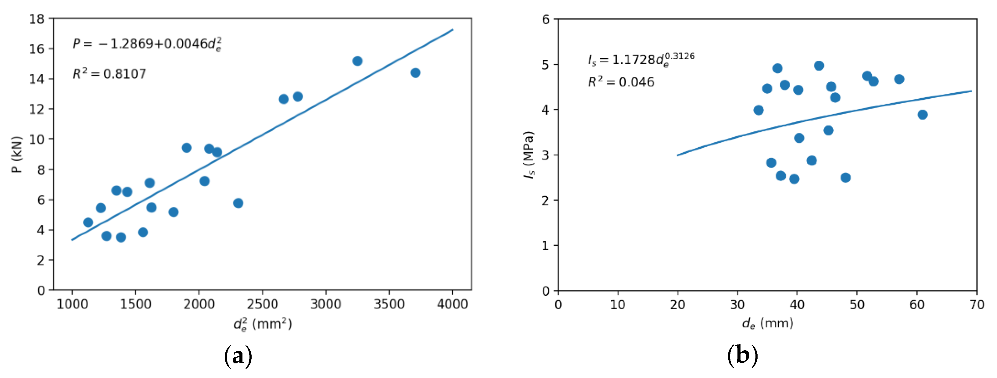
The results of the point load test are presented in Table 5, where the values of Is(50) were determined from Equation (27), with a k2 of −0.3126, obtained experimentally from Figure 2. This suggests that the model is ascending, although it cannot be confirmed whether the decrease in Is begins in the range of 50–60 mm of de, due to a lack of data, as occurs with the limestone of Hawkins [44].

Table 5.
Results of the point load test on limestone.

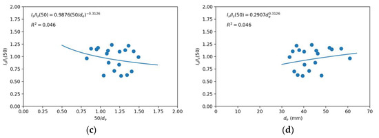
Figure 2.
Scale effect for the point load index of the limestone: (a) quadratic fit of P–de and (b) potential fit of Is–de, to determine the referential value of Is(50); (c) potential fit of Is/Is(50)–50/de and (d) Is/Is(50)–de to determine k2.
Figure 2a shows the P–(de)2 curve, the one designated to determine Is(50), but since data that were part of the same line cannot be discarded [3,22], it was decided to use the Is–de curve (Figure 2b) as a reference, obtaining values of 4.09 and 3.98 MPa, respectively. The average value of these two results (4.03 MPa) was used to determine the curves of the scale effect, Is/Is(50)–50/de (Figure 2c), according to Equation (27), and the most common Is/Is(50)–de (Figure 2d).
3.1.2. Travertine
Analogously to limestone, a total of 29 dry specimens of 31 mm of d and the same H/d ratio of 2 were tested, whose results for compressive strength (with the dry specimen), density, and porosity are presented in Table 6.

Table 6.
Results of the uniaxial compressive strength, density, and porosity tests on travertine.
Table 6 shows an average value for ρdry of 2.43 g·cm–3, within the range between 2.34 and 2.51 g·cm–3 found by authors such as García del Cura et al. [57]. The mean value of neff was 4.05%, within the range of 2.8–34.7% obtained by Soete et al. [58] for “plugs” of 3.81 cm in diameter, which, on the one hand, is very wide due to the irregularity of the distribution of the pores in this type of rock. On the other hand, it is close to the lower limit of the range obtained by García del Cura et al. [57] for 4 × 4 × 4 cm3 cubes, whose experimental range was 5.18–24.99%. The neff value (3.47%) is considered low, according to IAEG [54]. Above 91.72 MPa of σc, it does not fall within a generalized range, as in the case of limestone, since travertine is not a very common rock. In any case, the value of σc(31) is well above the range 30–60 MPa for d between 43 and 54 mm [59,60,61].
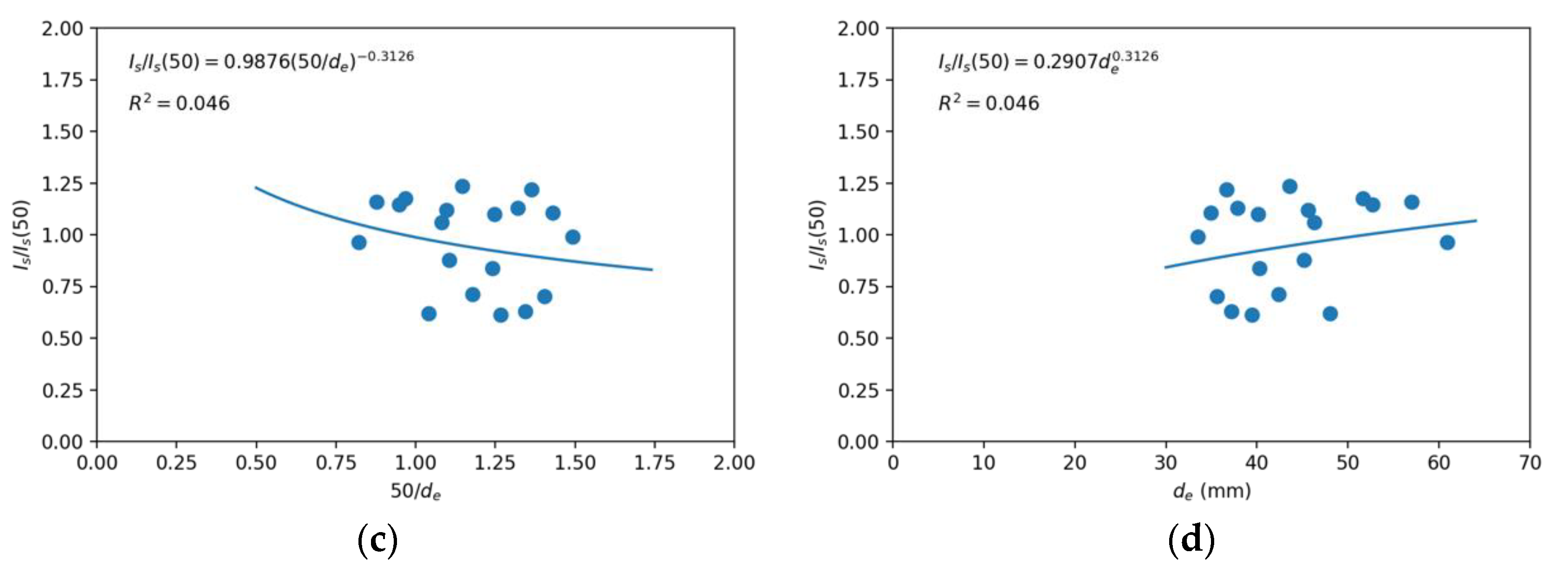
Regarding the point load test, the results are shown in Table 7. The values of Is(50) were determined from Equation (27), with a coefficient k2 of +1.160 obtained experimentally from Figure 3. In this case, it is confirmed that the model is descending, although it is true that the minimum was 44 mm, so it cannot be ruled out that for lower values the model is ascending.

Table 7.
Results of the point load test on travertine.
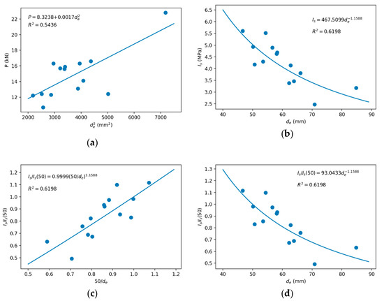
Figure 3.
Scale effect for the point load index of the travertine: (a) quadratic fit of P–de and (b) potential fit of Is–de, to determine the referential value of Is(50); (c) potential fit of Is/Is(50)–50/de and (d) Is/Is(50)–de to determine k2.
Table 8 shows the 30 corrected RN measurements taken on the three plates 7 cm thick and more than 1 m2 in surface area. The corrected results do not fall within any range, since no bibliographic reference has been found in this regard.

Table 8.
Corrected results of the Schmidt hammer test on travertine.
3.2. Correlation between Uniaxial Compressive Strength and Point Load Index without the Scale Effect
For this correlation, Is was used instead of Is(50), because Is(50) depends on the scale effect through k2 (Equation (27)), so it was preferred to carry out a correlation as free as possible from other statistical correlations. Likewise, σc comes from specimens with a d of 31 mm, so it would be appropriate to experimentally correlate σc(31) with Is(31), but the practical application of Is(31) does not reach the level of importance and simplicity of Is and Is(50).
With the linear correlation being y = β0 + β1·x, the intersection with the horizontal axis in this case was 0 (β0 = 0). Finally, when the parameters do not come from the same source, the central limit theorem [62] is applied to the least squares fit, as is the case with σc(31) and Is.
3.2.1. Limestone
To correlate σc(31) with Is, 10 data points for each variable were randomly matched (without repetition) and a linear least squares adjustment was performed.
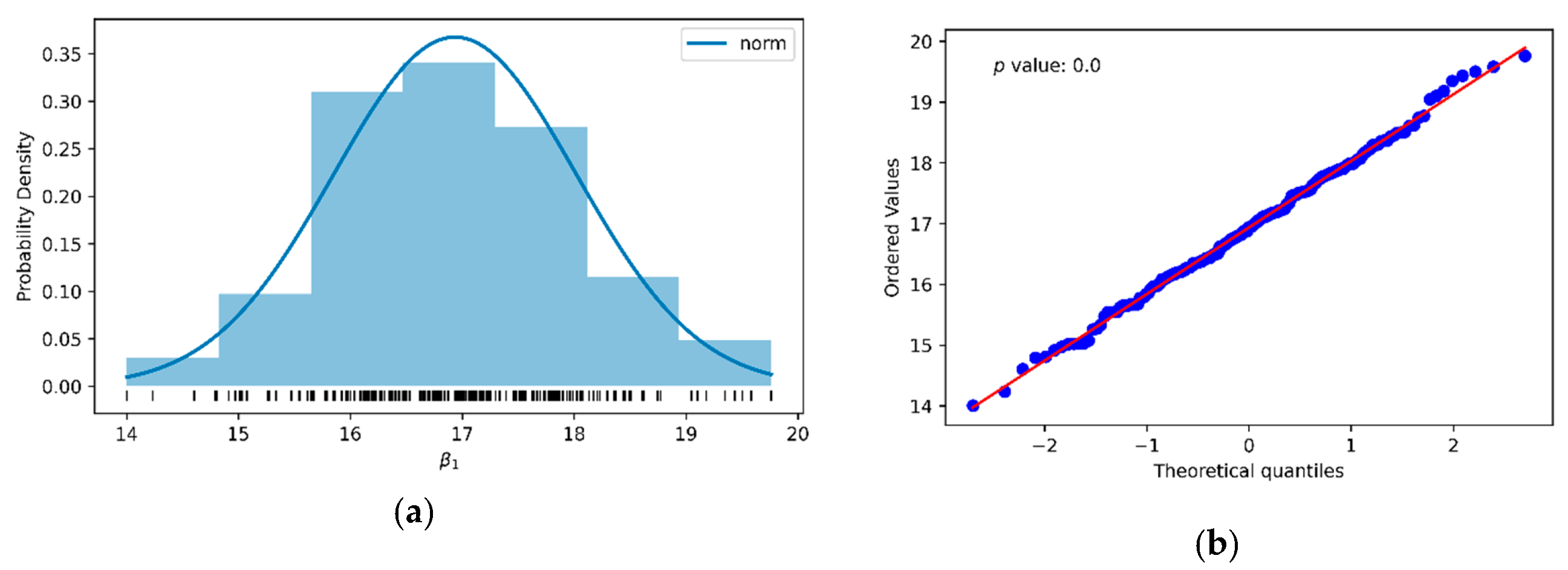
Taking the corresponding values from Table 4 and Table 5 and carrying out 200 random samplings, the histogram in Figure 4a was obtained, which tended to follow a normal distribution with a mean value of β1 of approximately 17 (Equation (36)). The descriptive statistics of the sampling are presented in Table 9, while the normality graph that verified that the data of the β1 statistic were normally distributed is presented in Figure 4b.
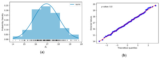
Figure 4.
Histogram with distribution curve (a) and normal probability plot (b) of slope (β1) between σc and Is of the limestone, from the least squares fit of 10 pairs of data points selected from 200 random samples.

Table 9.
Results of the normal distribution of the linear fit for the σc and Is pairs of the limestone.
The relative error between σc(31) from direct and indirect methods was 3.7%. Furthermore, ASTM [22] suggests that β1 = 19 to estimate σc(31) from Is, and the error was −7.6%.
3.2.2. Travertine
As in the previous case, the sampling process was replicated from the data in Table 3 and Table 4, obtaining the data distribution shown in the histogram in Figure 5a, with a mean of β1 of approximately 21 (Equation (37)). The descriptive statistics of the sampling are presented in Table 10, while the normal probability graph shown in Figure 5b corroborated the normality of said statistic (β1).

Figure 5.
Histogram with distribution curve (a) and normal probability plot (b) of slope (β1) between σc and Is of the travertine, from the least squares fit of 10 pairs of data points selected from 200 random samples.

Table 10.
Results of the normal distribution of the linear fit for the σc and Is pairs of the travertine.
Finally, Equation (37) reported a relative error of 12.5%, 91.72 MPa being the experimental σc(31); if 19 [22] is used instead of 21, the error decreases to 3.3%.
3.3. Scale Effect
3.3.1. Limestone
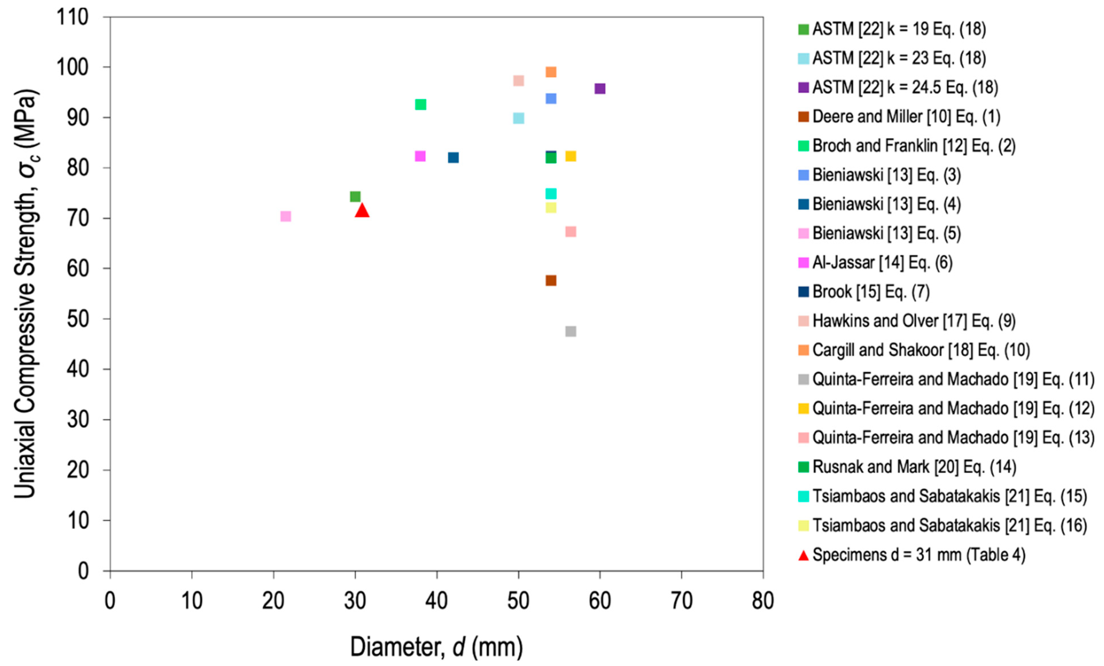
Based on the correlations presented in Table 1 regarding the point load index and σc, the scale effect curve σc–d was estimated for the limestone. The results of σc from all correlations are shown in Figure 6 as colored squares, while the experimental σc(31) is represented by a red triangle. It can be clearly observed that the estimated values of σc generate an ascending model, like in Figure 2d (k2 = −0.3126). Likewise, values that were outside the trend for d less than 50 mm were discarded, since in Figure 2d there are up to 60.9 mm included in the ascending model.
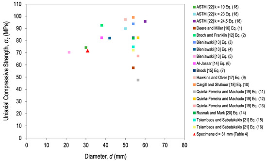
Figure 6.
Estimation of σc from the correlations with Is, Is(50), and Is(50) of Table 1 for limestone.
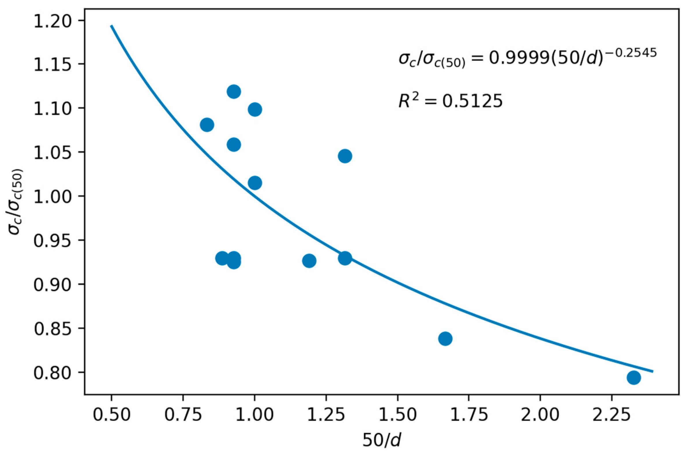
After discarding the lowest values of d in the range of 54–57 mm (Equations (1), (11), (13), (15) and (16)), we had Figure 7, whose adjustment by least squares gives the k1 changed sign. Since k1 is known, it allowed us to calculate the σc(50) of the scale effect corresponding to Equation (27). The values of k1 and σc(50) were −0.2545 and 88.52 MPa, respectively.
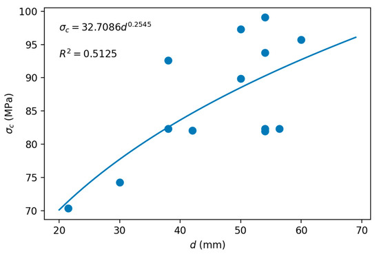
Figure 7.
Least squares adjustment to estimate the σc(50) of the scale effect of the limestone.
Based on the above, the scale effect curve is represented in Figure 8 and the ascending model is given by the following equation:
where the value of k1 (−0.2545) does not correspond to the 0.18 proposed by Hoek and Brown [33,34], neither in sign nor in magnitude, since, as already indicated, the model of this curve was ascending (Figure 7) and not descending.
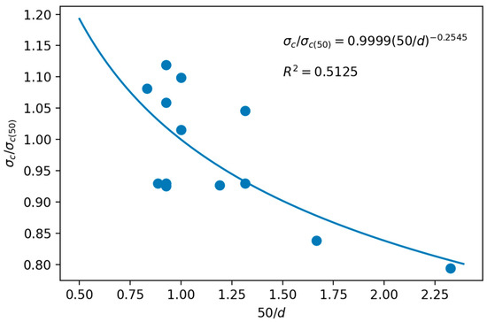
Figure 8.
Scale effect curve from the estimated σc of the limestone.
Another issue is that the value of k1 did not correspond to that of k2 (−0.3126) obtained in the point load test. In this sense, neither Brook [16] nor Wang et al. [26] indicates that the two coefficients must be equal, but σc(50) was estimated by multiplying Is or Is(50) by a constant, so the exponent would not be modified. This suggests that, for the ascending model (Figure 7), the experimental k1 value would be in a range close to the values of –0.3126 and −0.2545.
3.3.2. Travertine
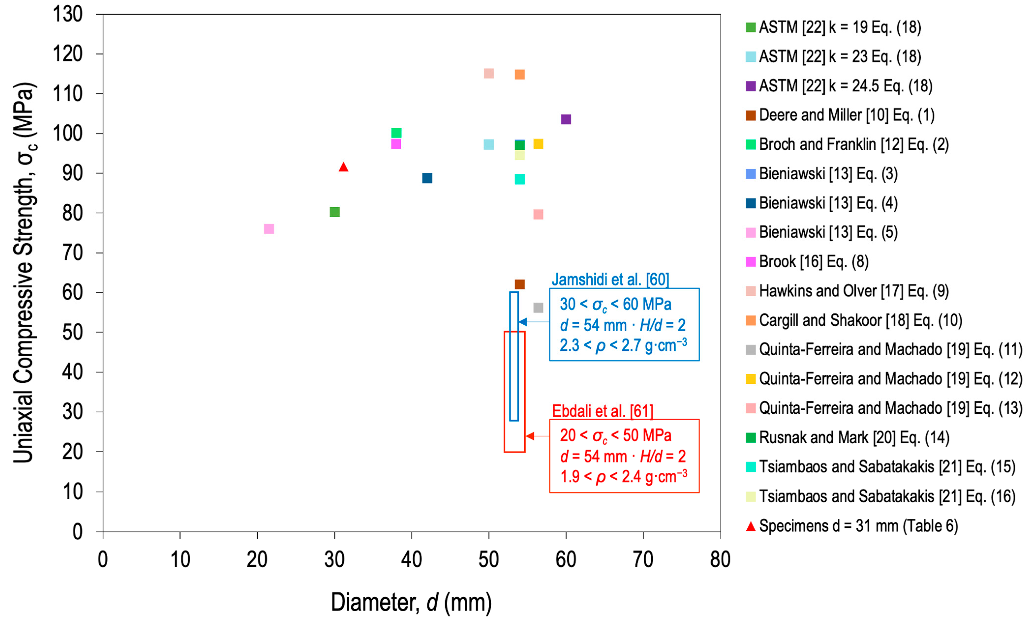
As with the limestone, the composition of travertine is calcium carbonate and, despite the fact that the structure is not the same (mainly due to the distribution of pores and, secondly, to the mineralogical composition being calcite and aragonite), the correlations presented in Table 1 were applied. The results obtained are plotted in Figure 9, in which it can be seen that the main trend of the curve was an ascendent model again, but according to the scale effect of the point load index (Figure 3d), the model should be descending.

Figure 9.
Estimation of σc from the correlations with Is, Is(50), and Is(50) of Table 1 for travertine.
In accordance with the above, Figure 9 shows the area of the results of two investigations in which only travertine was used, those of Jamshidi et al. [60] and Ebdali et al. [61]. In them, σc intervals of 30–60 and 20–50 MPa were recorded, respectively, for a d of 54 mm in both cases. Despite the fact that the model must be descending, according to the experimental results of σc from the point load test, added to the results of Jamshidi et al. [60] and Ebdali et al. [61], these results support the theory of the descending model and not the ascending one. It has to be taken into account that limestone appeared in all the correlations but not for travertine.
In this sense, the curve of the scale effect of travertine (Figure 3d) began with a de of 46.7 mm, so it could not be ruled out with certainty that for lower values the model was ascending and it turned into a mixed (ascending-and-descending) model. Based on this, two curves would be estimated, but due to a lack of data and the dispersion of the existing ones, it was decided that it was too complex (due to uncertainty) and the ascending model would be estimated directly.
To try to shed more light on the trend of the curve, Figure 10 shows the results of σc estimated from the correlations with RL and RN in Table 5. The plotted points (colored squares) did not provide a clear trend (ascending or descending) if the experimental σc(31) (red triangle) was taken into account as the reference value (91.72 MPa from Table 4). However, if it is supposed that the model must be descending, Equations (20) and (24)—proposed by Deere and Miller [10] and Wang and Wan [25], respectively—would provide reliability to the estimated curve of the scale effect.
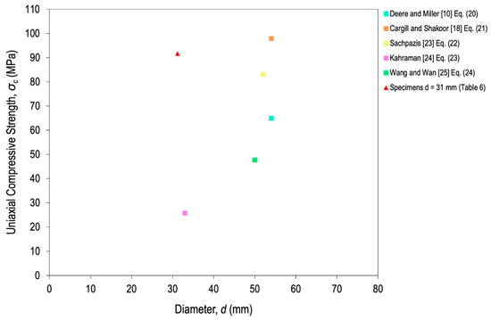
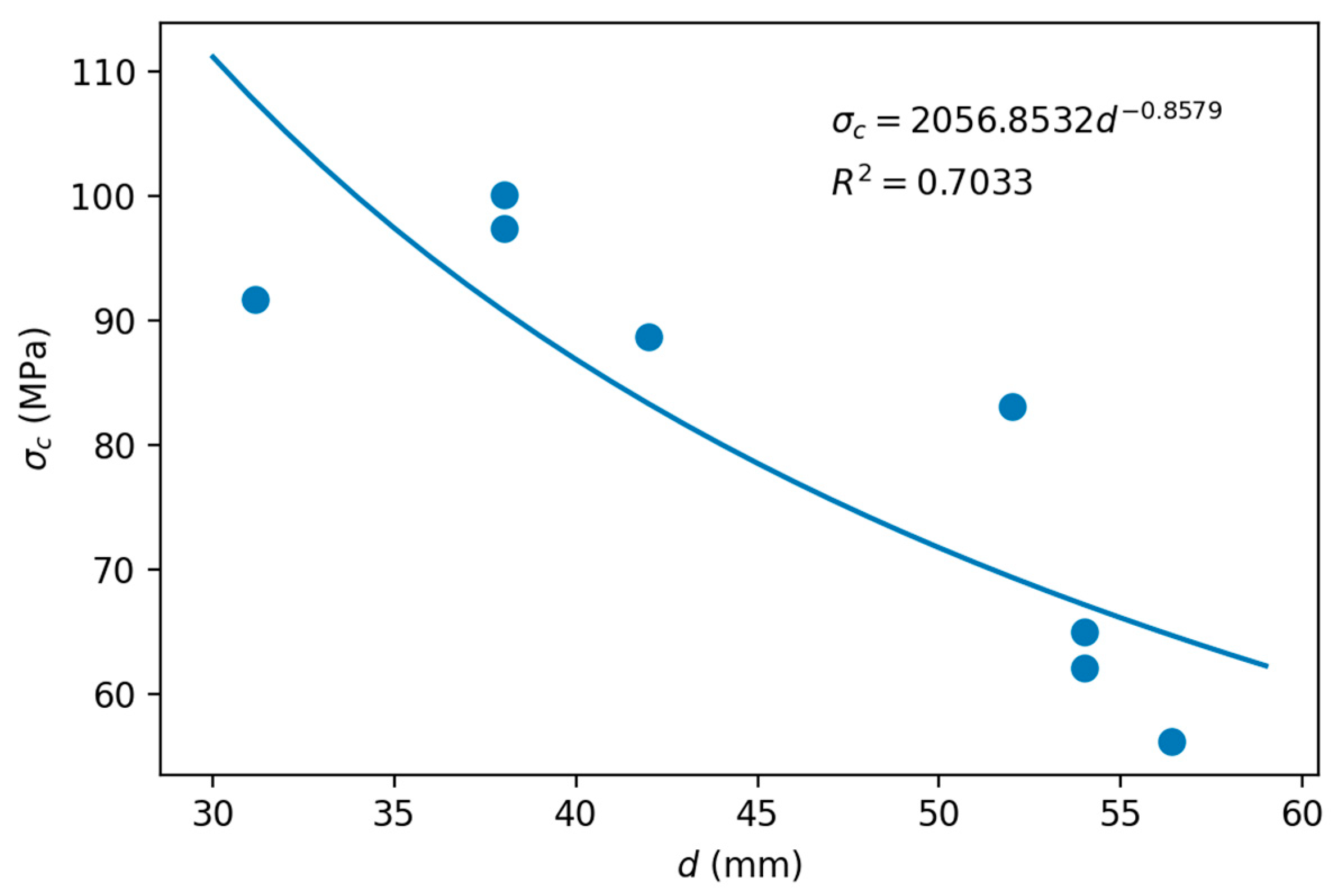
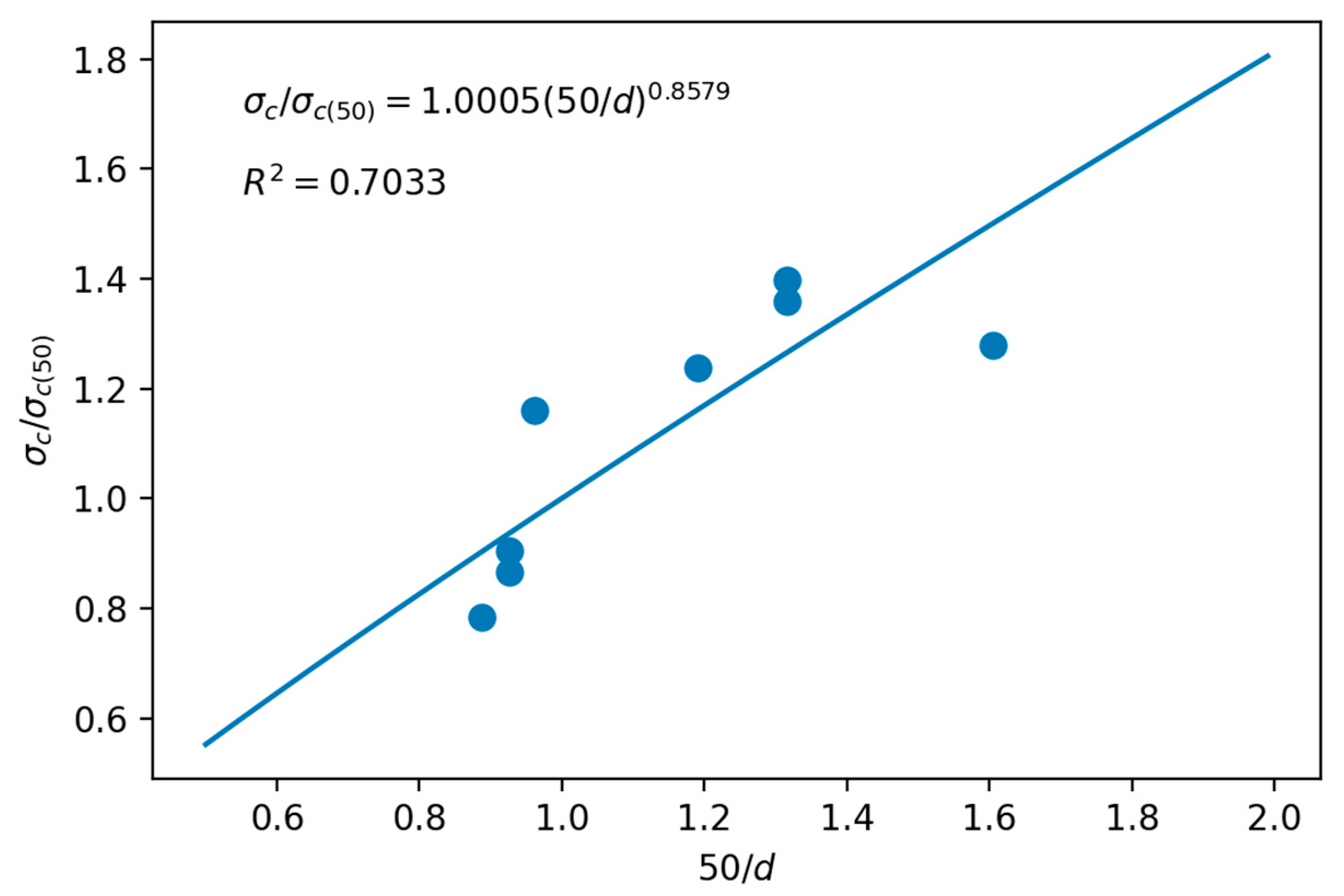
In Figure 11, all the pairs of points from Figure 9 and Figure 10 were plotted, discarding those that are outside of the downward trend. The discarded values corresponded to the correlations for the highest values of d, and are in the range of 54–60 mm. Therefore, the estimates of Equations (1), (2), (4), (6), (11), (19) and (21) were used, together with the σc(31) value (91.72 MPa). After discarding values as necessary, a potential least squares adjustment was carried out, which yielded values of k1 and σc(50) of +0.858 and 71.70 MPa, respectively.
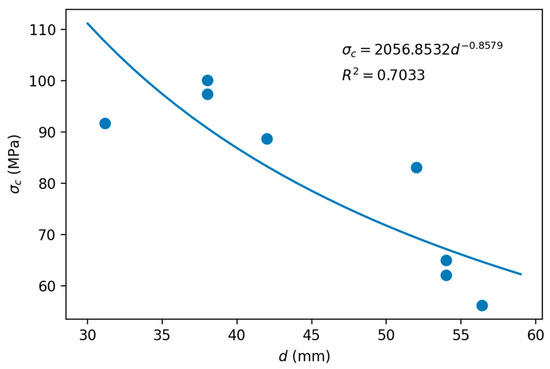
Figure 11.
Least squares adjustment to estimate the σc(50) of the travertine scale effect.
Finally, the scale effect curve, represented in Figure 12, is given by the following equation:
where the value of k1 (0.8579) differs from the 0.18 proposed by Hoek and Brown [33,34], and from the value of k2 of +1.160 obtained in the point load test. As discussed in the case of limestone, Brook [16] and Wang et al. [26] do not indicate that the two coefficients should be equal, but it is assumed that the two coefficients should be similar. To support this assertion, it could be thought that the experimental k1 value would have more weight due to its relatively low dispersion (R2 = 0.6198), but in the absence of more data the experimental interval was between 0.8579 and 1.160.

Figure 12.
Scale effect curve for the σc of travertine.
3.4. Correlation between Uniaxial Compressive Strength and Point Load Index
3.4.1. Limestone
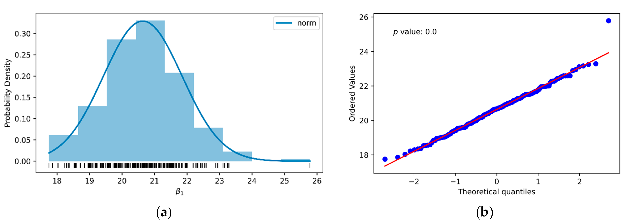
Finally, and because it is one of the reference equations in the point load test suggested by ISRM [3], the correlation between σc(50) and Is(50) is determined from Equations (26) and (27) with k1 of −0.2545 and k2 of −0.3126. Using the results of Table 4 and Table 5 to determine both parameters, we proceeded to randomly combine 10 data pairs from each one of them to carry out a linear adjustment by ordinary least squares [62]. After 200 repetitions (Figure 13), the central limit theorem (Table 11) was applied to determine Equation (37). As can be seen, β1 (20.6) was just above the lower limit of the 20–25 range suggested by the ISRM (Equation (17)), generating an error of −5.2 MPa (−6.8%) regarding Equation (8) by Brook [16], one of the most frequently used methods to estimate σc(50) from Is(50).
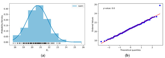
Figure 13.
Histogram (a) and normal distribution graph (b) of the slope β1 of the linear fit by ordinary least squares of 10 data pairs, of σc(50) and Is(50)) of the limestone, randomly selected from 200 random samples.

Table 11.
Results of the normal distribution of the linear fit for the σc and Is(50) pairs of the limestone.
3.4.2. Travertine
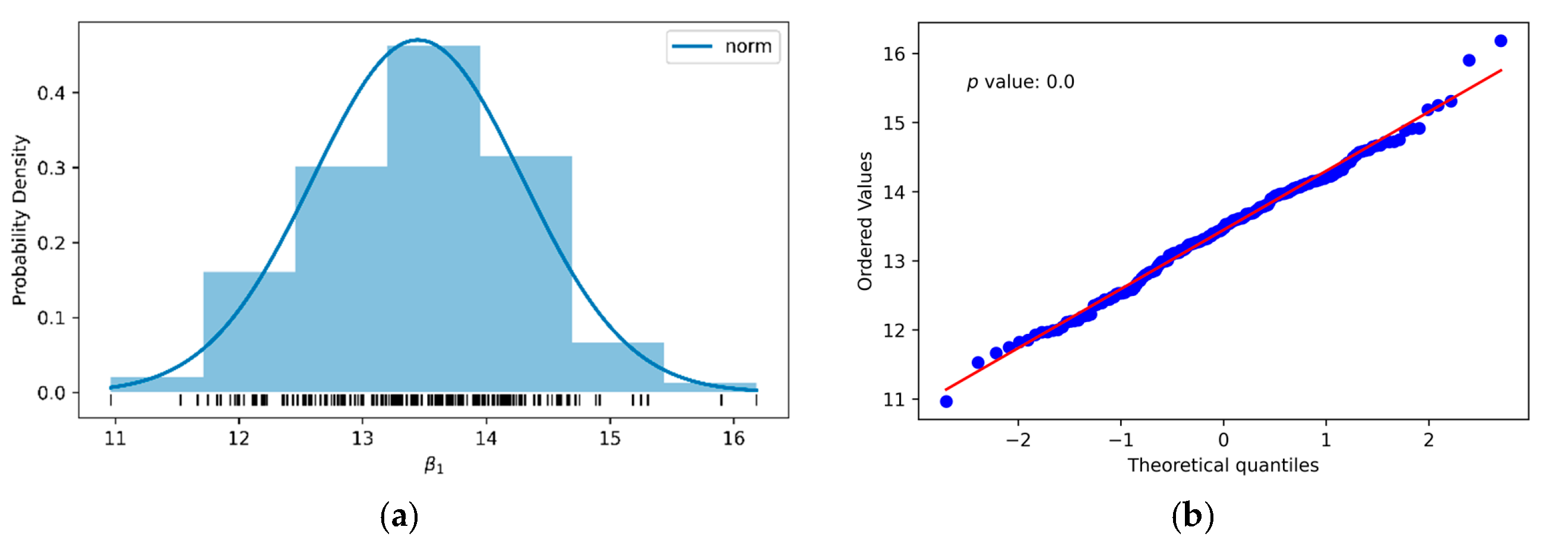
Finally, as with limestone, the travertine correlation between σc(50) and Is(50) was determined due to its impact on the point load test, since the ISRM [3] indicates that β1 was between 20 and 25 for rocks without apparent anisotropy. Then, from Equations (26) and (27), with k1 of +0.858 and k2 of +1.160 and the results of Table 6 and Table 7, we proceeded to combine 10 pairs of random data from the two variables and to perform the linear least squares fit. After 200 repetitions (Figure 14) and applying the central limit theorem (Table 12), Equation (41) was determined. As can be seen in Table 12, β1 (13, 4) was less than 20, the lower range suggested by the ISRM (Equation (17)), with the error with respect to Equation (8) of Brook [16] being −38.1 MPa (−64.2%).
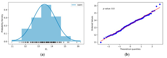
Figure 14.
Histogram (a) and normal distribution graph (b) of the slope β1 of the linear fit by ordinary least squares of 10 data pairs, of σc(50) and Is(50)) of the travertine, randomly selected from 200 random samples.

Table 12.
Results of the normal distribution of the linear fit for the σc and Is pairs of the travertine.
4. Conclusions
After having carried out the tests of uniaxial compressive strength for 31-mm specimens, and point load with irregular samples of saturated limestone and dry travertine, the corresponding values of Is and Is(50) were obtained to generate the scale effect models and correlate these parameters with σc(31) and σc(50), respectively.
For the correlations between σc(31) and Is, factors (β1) of 17 and 21 were obtained for limestone and travertine, respectively, close to the 19 proposed by Bieniawski [13] for 30 mm (Table 3). The associated errors for both rocks are less than 3 MPa (3.5%) on average, which makes it reliable to estimate the σc(31).
In the case of limestone, the scale effect turned out to have an ascending model (greater resistance at a larger diameter); however, due to the range of the diameter (33.5–66.9 mm), it was not possible to determine whether around 67 mm the model could change to a descending model. This uncertainty is based on the σc results obtained by Hawkins [44] for limestone (ascending-and-descending model), and on the scale effect graph plotted from the estimated values of bibliographic σc (Figure 6), which may change the trend to a descending model over 54 mm of diameter. Noting the dispersion of the results of Is (R2 = 0.046), it was decided to consider only the ascending model, obtaining coefficients k1 and k2 of −0.2545 and −0.3126, respectively. The difference between both coefficients (0.06) generated a margin of error of 19% with respect to k2, the only experimental value used as a reference.
Regarding travertine, the experimental results of Is determined a descending model for the scale effect, with a much lower dispersion than in the case of limestone (R2 = 0.6198) at a range of 46.7–84.8 mm for the diameter. On the other hand, the trend of the curve of the scale effect from the bibliographic estimates of σc (Figure 9) was clearly upward. This reason was attributed to the fact that the bibliographic correlations were directly related to limestone and not to travertine, since, despite being practically 100% CaCO3, the crystalline structure was not the same (calcite versus calcite and aragonite), nor was the distribution of internal pores. Likewise, the test with the Schmidt hammer was carried out to estimate more values of σc and help with the downward trend, with Equations (20) and (24)—proposed by Deere and Miller [10] and Wang and Wan [25], respectively—that were close to the values published by Jamshidi et al. [60] and Ebdali et al. [61] for 54 mm, around 40 MPa.
Although a descending model was considered in its entirety, it could not be ruled out that, for values of diameters lower than 31 mm (the experimental reference value in Figure 9: σc(31)), the model was descending, having a mixed (ascending-and-descending) model with a di around 31 mm. For the descending model, which included the estimates of σc (from Is, Is(50), and RN) that favored this trend, coefficients k1 and k2 of +0.858 and +1.160, respectively, were obtained whose difference of 0.30 generates an error of 25.9% with respect to k2, the only experimental value.
Finally, σc(50) and Is(50) were correlated for limestone and travertine, resulting in a factor (β1) of 20.6 for the former, within the range of 20–25 suggested by the ISRM [3] for isotropic rocks, while for travertine, it was 13.4, below the lower limit. If it is taken into account that the value of β1 generally used is 22 [16], it is only useful for limestone, since the average absolute error of −5 MPa (−6.8%) is acceptable, but not the −38.1 MPa (−64.2%) of travertine.
Author Contributions
Investigation and formal analysis, S.C.; conceptualization, investigation, formal analysis and writing—original draft preparation, J.G.; data curation, and validation, M.S.; writing—review and editing, I.P.-R.; supervision, M.A.G. and N.T. All authors have read and agreed to the published version of the manuscript.
Funding
This research received no external funding.
Institutional Review Board Statement
Not applicable
Informed Consent Statement
Not applicable
Acknowledgments
The authors want to acknowledge Izabott Erazo, Carlos Ampuero, Omar González, and Raúl Pérez for helping to perform the laboratory tests.
Conflicts of Interest
The authors declare no conflict of interest.
References
- ASTM D7012-14. Standard Test Method for Compressive Strength and Elastic Moduli of Intact Rock Core Specimens under Varying States of Stress and Temperatures; American Society for Testing and Materials: West Conshohocken, PA, USA, 2017; Available online: http://www.informationweek.com/news/201202317 (accessed on 2 April 2020).
- ASTM D4543-19. Standard Test Methods for Preparing Rock Core as Cylindrical Test Specimens and Verifying Conformance to Dimensional and Shape Tole-rances; American Society for Testing and Materials: West Conshohocken, PA, USA, 2019; Available online: http://www.informationweek.com/news/201202317 (accessed on 2 April 2020).
- ISRM. The Complete ISRM Suggested Methods for Rock Characterization, Testing and Monitoring: 1974–2006; ISRM Turkish National Group: Ankara, Turkey, 2007. [Google Scholar]
- Tugrul, A.; Zarif, H. Correlation of mineralogical and textural characteristics with engineering properties of selected granitic rocks from Turkey. Eng. Geol. 1999, 51, 303–317. [Google Scholar] [CrossRef]
- Kiliç, A.; Teymen, A. Determination of mechanical properties of rocks using simple methods. Bull. Eng. Geol. Environ. 2008, 67, 237–244. [Google Scholar] [CrossRef]
- Nabaei, M.; Shahbazi, K.; Shadravan, A.; Azad, I. Uncertainty Analysis in Unconfined Rock Compressive Strength Prediction. In Proceedings of the SPE Deep Gas Conference and Exhibition, Manama, Bahrein, 24–26 January 2010. SPE-131719-MS. [Google Scholar] [CrossRef]
- Török, Á.; Vásárhelyi, B. The influence of fabric and water content on selected rock mechanical parameters of travertine, examples from Hungary. Eng. Geol. 2010, 115, 237–245. [Google Scholar] [CrossRef]
- Rabbani, E.; Sharif, F.; Koolivand Salooki, M.; Moradzadeh, A. Application of neural network technique for prediction of uniaxial compressive strength using reservoir formation properties. Int. J. Rock Mech. Min. Sci. 2012, 56, 100–111. [Google Scholar] [CrossRef]
- Çelik, S.B. Prediction of uniaxial compressive strength of carbonate rocks from nondestructive tests using multivariate regression and LS-SVM methods. Arab. J. Geosci. 2019, 12, 193. [Google Scholar] [CrossRef]
- Deere, D.; Miller, R. Engineering Classification and Index Properties for Intact Rock; Technical Report No. AFWL-TR-65-116; Air Force Weapons Laboratory/Kirtland Air Base: Albuquerque, NM, USA, 1966. [Google Scholar]
- Vásárhelyi, B. Statistical Analysis of the Influence of Water Content on the Strength of the Mioecene Limestone. Rock Mech. Rock Eng. 2005, 38, 69–76. [Google Scholar] [CrossRef]
- Broch, E.; Franklin, J.A. The point load test. Int. J. Rock Mech. Min. Sci. Geomech. Abstr. 1972, 9, 669–697. [Google Scholar] [CrossRef]
- Bieniawski, Z.T. The point-load test in geotechnical practice. Eng. Geol. 1975, 9, 1–11. [Google Scholar] [CrossRef]
- Al-Jassar, S.H.; Hawkins, A.B. Geotechnical Properties of the Carboniferous Limestone of the Bristol Area the Influence of Petrography and Cheistry. In Proceedings of the 4th ISRM Congress, Montreux, Switzerland, 2–8 September 1979; pp. 1–14. [Google Scholar]
- Brook, N. Size correction for point load testing. Int. J. Rock Mech. Min. Sci. Geomech. Abstr. 1980, 17, 231–235. [Google Scholar] [CrossRef]
- Brook, N. The equivalent core diameter method of size and shape correction in point load testing. Int. J. Rock. Mech. Min. Sci. Geomech. Abstr. 1985, 22, 61–70. [Google Scholar] [CrossRef]
- Hawkins, A.B.; Olver, J.A.G. Point load tests: Correlation factors and contractual use. An example from the Corallian at Weymouth. Geol. Soc. Eng. Geol. Special Publ. 1986, 2, 269–271. [Google Scholar] [CrossRef]
- Cargill, J.S.; Shakoor, A. Evaluation of empirical methods for measuring the uniaxial compressive strength of rock. Int. J. Rock Mech. Min. Sci. Geomech. Abstr. 1990, 27, 495–503. [Google Scholar] [CrossRef]
- Quinta-Ferreira, M.O.; Machado, A.P.G. Assessing Limestone Strength with the Point Load Test. In Scale Effects in Rock Masses 93, Proceedings of the 2nd International Scale Effects in Rock Masses, Lisbon, Portugal, 25 June 1993; Pinto da Cunha, A., Ed.; CRC Press: Boca Raton, FL, USA, 1993. [Google Scholar]
- Rusnak, J.; Mark, C. Using the point load test to determine the uniaxial compressive strength of coal measure rock. In Proceedings of the 19th International Conference on Ground Control in Mining, Morgantown, WV, USA, 8–10 August 2000; Peng, S.S., Mark, C., Eds.; West Virginia University: Morgantown, WV, USA, 2000; pp. 362–371. [Google Scholar]
- Tsiambaos, G.; Sabatakakis, N. Considerations on strength of intact sedimentary rocks. Eng. Geol. 2004, 72, 261–263. [Google Scholar] [CrossRef]
- ASTM D5731-16. Standard Test Method for Determination of the Point Load Strength Index of Rock and Application to Rock Strength Classifications; American Society for Testing and Materials: West Conshohocken, PA, USA, 2016. [Google Scholar]
- Sachpazis, C. Correlating Schmidt hardness with compressive strength and Young’s modulus of carbonate rocks. Bull. Int. Assoc. Eng. Geol. 1990, 42, 75–83. [Google Scholar] [CrossRef]
- Kahraman, S. Evaluation of simple methods for assessing the uniaxial compressive strength of rock. Int. J. Rock Mech. Min. Sci. 2001, 38, 981–994. [Google Scholar] [CrossRef]
- Wang, M.; Wan, W. A new empirical formula for evaluating uniaxial compressive strength using the Schmidt hammer test. Int. J. Rock. Mech. Min. Sci. 2019, 123, 104094. [Google Scholar] [CrossRef]
- Wang, S.; Masoumi, H.; Oh, J.; Zhang, S. Scale-Size and Structural Effects of Rock Materials; Woodhead Publishing: London, UK, 2020. [Google Scholar]
- Mogi, K. Some precise measurements of fracture strength of rocks under uniform compressive stress. Rock Mech. Eng. Geol. 1966, 4, 41–55. [Google Scholar]
- Mogi, K. Experimental Rock Mechanics; Taylor & Francis: London, UK, 2007. [Google Scholar]
- John, M. The Influence of Length to Diameter Ratio on Rock Properties in Uniaxial Compression; A Contribution to Standardization in Rock Mechanics Testing; Report South African CSIR No ME1083/5; Council for Scientific and Industrial Research: Pretoria, South Africa, 1972; Available online: http://www.informationweek.com/news/201202317 (accessed on 2 April 2020).
- Fener, M. The Effect of Rock Sample Dimension on the P-Wave Velocity. J. Nondestr. Eval. 2011, 30, 99–105. [Google Scholar] [CrossRef]
- González, J.; Saldaña, M.; Arzúa, J. Analytical Model for Predicting the UCS from P-Wave Velocity, Density, and Porosity on Saturated Limestone. Appl. Sci. 2019, 9, 5265. [Google Scholar] [CrossRef]
- Saldaña, M.; González, J.; Pérez-Rey, I.; Jeldres, M.; Toro, N. Applying Statistical Analysis and Machine Learning for Modeling the UCS from P-Wave Velocity, Density and Porosity on Dry Travertine. Appl. Sci. 2020, 10, 4565. [Google Scholar] [CrossRef]
- Hoek, E.; Brown, E.T. Underground Excavations in Rock; Institution of Mining and Metallurgy: London, UK, 1980. [Google Scholar]
- Hoek, E.; Brown, E.T. Empirical Strength Criterion for Rock Masses. J. Geotech. Eng. Div. 1980, 106, 1013–1035. [Google Scholar] [CrossRef]
- D’Andrea, D.V.; Fisher, R.L.; Fogelson, D.E. Prediction of Compressive Strength of Rock from Other Rock Properties; USBM RI 6702; US Department of the Interior, Bureau of Mines: Washington, DC, USA, 1965.
- Deere, D.U. Geological considerations. In Rock Mechanics in Engineering Practice; Stagg, K.G., Zienkiewicz, D.C., Eds.; Wiley: London, UK, 1968. [Google Scholar]
- Aydin, A.; Basu, A. The Schmidt hammer in rock material characterization. Eng. Geol. 2005, 81, 1–14. [Google Scholar] [CrossRef]
- ISRM. The Complete ISRM Suggested Methods for Rock Characterization, Testing and Monitoring: 2007–2014; ISRM Turkish National Group: Ankara, Turkey, 2015. [Google Scholar]
- ASTM D5873-14. Standard Test Methods for Determination of Rock Hardness by Rebound Hammer Method; American Society for Testing and Materials: West Conshohocken, PA, USA, 2014. [Google Scholar]
- Weibull, W. A Statistical Theory of the Strength of Materials; Royal Swedish Academy of Engineering Science: Stockholm, Sweden, 1939. [Google Scholar]
- Weibull, W. A statistical distribution of function of wide applicability. ASME J. Appl. Mech. 1951, 18, 293–297. [Google Scholar] [CrossRef]
- Bieniawski, Z.T. The effect of specimen size on compressive strength of coal. Int. J. Rock Mech. Min. Sci. Geomech. Abstr. 1967, 5, 325–335. [Google Scholar] [CrossRef]
- Yoshinaka, R.; Osada, M.; Park, H.; Sasaki, T.; Sasaki, K. Practical determination of mechanical design parameters of intact rock considering scale effect. Eng. Geol. 2008, 96, 173–186. [Google Scholar] [CrossRef]
- Hawkins, A.B. Aspects of rock strength. Bull. Eng. Geol. Environ. 1998, 57, 17–30. [Google Scholar] [CrossRef]
- Bazant, Z.P. Size effect in blunt fracture: Concrete, rocks and metal. Eng. Mech. 1984, 110, 518–535. [Google Scholar] [CrossRef]
- Griffith, A.A. Theory of rupture. In Proceedings of the 1st International Congress for Applied Mechanics, Delft, The Netherland, 22–26 April 1924; pp. 55–63. [Google Scholar]
- Hudson, J.A.; Crouch, S.L.; Fairhurst, C. Soft, stiff and servo-controlled testing machines: A review with reference to rock failure. Eng. Geol. 1972, 6, 155–189. [Google Scholar] [CrossRef]
- Abou-Sayed, A.S.; Brechtel, C.E. Experimental investigation of the effects of size on the uniaxial compressive strength of Cedar City quartz diorite. In Proceedings of the 17th US Symposium on Rock Mechanics (USRMS), Snowbird, UT, USA, 25–27 August 1976; ARMA: Edwards, CO, USA, 1976; pp. 1–9. [Google Scholar]
- Bazant, Z.P. Scaling of quasibrittle fracture: Hypotheses of invasive and lacunar fractality, their critique and Weibull connection. Int. J. Fracture 1997, 83, 41–65. [Google Scholar] [CrossRef]
- Masoumi, H.; Saydam, S.; Hagan, P.C. Unified size-effect law for intact rock. Int. J. Geomech. 2015, 16, 04015059. [Google Scholar] [CrossRef]
- Basu, A.; Aydin, A. A method for normalization of Schmidt hammer rebound values. Int. J. Rock Mech. Min. Sci. 2004, 41, 1211–1214. [Google Scholar] [CrossRef]
- Goodman, R.E. Introduction to Rock Mechanics, 2nd ed.; Wiley: New York, NY, USA, 1989. [Google Scholar]
- Lama, R.D.; Vutukuri, V.S. Handbook on Mechanical Properties of Rocks, 2nd ed.; Trans Tech Publications: Clausthal-Zellerfiel, Germany, 1978. [Google Scholar]
- IAEG. Classification of rocks and soils for engineering geological mapping. Part 1: Rock and soil materials. Bull. Int. Assoc. Eng. Geol. 1979, 19, 364–371. [Google Scholar] [CrossRef]
- Zhang, L. Engineering Properties of Rocks, 2nd ed.; Butterworth-Heinemann: Amsterdam, The Netherlands, 2017. [Google Scholar]
- Ramírez-Oyanguren, P.; Alejano, L.R. Mecánica de Rocas: Fundamentos de Ingeniería de Taludes; Red DESIR: Madrid, Spain, 2008. [Google Scholar]
- García del Cura, M.; Benavente, D.; Martínez-Martínez, J.; Cueto, N. Sedimentary structures and physical properties of travertine and carbonate tufa building stone. Constr. Build. Mater. 2012, 28, 456–467. [Google Scholar] [CrossRef]
- Soete, J.; Kleipool, L.; Claes, H.; Claes, S.; Hamaekers, H.; Kele, S.; Swennen, R. Acoustic properties in travertines and their relation to porosity and pore types. Marine Petrol. Geol. 2015, 59, 320–335. [Google Scholar] [CrossRef]
- Yagiz, S. P-wave velocity test for assessment of geotechnical properties of some rock materials. Bull. Mater. Sci. 2011, 34, 947–953. [Google Scholar] [CrossRef]
- Jamshidi, A.; Nikudel, M.R.; Khamehchiyan, M.; Sahamieh, R.Z. The effect of specimen diameter size on uniaxial compressive strength P wave velocity and the correlation between them. Geomech. Geoeng. 2016, 11, 13–19. [Google Scholar] [CrossRef]
- Ebdali, M.; Khorasani, E.; Salehin, S. A comparative study of various hybrid neural networks and regression analysis to predict unconfined compressive strength of travertine. Innov. Infrastruct. Solut. 2020, 5, 93. [Google Scholar] [CrossRef]
- Walpole, R.; Myers, R.; Myers, S.; Ye, K. Probabilidad y Estadística para Ingeniería y Ciencias; Pearson: Ciudad de Mexico, México, 2012. [Google Scholar]
Publisher’s Note: MDPI stays neutral with regard to jurisdictional claims in published maps and institutional affiliations. |
© 2021 by the authors. Licensee MDPI, Basel, Switzerland. This article is an open access article distributed under the terms and conditions of the Creative Commons Attribution (CC BY) license (https://creativecommons.org/licenses/by/4.0/).

