
Scale Effect and Correlation between Uniaxial Compressive Strength and Point Load Index for Limestone and Travertine

 , ,
, ,  ,
, 
Abstract
:1. Introduction
1.1. Correlation between Uniaxial Compressive Strength and Point Load Index
1.2. Correlation between Uniaxial Compressive Strength and the Number of Rebounds of the Schmidt Hammer
1.3. Scale Effect
2. Materials and Methods
2.1. Origin of Limestone and Travertine
2.2. Point Load Test
2.3. Schmidt Hammer Test
2.4. Uniaxial Compressive Strength Test
2.5. Density and Porosity Test
3. Results and Discussion
3.1. Intact Rock Properties
3.1.1. Limestone
3.1.2. Travertine
3.2. Correlation between Uniaxial Compressive Strength and Point Load Index without the Scale Effect
3.2.1. Limestone
3.2.2. Travertine
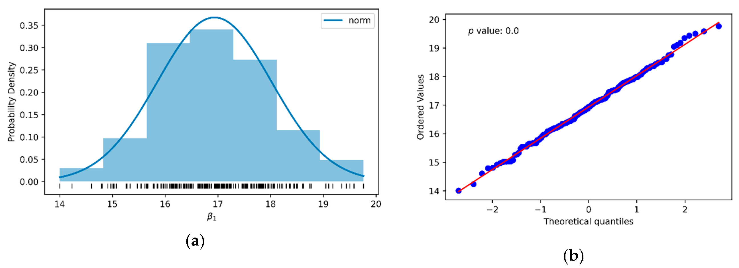
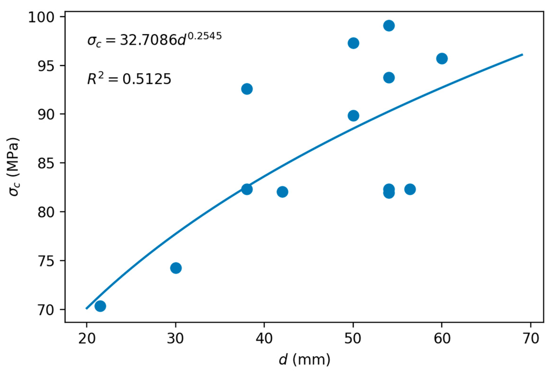
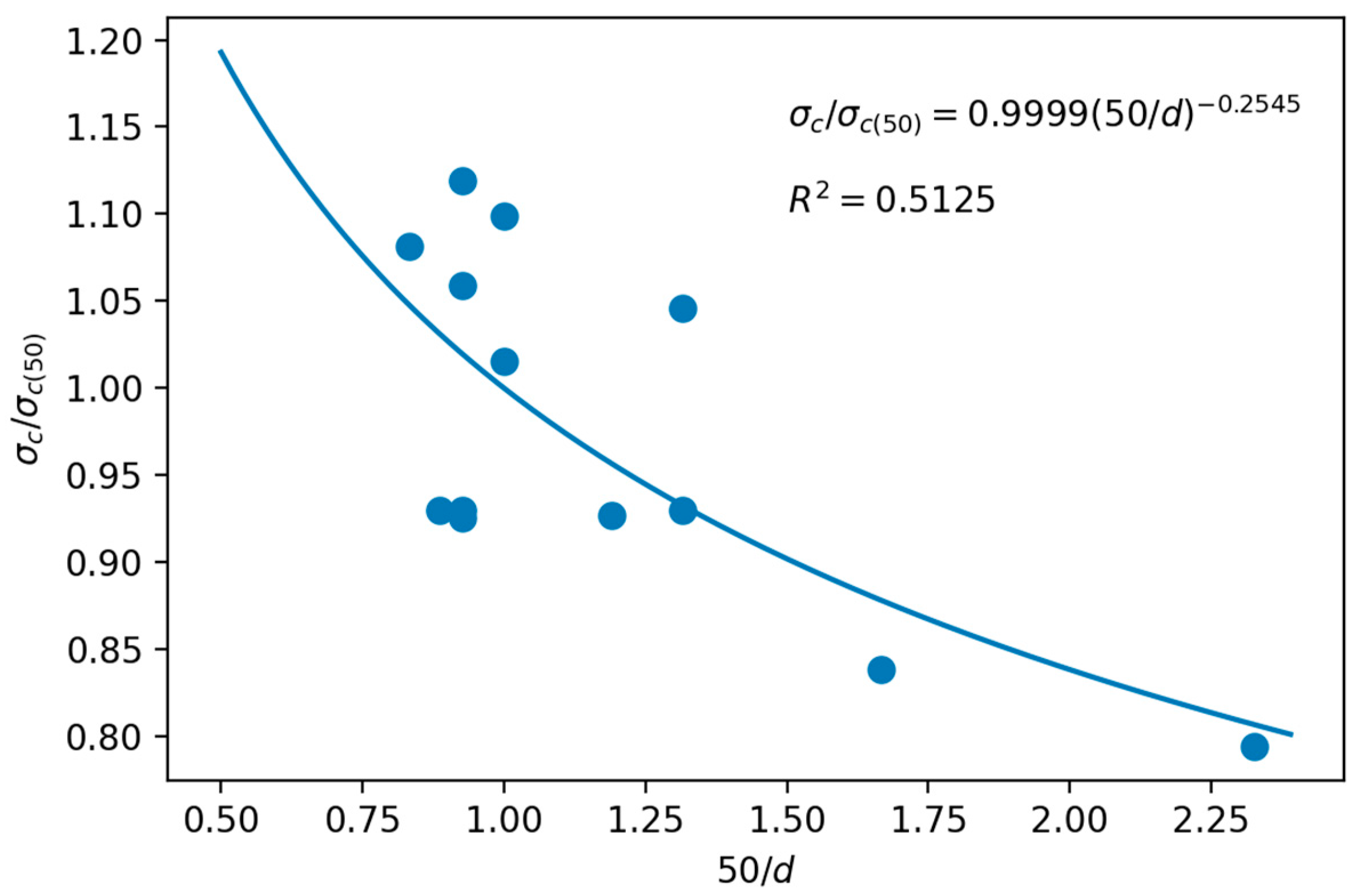
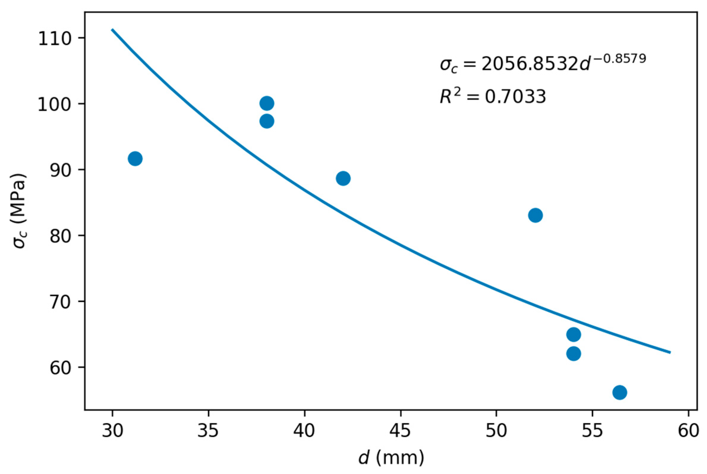
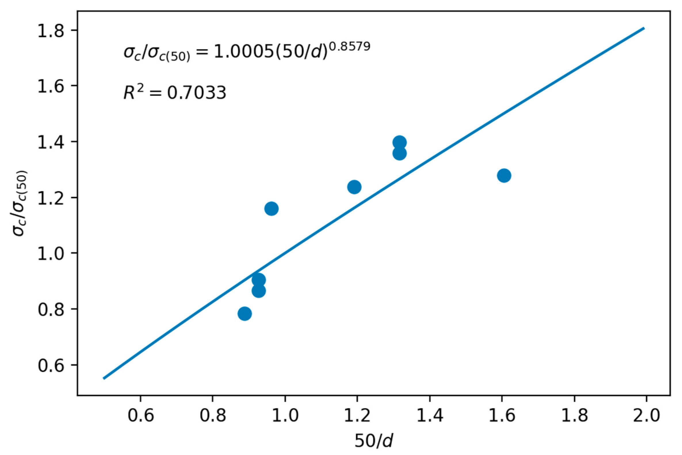
3.3. Scale Effect
3.3.1. Limestone
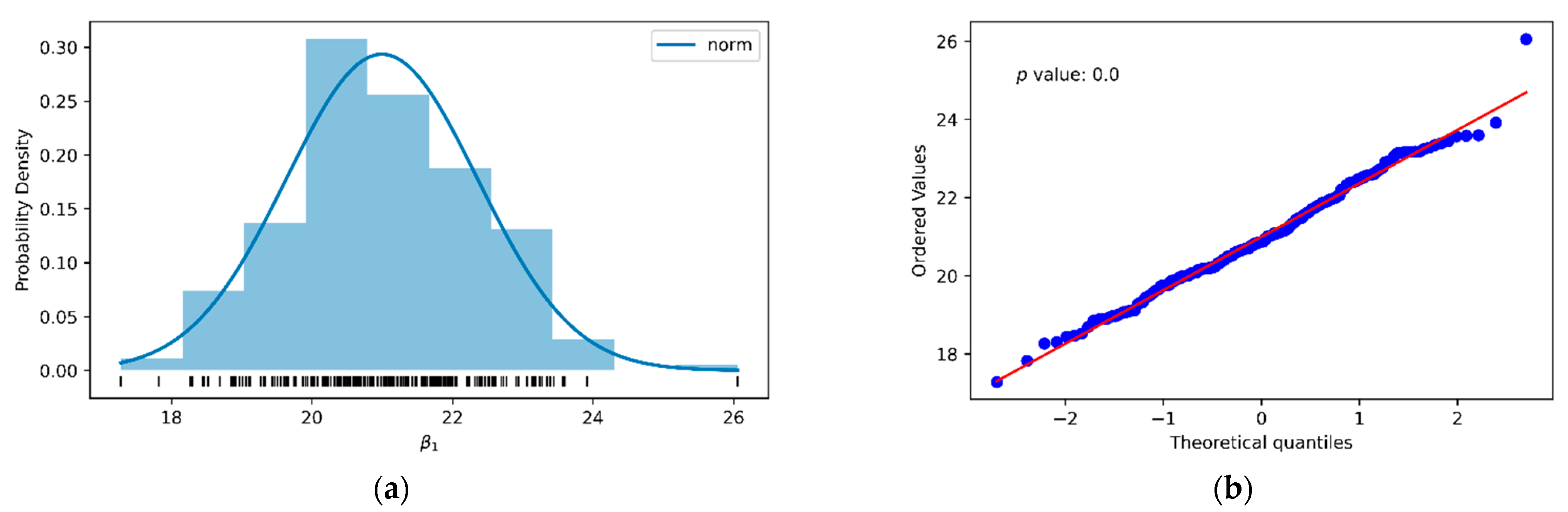
3.3.2. Travertine
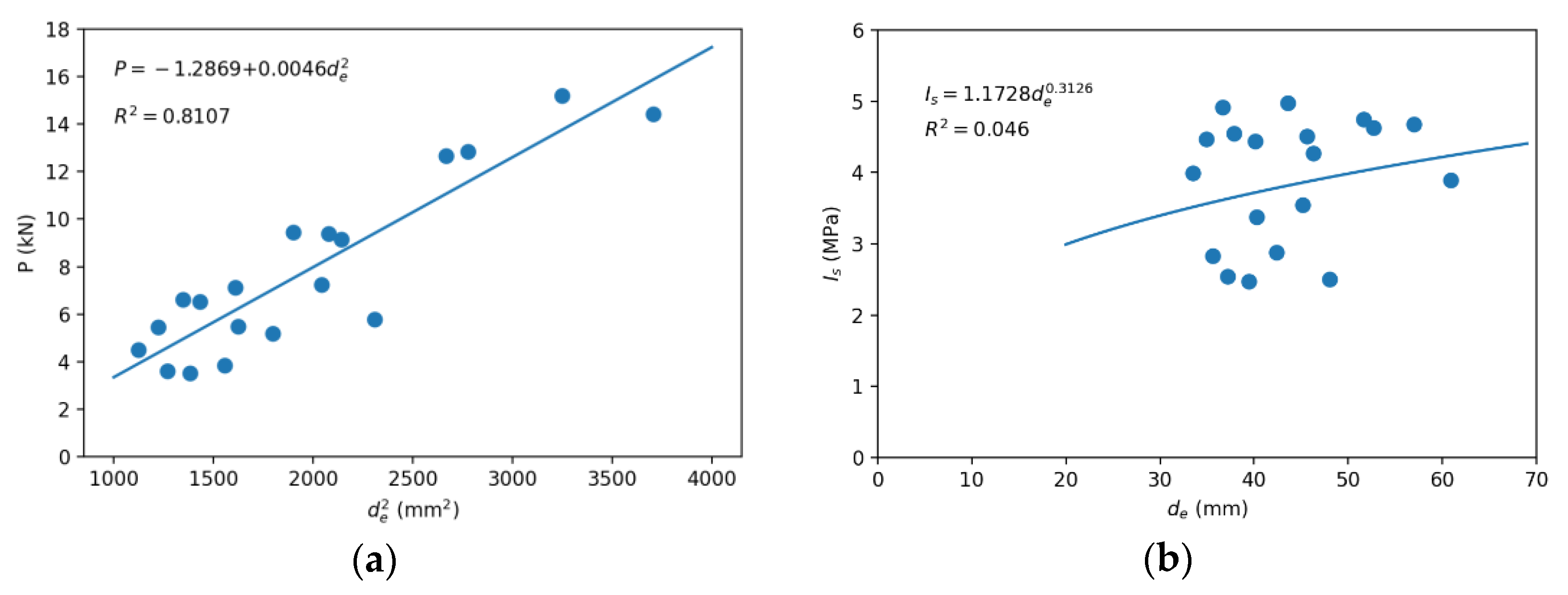
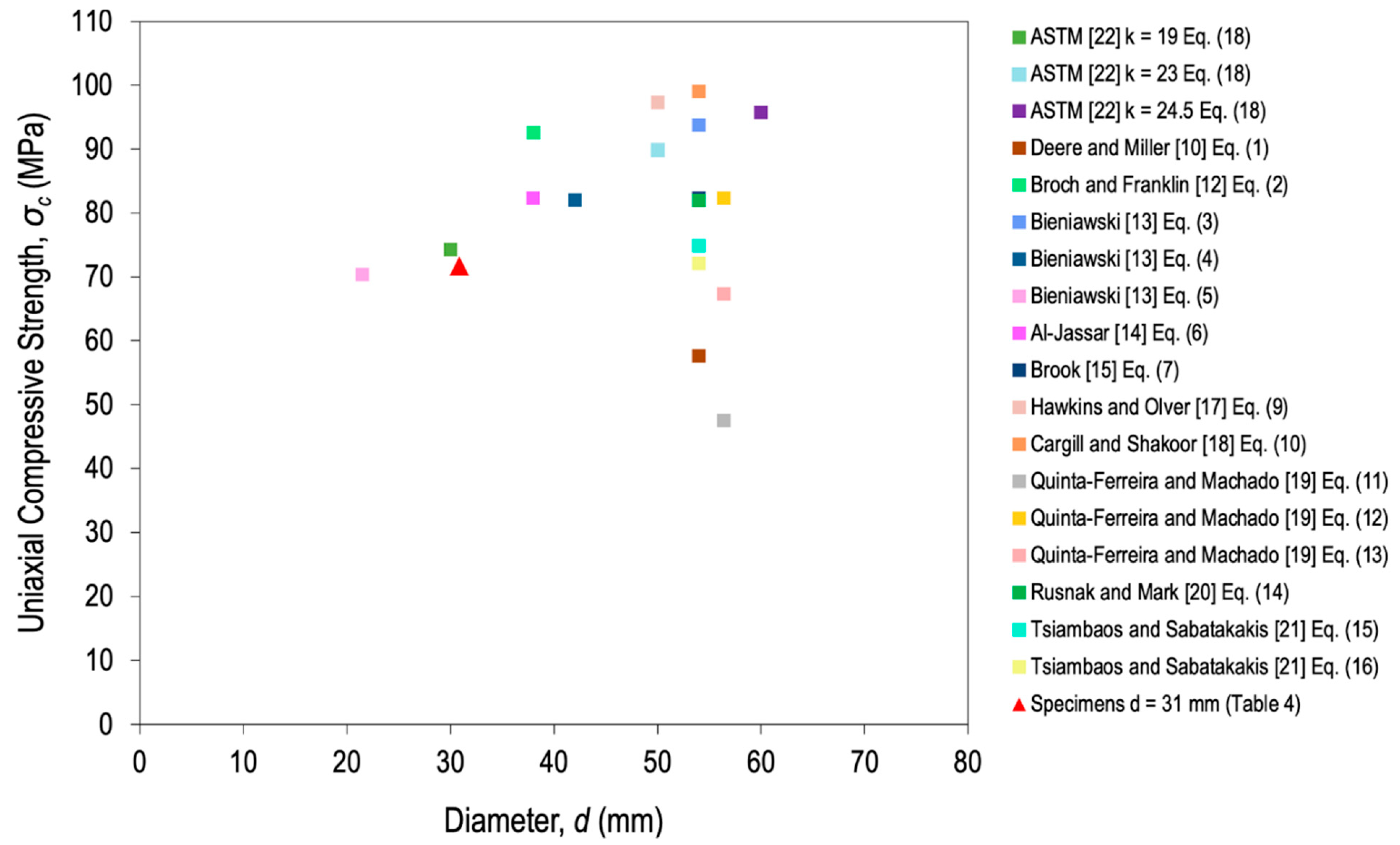
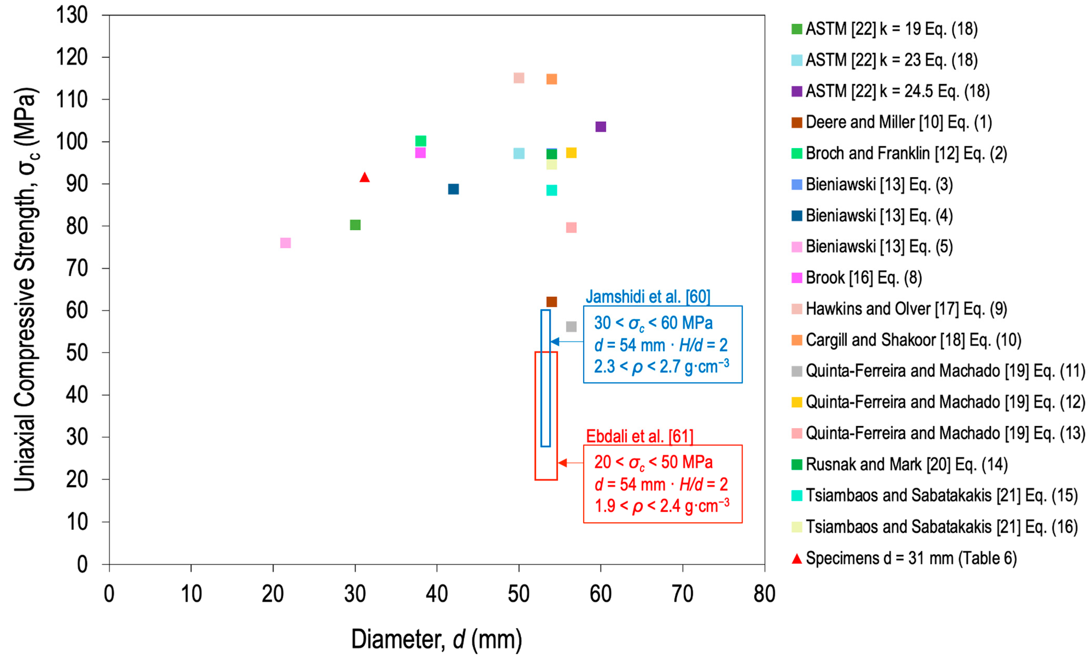
3.4. Correlation between Uniaxial Compressive Strength and Point Load Index
3.4.1. Limestone
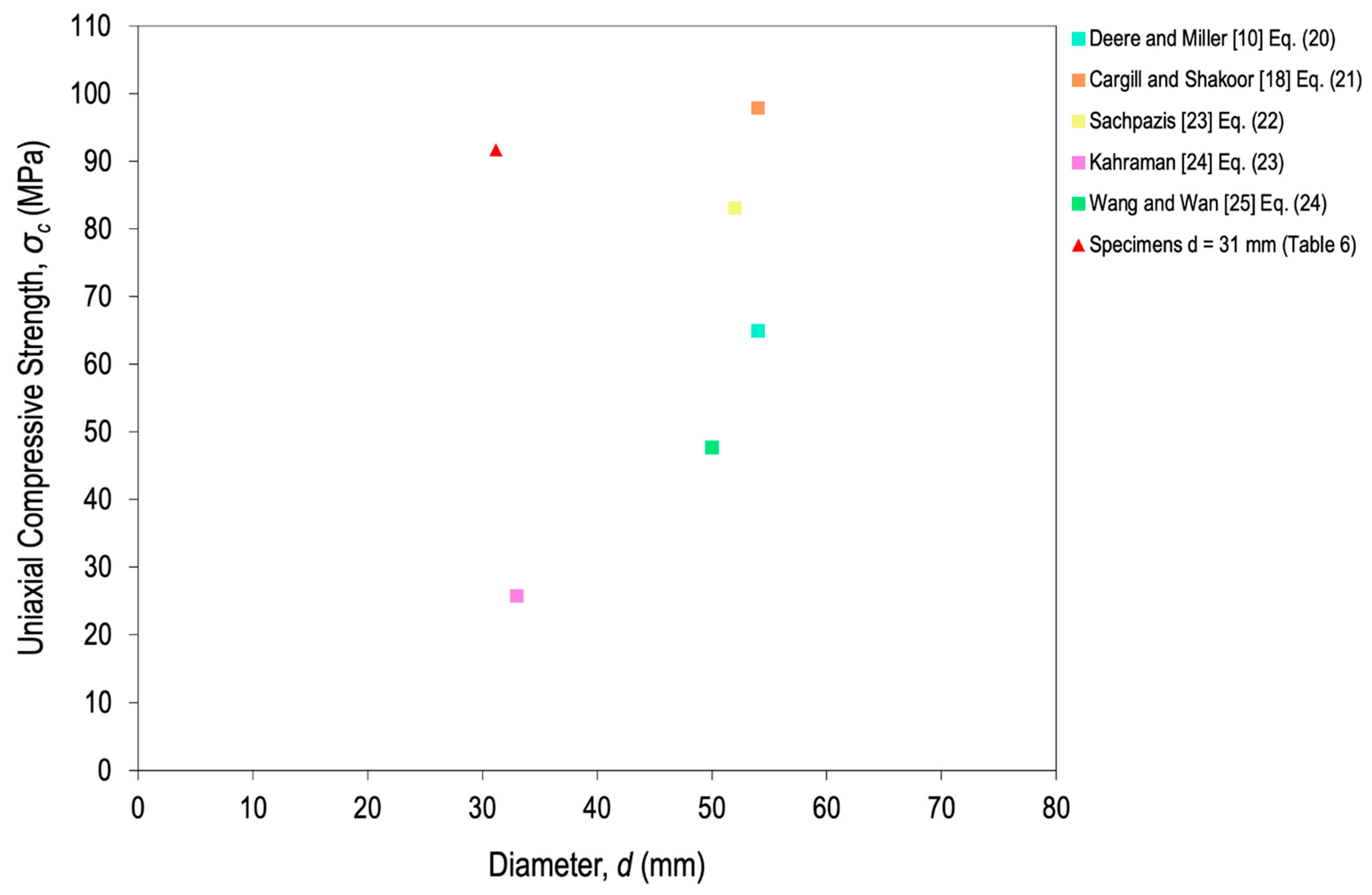
3.4.2. Travertine
4. Conclusions
Author Contributions
Funding
Institutional Review Board Statement
Informed Consent Statement
Acknowledgments
Conflicts of Interest
References
- ASTM D7012-14. Standard Test Method for Compressive Strength and Elastic Moduli of Intact Rock Core Specimens under Varying States of Stress and Temperatures; American Society for Testing and Materials: West Conshohocken, PA, USA, 2017; Available online: http://www.informationweek.com/news/201202317 (accessed on 2 April 2020).
- ASTM D4543-19. Standard Test Methods for Preparing Rock Core as Cylindrical Test Specimens and Verifying Conformance to Dimensional and Shape Tole-rances; American Society for Testing and Materials: West Conshohocken, PA, USA, 2019; Available online: http://www.informationweek.com/news/201202317 (accessed on 2 April 2020).
- ISRM. The Complete ISRM Suggested Methods for Rock Characterization, Testing and Monitoring: 1974–2006; ISRM Turkish National Group: Ankara, Turkey, 2007. [Google Scholar]
- Tugrul, A.; Zarif, H. Correlation of mineralogical and textural characteristics with engineering properties of selected granitic rocks from Turkey. Eng. Geol. 1999, 51, 303–317. [Google Scholar] [CrossRef]
- Kiliç, A.; Teymen, A. Determination of mechanical properties of rocks using simple methods. Bull. Eng. Geol. Environ. 2008, 67, 237–244. [Google Scholar] [CrossRef]
- Nabaei, M.; Shahbazi, K.; Shadravan, A.; Azad, I. Uncertainty Analysis in Unconfined Rock Compressive Strength Prediction. In Proceedings of the SPE Deep Gas Conference and Exhibition, Manama, Bahrein, 24–26 January 2010. SPE-131719-MS. [Google Scholar] [CrossRef]
- Török, Á.; Vásárhelyi, B. The influence of fabric and water content on selected rock mechanical parameters of travertine, examples from Hungary. Eng. Geol. 2010, 115, 237–245. [Google Scholar] [CrossRef]
- Rabbani, E.; Sharif, F.; Koolivand Salooki, M.; Moradzadeh, A. Application of neural network technique for prediction of uniaxial compressive strength using reservoir formation properties. Int. J. Rock Mech. Min. Sci. 2012, 56, 100–111. [Google Scholar] [CrossRef]
- Çelik, S.B. Prediction of uniaxial compressive strength of carbonate rocks from nondestructive tests using multivariate regression and LS-SVM methods. Arab. J. Geosci. 2019, 12, 193. [Google Scholar] [CrossRef]
- Deere, D.; Miller, R. Engineering Classification and Index Properties for Intact Rock; Technical Report No. AFWL-TR-65-116; Air Force Weapons Laboratory/Kirtland Air Base: Albuquerque, NM, USA, 1966. [Google Scholar]
- Vásárhelyi, B. Statistical Analysis of the Influence of Water Content on the Strength of the Mioecene Limestone. Rock Mech. Rock Eng. 2005, 38, 69–76. [Google Scholar] [CrossRef]
- Broch, E.; Franklin, J.A. The point load test. Int. J. Rock Mech. Min. Sci. Geomech. Abstr. 1972, 9, 669–697. [Google Scholar] [CrossRef]
- Bieniawski, Z.T. The point-load test in geotechnical practice. Eng. Geol. 1975, 9, 1–11. [Google Scholar] [CrossRef]
- Al-Jassar, S.H.; Hawkins, A.B. Geotechnical Properties of the Carboniferous Limestone of the Bristol Area the Influence of Petrography and Cheistry. In Proceedings of the 4th ISRM Congress, Montreux, Switzerland, 2–8 September 1979; pp. 1–14. [Google Scholar]
- Brook, N. Size correction for point load testing. Int. J. Rock Mech. Min. Sci. Geomech. Abstr. 1980, 17, 231–235. [Google Scholar] [CrossRef]
- Brook, N. The equivalent core diameter method of size and shape correction in point load testing. Int. J. Rock. Mech. Min. Sci. Geomech. Abstr. 1985, 22, 61–70. [Google Scholar] [CrossRef]
- Hawkins, A.B.; Olver, J.A.G. Point load tests: Correlation factors and contractual use. An example from the Corallian at Weymouth. Geol. Soc. Eng. Geol. Special Publ. 1986, 2, 269–271. [Google Scholar] [CrossRef]
- Cargill, J.S.; Shakoor, A. Evaluation of empirical methods for measuring the uniaxial compressive strength of rock. Int. J. Rock Mech. Min. Sci. Geomech. Abstr. 1990, 27, 495–503. [Google Scholar] [CrossRef]
- Quinta-Ferreira, M.O.; Machado, A.P.G. Assessing Limestone Strength with the Point Load Test. In Scale Effects in Rock Masses 93, Proceedings of the 2nd International Scale Effects in Rock Masses, Lisbon, Portugal, 25 June 1993; Pinto da Cunha, A., Ed.; CRC Press: Boca Raton, FL, USA, 1993. [Google Scholar]
- Rusnak, J.; Mark, C. Using the point load test to determine the uniaxial compressive strength of coal measure rock. In Proceedings of the 19th International Conference on Ground Control in Mining, Morgantown, WV, USA, 8–10 August 2000; Peng, S.S., Mark, C., Eds.; West Virginia University: Morgantown, WV, USA, 2000; pp. 362–371. [Google Scholar]
- Tsiambaos, G.; Sabatakakis, N. Considerations on strength of intact sedimentary rocks. Eng. Geol. 2004, 72, 261–263. [Google Scholar] [CrossRef]
- ASTM D5731-16. Standard Test Method for Determination of the Point Load Strength Index of Rock and Application to Rock Strength Classifications; American Society for Testing and Materials: West Conshohocken, PA, USA, 2016. [Google Scholar]
- Sachpazis, C. Correlating Schmidt hardness with compressive strength and Young’s modulus of carbonate rocks. Bull. Int. Assoc. Eng. Geol. 1990, 42, 75–83. [Google Scholar] [CrossRef]
- Kahraman, S. Evaluation of simple methods for assessing the uniaxial compressive strength of rock. Int. J. Rock Mech. Min. Sci. 2001, 38, 981–994. [Google Scholar] [CrossRef]
- Wang, M.; Wan, W. A new empirical formula for evaluating uniaxial compressive strength using the Schmidt hammer test. Int. J. Rock. Mech. Min. Sci. 2019, 123, 104094. [Google Scholar] [CrossRef]
- Wang, S.; Masoumi, H.; Oh, J.; Zhang, S. Scale-Size and Structural Effects of Rock Materials; Woodhead Publishing: London, UK, 2020. [Google Scholar]
- Mogi, K. Some precise measurements of fracture strength of rocks under uniform compressive stress. Rock Mech. Eng. Geol. 1966, 4, 41–55. [Google Scholar]
- Mogi, K. Experimental Rock Mechanics; Taylor & Francis: London, UK, 2007. [Google Scholar]
- John, M. The Influence of Length to Diameter Ratio on Rock Properties in Uniaxial Compression; A Contribution to Standardization in Rock Mechanics Testing; Report South African CSIR No ME1083/5; Council for Scientific and Industrial Research: Pretoria, South Africa, 1972; Available online: http://www.informationweek.com/news/201202317 (accessed on 2 April 2020).
- Fener, M. The Effect of Rock Sample Dimension on the P-Wave Velocity. J. Nondestr. Eval. 2011, 30, 99–105. [Google Scholar] [CrossRef]
- González, J.; Saldaña, M.; Arzúa, J. Analytical Model for Predicting the UCS from P-Wave Velocity, Density, and Porosity on Saturated Limestone. Appl. Sci. 2019, 9, 5265. [Google Scholar] [CrossRef] [Green Version]
- Saldaña, M.; González, J.; Pérez-Rey, I.; Jeldres, M.; Toro, N. Applying Statistical Analysis and Machine Learning for Modeling the UCS from P-Wave Velocity, Density and Porosity on Dry Travertine. Appl. Sci. 2020, 10, 4565. [Google Scholar] [CrossRef]
- Hoek, E.; Brown, E.T. Underground Excavations in Rock; Institution of Mining and Metallurgy: London, UK, 1980. [Google Scholar]
- Hoek, E.; Brown, E.T. Empirical Strength Criterion for Rock Masses. J. Geotech. Eng. Div. 1980, 106, 1013–1035. [Google Scholar] [CrossRef]
- D’Andrea, D.V.; Fisher, R.L.; Fogelson, D.E. Prediction of Compressive Strength of Rock from Other Rock Properties; USBM RI 6702; US Department of the Interior, Bureau of Mines: Washington, DC, USA, 1965.
- Deere, D.U. Geological considerations. In Rock Mechanics in Engineering Practice; Stagg, K.G., Zienkiewicz, D.C., Eds.; Wiley: London, UK, 1968. [Google Scholar]
- Aydin, A.; Basu, A. The Schmidt hammer in rock material characterization. Eng. Geol. 2005, 81, 1–14. [Google Scholar] [CrossRef]
- ISRM. The Complete ISRM Suggested Methods for Rock Characterization, Testing and Monitoring: 2007–2014; ISRM Turkish National Group: Ankara, Turkey, 2015. [Google Scholar]
- ASTM D5873-14. Standard Test Methods for Determination of Rock Hardness by Rebound Hammer Method; American Society for Testing and Materials: West Conshohocken, PA, USA, 2014. [Google Scholar]
- Weibull, W. A Statistical Theory of the Strength of Materials; Royal Swedish Academy of Engineering Science: Stockholm, Sweden, 1939. [Google Scholar]
- Weibull, W. A statistical distribution of function of wide applicability. ASME J. Appl. Mech. 1951, 18, 293–297. [Google Scholar] [CrossRef]
- Bieniawski, Z.T. The effect of specimen size on compressive strength of coal. Int. J. Rock Mech. Min. Sci. Geomech. Abstr. 1967, 5, 325–335. [Google Scholar] [CrossRef]
- Yoshinaka, R.; Osada, M.; Park, H.; Sasaki, T.; Sasaki, K. Practical determination of mechanical design parameters of intact rock considering scale effect. Eng. Geol. 2008, 96, 173–186. [Google Scholar] [CrossRef]
- Hawkins, A.B. Aspects of rock strength. Bull. Eng. Geol. Environ. 1998, 57, 17–30. [Google Scholar] [CrossRef]
- Bazant, Z.P. Size effect in blunt fracture: Concrete, rocks and metal. Eng. Mech. 1984, 110, 518–535. [Google Scholar] [CrossRef]
- Griffith, A.A. Theory of rupture. In Proceedings of the 1st International Congress for Applied Mechanics, Delft, The Netherland, 22–26 April 1924; pp. 55–63. [Google Scholar]
- Hudson, J.A.; Crouch, S.L.; Fairhurst, C. Soft, stiff and servo-controlled testing machines: A review with reference to rock failure. Eng. Geol. 1972, 6, 155–189. [Google Scholar] [CrossRef]
- Abou-Sayed, A.S.; Brechtel, C.E. Experimental investigation of the effects of size on the uniaxial compressive strength of Cedar City quartz diorite. In Proceedings of the 17th US Symposium on Rock Mechanics (USRMS), Snowbird, UT, USA, 25–27 August 1976; ARMA: Edwards, CO, USA, 1976; pp. 1–9. [Google Scholar]
- Bazant, Z.P. Scaling of quasibrittle fracture: Hypotheses of invasive and lacunar fractality, their critique and Weibull connection. Int. J. Fracture 1997, 83, 41–65. [Google Scholar] [CrossRef]
- Masoumi, H.; Saydam, S.; Hagan, P.C. Unified size-effect law for intact rock. Int. J. Geomech. 2015, 16, 04015059. [Google Scholar] [CrossRef]
- Basu, A.; Aydin, A. A method for normalization of Schmidt hammer rebound values. Int. J. Rock Mech. Min. Sci. 2004, 41, 1211–1214. [Google Scholar] [CrossRef]
- Goodman, R.E. Introduction to Rock Mechanics, 2nd ed.; Wiley: New York, NY, USA, 1989. [Google Scholar]
- Lama, R.D.; Vutukuri, V.S. Handbook on Mechanical Properties of Rocks, 2nd ed.; Trans Tech Publications: Clausthal-Zellerfiel, Germany, 1978. [Google Scholar]
- IAEG. Classification of rocks and soils for engineering geological mapping. Part 1: Rock and soil materials. Bull. Int. Assoc. Eng. Geol. 1979, 19, 364–371. [Google Scholar] [CrossRef]
- Zhang, L. Engineering Properties of Rocks, 2nd ed.; Butterworth-Heinemann: Amsterdam, The Netherlands, 2017. [Google Scholar]
- Ramírez-Oyanguren, P.; Alejano, L.R. Mecánica de Rocas: Fundamentos de Ingeniería de Taludes; Red DESIR: Madrid, Spain, 2008. [Google Scholar]
- García del Cura, M.; Benavente, D.; Martínez-Martínez, J.; Cueto, N. Sedimentary structures and physical properties of travertine and carbonate tufa building stone. Constr. Build. Mater. 2012, 28, 456–467. [Google Scholar] [CrossRef]
- Soete, J.; Kleipool, L.; Claes, H.; Claes, S.; Hamaekers, H.; Kele, S.; Swennen, R. Acoustic properties in travertines and their relation to porosity and pore types. Marine Petrol. Geol. 2015, 59, 320–335. [Google Scholar] [CrossRef] [Green Version]
- Yagiz, S. P-wave velocity test for assessment of geotechnical properties of some rock materials. Bull. Mater. Sci. 2011, 34, 947–953. [Google Scholar] [CrossRef]
- Jamshidi, A.; Nikudel, M.R.; Khamehchiyan, M.; Sahamieh, R.Z. The effect of specimen diameter size on uniaxial compressive strength P wave velocity and the correlation between them. Geomech. Geoeng. 2016, 11, 13–19. [Google Scholar] [CrossRef]
- Ebdali, M.; Khorasani, E.; Salehin, S. A comparative study of various hybrid neural networks and regression analysis to predict unconfined compressive strength of travertine. Innov. Infrastruct. Solut. 2020, 5, 93. [Google Scholar] [CrossRef]
- Walpole, R.; Myers, R.; Myers, S.; Ye, K. Probabilidad y Estadística para Ingeniería y Ciencias; Pearson: Ciudad de Mexico, México, 2012. [Google Scholar]


| Correlation | R2 | Rock Type | Geometry | Reference | Equation | |||
|---|---|---|---|---|---|---|---|---|
| σc | PLT * | |||||||
| Axial | Diametral | Blocks or Slumps | ||||||
| 0.92 | Basalt, diabase, dolomite, gneiss, granite, limestone, marble, quartzite, rock salt, sandstone, schist, siltstone, tuff | d = 54 mm H/d = 2 | - | d = 54 mm H/d = 2 | - | Deere and Miller [10] | (1) | |
| 0.88 | Dolerite, sandstone | d = 38 mm H/d = 2 | - | d = 38 mm (50 mm corrected)/L ≥ 0.7D/H/d > 1.4 | - | Broch and Franklin [12] | (2) | |
| - | Norite, quartzite, sandstone | d = 54 mm | - | d = 54 mm/L > 0.7D | - | Bieniawski [13] | (3) | |
| - | d = 42 mm | d = 42 mm/L > 0.7D | (4) | |||||
| - | d = 21.5 mm | d = 21.5 mm/L > 0.7D | (5) | |||||
| - | Dolomite, limestone, sandstone | d = 38 mm H = 76 mm | d = 50 mm (does not specify the type of test) | Al-Jassar [14] | (6) | |||
| - | Basalt, diabase, dolerite, norite, quartzite, sandstone, etc. | The data used to correlate σc and T500 are those of Broch and Franklin [12], Bieniawski [13], D’Andrea et al. [35], and Deere [36] | Brook [15] | (7) | ||||
| Brook [16] | (8) | |||||||
| - | Limestone | d = 50 mm H = 100 mm | d = 76‒92 mm corrected to 50 mm with Broch and Franklin [12] | - | Hawkins and Olver [17] | (9) | ||
| 0.94 | Dolomite, gneiss, limestone, marble, sandstone | d = 54 mm H/d = 2 | - | d = 50 mm H/d = 1.1 | - | Cargill and Shakoor [18] | (10) | |
| - | Dolomitic limestone | 5 × 5 × 10 cm3 (de = 56.4 mm) D/W = 1 | - | - | 10 × 10 × 20 cm3 (de = 112.8 mm) 5 × 5 × 10 cm3 (de = 56.4 mm) 2.5 × 2.5 × 5 cm3 (de = 28.2 mm) all corrected to d = 50 mm | Quinta-Ferreira and Machado [19] | (11) | |
| - | Micritic limestone | (12) | ||||||
| - | Mean correlation | (13) | ||||||
| - | Limestone | d = 54 mm (most) d = 75 mm (rest) | - | - | - | Rusnak and Mark [20] | (14) | |
| 0.40 | Calcareous-marly, limestone, marlstone, sandstone, quartzitic-greywacke | d = 54 mm H/d = 2–2.5 | - | d = 50 mm H = 110 mm | - | Tsiambaos and Sabatakakis [21] | (15) | |
| 0.82 | (16) | |||||||
| - | - | - | 0.3 < L/D < 1 | L/D > 1 L = 0.5D | 0.3 < D/W < 1 L/W > 0.5 | ISRM [3] | (17) | |
| - | - | - | 30 < d < 85 mm H/d = 0.3–1 0.3W > D > W | 30 < d < 85 mm H/d > 1 L = 0.5 | 0.3 < D/W < 1 L/W > 0.5 | ASTM [22] | (18) | |
| Correlation | R2 | Rock Type | Geometry σc | Geometry R * | Reference | Equation |
|---|---|---|---|---|---|---|
| - | Basalt, diabase, dolomite, gneiss, granite, limestone, marble, quartzite, rock salt, sandstone, schist, siltstone, tuff | d = 54 mm H/d = 2 | d = 54 mm H/d = 2 | Deere and Miller [10] | (20) | |
| - | Dolomite, gneiss, limestone, marble | d = 54 mm H/d = 2 | d = 54 mm 2 < H/d < 2.3 | Cargill and Shakoor [18] | (21) | |
| 0.92 | Dolomite, limestone, marble | d = 52 mm d = 38 mm | Blocks 25 × 25 × 20 cm3 | Sachpazis [23] | (22) | |
| 0.92 | Diabase, dolomite, marl, sandstone, serpentine, tuff | d = 33 mm H/d = 2 | - | Kahraman [24] | (23) | |
| 0.92 | Granite, limestone, sandstone | d = 50 mm H = 100 mm | 10 ≤ RL ≤ 70 | Wang and Wan [25] | (24) |
| Diameter, d (mm) | F |
|---|---|
| 21.5 | 18 |
| 30 | 19 |
| 42 | 21 |
| 50 | 23 |
| 54 | 24 |
| 60 | 24.5 |
| Specimen | d (mm) | H (mm) | neff (%) | ρsat (g·cm–3) | σc (MPa) |
|---|---|---|---|---|---|
| Limestone 1 | 30.830 | 60.548 | 2.46 | 2.66 | 76.30 |
| Limestone 2 | 30.853 | 60.335 | 3.15 | 2.62 | 41.37 |
| Limestone 3 | 30.968 | 60.135 | 2.26 | 2.63 | 77.59 |
| Limestone 4 | 30.860 | 60.588 | 1.95 | 2.64 | 106.19 |
| Limestone 5 | 30.923 | 60.345 | 2.55 | 2.61 | 77.10 |
| Limestone 6 | 30.858 | 60.718 | 2.46 | 2.65 | 91.43 |
| Limestone 7 | 30.933 | 60.395 | 2.43 | 2.62 | 55.93 |
| Limestone 8 | 30.193 | 60.650 | 2.29 | 2.64 | 73.14 |
| Limestone 9 | 30.843 | 59.855 | 3.27 | 2.60 | 49.24 |
| Limestone 10 | 30.853 | 60.518 | 2.95 | 2.61 | 42.15 |
| Limestone 11 | 30.975 | 60.155 | 2.26 | 2.68 | 61.24 |
| Limestone 12 | 30.808 | 60.223 | 2.32 | 2.63 | 94.32 |
| Limestone 13 | 30.915 | 60.458 | 2.77 | 2.62 | 50.80 |
| Mean | 30.832 | 60.379 | 2.55 | 2.63 | 68.99 |
| SD | 0.199 | 0.241 | 0.384 | 0.02 | 20.77 |
| Slump | D (mm) | W (mm) | de (mm) | P (kN) | Is (MPa) | Is(50) (MPa) |
|---|---|---|---|---|---|---|
| Limestone 1 | 18 | 55.38 | 35.6 | 3.598 | 2.83 | 2.55 |
| Limestone 2 | 22 | 57.4 | 40.1 | 7.135 | 4.44 | 4.14 |
| Limestone 3 | 22 | 64.18 | 42.4 | 5.175 | 2.88 | 2.73 |
| Limestone 4 | 22 | 57.95 | 40.3 | 5.49 | 3.38 | 3.16 |
| Limestone 5 | 30 | 32 | 35.0 | 5.459 | 4.47 | 3.99 |
| Limestone 6 | 29 | 56.3 | 45.6 | 9.376 | 4.51 | 4.38 |
| Limestone 7 | 30 | 49.75 | 43.6 | 9.459 | 4.98 | 4.77 |
| Limestone 8 | 42 | 69.28 | 60.9 | 14.423 | 3.89 | 4.14 |
| Limestone 9 | 38 | 67.13 | 57.0 | 15.2 | 4.68 | 4.88 |
| Limestone 10 | 40 | 52.35 | 51.6 | 12.662 | 4.75 | 4.80 |
| Limestone 11 | 39 | 55.9 | 52.7 | 12.845 | 4.63 | 4.70 |
| Limestone 12 | 30 | 53.48 | 45.2 | 7.235 | 3.54 | 3.43 |
| Limestone 13 | 22 | 48.05 | 36.7 | 6.614 | 4.91 | 4.46 |
| Limestone 14 | 39 | 43.1 | 46.3 | 9.152 | 4.28 | 4.17 |
| Limestone 15 | 42 | 43.15 | 48.0 | 5.776 | 2.50 | 2.47 |
| Limestone 16 | 23 | 47.18 | 37.2 | 3.512 | 2.54 | 2.32 |
| Limestone 17 | 31 | 39.43 | 39.5 | 3.848 | 2.47 | 2.30 |
| Limestone 18 | 21 | 42.03 | 33.5 | 4.492 | 4.00 | 3.53 |
| Limestone 19 | 27 | 41.65 | 37.8 | 6.514 | 4.55 | 4.17 |
| Specimen | d (mm) | H (mm) | neff (%) | ρdry (g⋅cm–3) | σc (MPa) |
|---|---|---|---|---|---|
| Travertine 1 | 31.090 | 59.470 | 3.65 | 2.48 | 75.28 |
| Travertine 2 | 30.970 | 59.550 | 4.09 | 2.37 | 74.95 |
| Travertine 3 | 31.000 | 60.350 | 4.44 | 2.37 | 97.55 |
| Travertine 4 | 30.750 | 60.350 | 4.58 | 2.36 | 89.79 |
| Travertine 5 | 31.050 | 60.160 | 3.58 | 2.38 | 54.17 |
| Travertine 6 | 31.080 | 60.310 | 4.57 | 2.47 | 78.43 |
| Travertine 7 | 31.170 | 59.980 | 4.70 | 2.41 | 93.17 |
| Travertine 8 | 31.118 | 59.688 | 4.37 | 2.48 | 74.79 |
| Travertine 9 | 31.070 | 59.780 | 7.19 | 2.41 | 78.84 |
| Travertine 10 | 31.020 | 59.800 | 6.65 | 2.40 | 85.98 |
| Travertine 11 | 31.175 | 61.613 | 4.92 | 2.47 | 63.78 |
| Travertine 12 | 31.213 | 62.450 | 4.71 | 2.46 | 104.00 |
| Travertine 13 | 31.200 | 62.900 | 3.83 | 2.45 | 121.98 |
| Travertine 14 | 31.200 | 61.950 | 4.00 | 2.41 | 81.91 |
| Travertine 15 | 31.187 | 62.000 | 4.12 | 2.44 | 94.61 |
| Travertine 16 | 31.250 | 61.663 | 4.61 | 2.41 | 88.86 |
| Travertine 17 | 31.163 | 61.938 | 8.01 | 2.34 | 85.65 |
| Travertine 18 | 31.200 | 61.950 | 7.34 | 2.40 | 50.89 |
| Travertine 19 | 31.300 | 62.650 | 3.43 | 2.42 | 98.26 |
| Travertine 20 | 31.250 | 61.925 | 3.68 | 2.45 | 84.71 |
| Travertine 21 | 31.150 | 62.450 | 5.42 | 2.37 | 81.05 |
| Travertine 22 | 31.150 | 62.350 | 2.32 | 2.41 | 123.38 |
| Travertine 23 | 31.220 | 62.300 | 4.19 | 2.37 | 90.77 |
| Travertine 24 | 31.100 | 62.650 | 4.71 | 2.45 | 88.17 |
| Travertine 25 | 31.200 | 62.250 | 1.05 | 2.49 | 115.430 |
| Travertine 26 | 31.400 | 62.100 | 0.99 | 2.47 | 129.170 |
| Travertine 27 | 31.400 | 62.200 | 0.77 | 2.46 | 115.560 |
| Travertine 28 | 31.200 | 62.700 | 0.72 | 2.50 | 125.870 |
| Travertine 29 | 31.250 | 62.500 | 0.70 | 2.43 | 112.870 |
| Mean | 31.128 | 61.259 | 4.05 | 2.43 | 91.72 |
| SD | 0.116 | 1.192 | 1.924 | 0.044 | 20.44 |
| Slump | D (mm) | W (mm) | de (mm) | P (kN) | Is (MPa) | Is(50) (MPa) |
|---|---|---|---|---|---|---|
| Travertine 30 | 46 | 74.5 | 66.1 | 16.6 | 3.80 | 4.15 |
| Travertine 31 | 57 | 99 | 84.8 | 22.8 | 3.17 | 3.74 |
| Travertine 32 | 36 | 47.5 | 46.7 | 12.2 | 5.60 | 5.48 |
| Travertine 33 | 45 | 56 | 56.6 | 15.7 | 4.89 | 5.09 |
| Travertine 34 | 41 | 78.1 | 63.9 | 14.1 | 3.46 | 3.73 |
| Travertine 35 | 48 | 64.5 | 62.8 | 16.3 | 4.14 | 4.44 |
| Travertine 36 | 39 | 101 | 70.8 | 12.4 | 2.47 | 2.76 |
| Travertine 37 | 42 | 53.5 | 53.5 | 12.3 | 4.30 | 4.39 |
| Travertine 38 | 39 | 59.5 | 54.4 | 16.3 | 5.52 | 5.66 |
| Travertine 39 | 32.2 | 61.3 | 50.1 | 12.4 | 4.93 | 4.94 |
| Travertine 40 | 39 | 67.9 | 58.1 | 15.6 | 4.63 | 4.85 |
| Travertine 41 | 36 | 74 | 58.2 | 15.9 | 4.69 | 4.92 |
| Travertine 42 | 43 | 70.8 | 62.3 | 13.1 | 3.38 | 3.62 |
| Travertine 43 | 25 | 80.6 | 50.7 | 10.7 | 4.17 | 4.19 |
| Sample | RN (no.) | |||||||||
|---|---|---|---|---|---|---|---|---|---|---|
| 1 | 2 | 3 | 4 | 5 | 6 | 7 | 8 | 9 | 10 | |
| 1 | 40 | 47 | 42 | 37 | 45 | 40 | 42 | 38 | 35 | 38 |
| 2 | 40 | 45 | 49 | 50 | 48 | 44 | 56 | 47 | 44 | 45 |
| 3 | 40 | 44 | 48 | 50 | 47 | 45 | 42 | 40 | 40 | 44 |
| Parameter | N | Mean | Standard Deviation | Maximum | Minimum |
|---|---|---|---|---|---|
| β1 | 200 | 16.93 | 1.09 | 19.76 | 14.00 |
| Parameter | N | Mean | Standard Deviation | Maximum | Minimum |
|---|---|---|---|---|---|
| β1 | 200 | 21.00 | 1.36 | 26.06 | 17.28 |
| Parameter | N | Mean | Standard Deviation | Maximum | Minimum |
|---|---|---|---|---|---|
| β1 | 200 | 20.64 | 1.21 | 25.78 | 17.75 |
| Parameter | N | Mean | Standard Deviation | Maximum | Minimum |
|---|---|---|---|---|---|
| β1 | 200 | 13.445 | 0.85 | 16.18 | 10.96 |
Publisher’s Note: MDPI stays neutral with regard to jurisdictional claims in published maps and institutional affiliations. |
© 2021 by the authors. Licensee MDPI, Basel, Switzerland. This article is an open access article distributed under the terms and conditions of the Creative Commons Attribution (CC BY) license (https://creativecommons.org/licenses/by/4.0/).
Share and Cite
Contreras, S.; Saldaña, M.; Toro, N.; Pérez-Rey, I.; González, M.A.; González, J. Scale Effect and Correlation between Uniaxial Compressive Strength and Point Load Index for Limestone and Travertine. Appl. Sci. 2021, 11, 3672. https://doi.org/10.3390/app11083672
Contreras S, Saldaña M, Toro N, Pérez-Rey I, González MA, González J. Scale Effect and Correlation between Uniaxial Compressive Strength and Point Load Index for Limestone and Travertine. Applied Sciences. 2021; 11(8):3672. https://doi.org/10.3390/app11083672
Chicago/Turabian StyleContreras, Solange, Manuel Saldaña, Norman Toro, Ignacio Pérez-Rey, Manuel A. González, and Javier González. 2021. "Scale Effect and Correlation between Uniaxial Compressive Strength and Point Load Index for Limestone and Travertine" Applied Sciences 11, no. 8: 3672. https://doi.org/10.3390/app11083672