Article

Exploring 3D Wave-Induced Scouring Patterns around Subsea Pipelines with Artificial Intelligence Techniques

by
Mohammad Najafzadeh
1,* and
Giuseppe Oliveto
2
1
Department of Water Engineering, Faculty of Civil and Surveying Engineering, Graduate University of Advanced Technology, Kerman 76315-117, Iran
2
School of Engineering, University of Basilicata, Viale dell’Ateneo Lucano 10, I-85100 Potenza, Italy
*
Author to whom correspondence should be addressed.
Appl. Sci. 2021, 11(9), 3792; https://doi.org/10.3390/app11093792
Submission received: 15 March 2021 / Revised: 9 April 2021 / Accepted: 14 April 2021 / Published: 22 April 2021
(This article belongs to the Special Issue Machine Learning Algorithms for Hydraulic Engineering)

Abstract

:

Featured Application

The paper presents new equations for predicting 3D scouring patterns at subsea pipelines under wave-only conditions. These equations are more reliable than conventional approaches and exhibit a clear physical consistence.

Abstract

Subsea pipelines carry oil or natural gas over long distances of the seabed, but fluid leakage due to a failure of the pipeline can culminate in huge environmental disasters. Scouring process may take place beneath pipelines due to current and/or wave action, causing pipeline suspension and leading to the risk of pipeline failure. The resulting morphological variations of the seabed propagate not only below and normally to the pipeline but also along the pipeline itself. Therefore, 3D scouring patterns need to be considered. Mainly based on the experimental works at laboratory scale by Cheng and coworkers, in this study, Artificial Intelligent (AI) techniques are employed to present new equations for predicting three dimensional current- and wave-induced scour rates around subsea pipelines. These equations are given in terms of key dimensionless parameters, among which are the Shields’ parameter, the Keulegan–Carpenter number, relative embedment depth, and wave/current angle of attach. Using various statistical benchmarks, the efficiency of AI-models-based regression equations is assessed. The proposed predictive models perform much better than the existing empirical equations from literature. Even more interestingly, they exhibit a clear physical consistence and allow for highlighting the relative importance of the key dimensionless variables governing the scouring patterns.

1. Introduction

Seabed pipelines are imperative to transport oil and gas from offshore platforms. Oil leakage due to failure of pipeline causes environmental disasters, which influence economic circumstances of nations. The flow structure of vortex around pipeline leads to vibration and consequently metal fatigue, which is introduced as one of the most commonly reported factors of pipeline failure. The scouring process may take place beneath pipelines when these offshore structures encounter rigorous oceanic flow (i.e., currents or waves). Longitudinal extension of the scour hole beneath the pipeline is inextricably bound to the pipeline span leading to pipeline spanning. When the extension of free span has sufficient extension in the longitudinal direction, seabed pipelines may experience severe vibration due to the existence of vortex structures (Xie and Zhu [1]).
For almost half a century, the scouring process below pipelines has been drawing meticulous attention by ocean and costal engineers in terms of safety of offshore structures. The scour hole around a pipeline is characterized by three-dimensional development due to the existence of the piping mechanism and an uneven seabed after the pipeline operation. When the scour hole grows longitudinally around the pipeline, the structure of free spans is developed. Basically, fully developed free spans are the main reason that pipelines are put into a failure state. In this case, the failure of pipelines is due to the fact that they are more exposed to structural destructions corresponding to over-stressing circumstances. The earliest experimental investigations proved that the formation of three-dimensional free spans around pipelines are efficient to augment the instability level of the pipeline. In addition to this, free spans can lead to natural self-burial into the scour hole formed below the pipeline (Sumer and Fredsøe [2]). Figure 1 shows the structure of free spans in the extension state. The propagation of the scour rate was seen in two opposite directions along the pipeline. Three-dimensional growth of the free span depends on the conditions of flow and sediment motion and pipeline geometry.
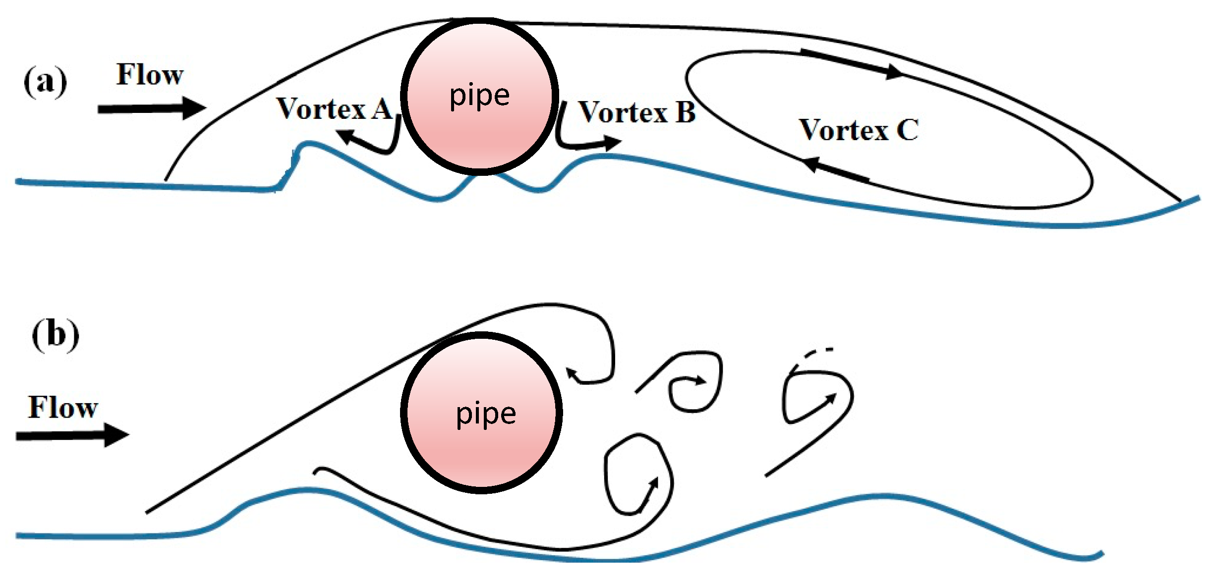
Figure 2 shows schematic diagrams of vortex structures around submarine pipelines under currents. Figure 2a illustrates three types of vortex structures. In the near vicinity of the pipeline, both vortices A and C move particles of bed sediments away from the footing area, even though movements of particles occur in opposite directions to each other. Vortex B also moves particles of bed sediment, but its acting area is constrained by Vortex C. Ultimately, a small opening is formed beneath the pipeline, which is introduced as the onset of unidirectional flow-induced scour. Figure 2b shows that as the water flows beneath the pipeline, the upstream vortex disappears, creating tunnel erosion gradually.
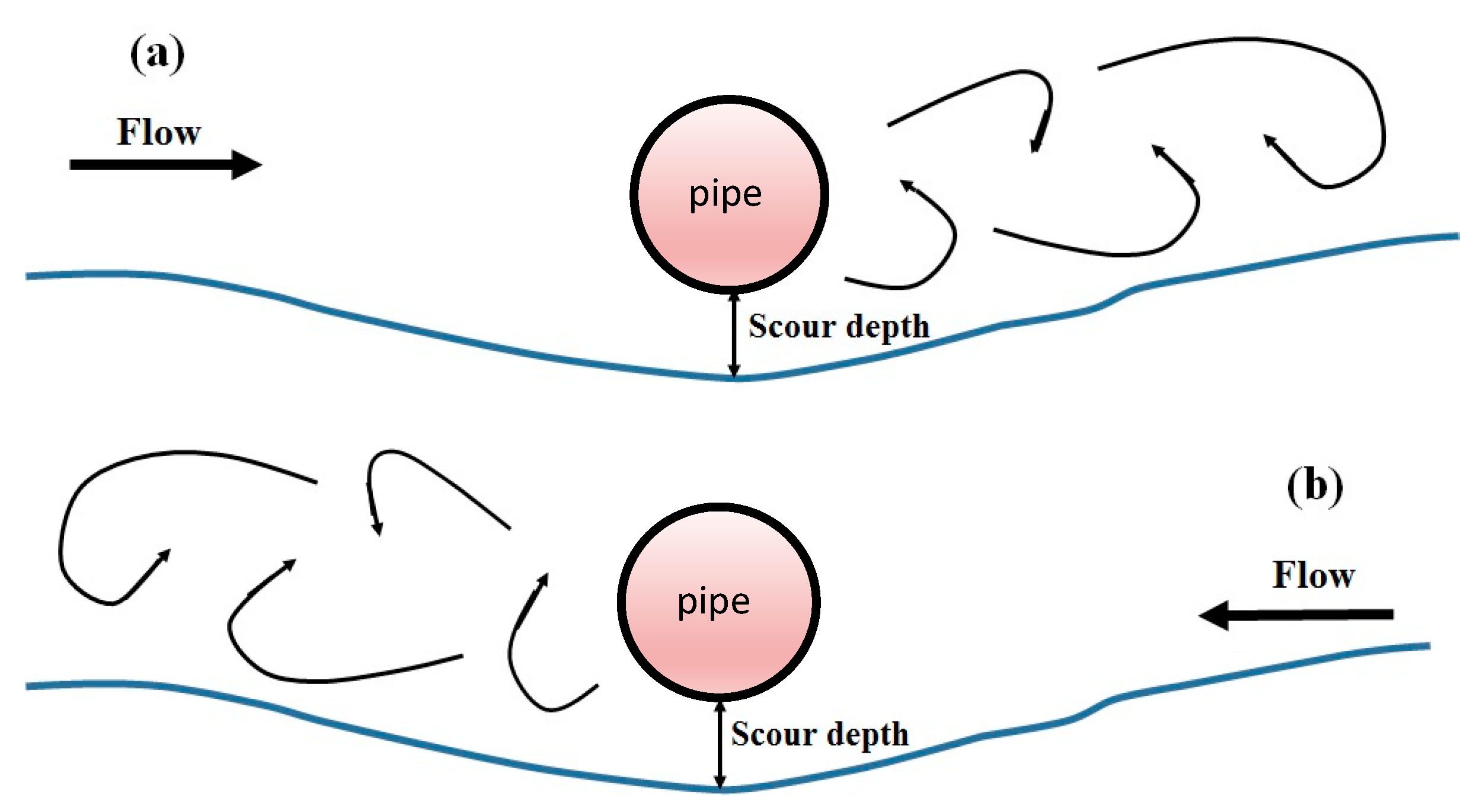
Figure 3 shows schematic diagrams of vortex structures around submarine pipelines under waves. As the full development of the scour hole is met, complicated flow structure of vortex shedding occurs behind the pipeline (Çevik and Yüksel [3]). As the flow structure has oscillatory pattern, a vortex system with wake intensity occurs on both sides of the pipeline. Figure 3 also shows the flow structure of lee-wake erosion, which takes place on both sides of the pipeline.
A large number of experimental studies have been carried out to better understand scouring mechanisms at submarine pipelines; the papers from [4,5,6,7,8,9,10,11,12,13,14] in the references section are some examples. Generally, all the experimental studies were carried out in three distinctive flow conditions: (1) Current, (2) regular wave, and (3) combined current and wave. Cheng et al. [6] investigated three-dimensional scour rates below a pipeline exposed to currents. They proposed an empirical equation for the prediction of longitudinal scour rates below the pipeline. Additionally, Cheng et al. [9] studied the scouring mechanism below a pipeline in two various flow conditions (i.e., combined wave and current, wave only). They proposed two regression-based equations for the prediction of the longitudinal scour rate in both flow conditions. In terms of the propagation of scour rates around pipelines, it can be inferred that there is limited knowledge on the scour hole development.
Previous attempts generally indicated that empirical equations are restricted to the range of experimental databases. Thus, these equations often do not have high potential of generalizing the prediction of scour rates in the three-dimensional space below pipelines.
In the case of experimental investigations, it may be expected to find comprehensive influences of various parameters on the scouring process below pipelines. An understanding of the free span propagation still requires in-depth investigations (Sumer and Fredsøe [2], Cheng et al. [6], Cheng et al. [9]).
With the advent of soft computing techniques, complicated mechanisms of real-life problems have become more understandable than before. In this way, there is a high demand for the presentation of robust mathematical models on the basis of Artificial Intelligent (AI) techniques in various fields of science. Over the last decade, a large number of AI approaches have been employed prosperously to obtain an accurate estimation of the local scour depth below pipelines exposed to currents and regular waves. In fact, Artificial Neural Networks (ANNs) (Azamathulla and Zakaria [15], Etemad-Shahidi et al. [16]), Adaptive Neuro-Fuzzy Inference Systems (ANFIS) (Zanganeh et al. [17]), Support Vector Machine (SVM) (Parsaie et al. [18]), Classification and Regression Tree (CART) (Etemad-Shahidi et al. [16], Yasa and Etemad-Shahidi [19]), Linear Genetic Programming (LGP), Gene-Expression Programming (GEP) (Azamathulla and Yusoff [20], Najafzadeh and Sarkamaryan [21]), Genetic Programming (GP) (Azamathulla and Ghani [22]), Group Method of Data Handling (GMDH) (Najafzadeh et al. [23], Najafzadeh et al. [24]), Multivariate Adaptive Regression Splines (MARS) (Haghiabi [25]), and Evolutionary Polynomial Regression (EPR) (Najafzadeh and Sarkamaryan [21]) proved to be successful applications. In the case of scour rates prediction, there have been a few endeavors to estimate three-dimensional free spans via GMDH and ANN models below a pipeline exposed to regular waves (Najafzadeh and Saberi-Movahed [26], Ehteram et al. [27]).
However, few investigations have been conducted to estimate scour propagation rates at seabed pipelines by AI models. In fact, the experimental detection of three-dimensional scour rates is generally expensive due to the need of advanced sensors and other facilities. To the best of the authors’ knowledge, powerful AI techniques such as MARS, GEP, and MT have not yet been applied in the prediction of scour propagation rates around seabed pipelines exposed to regular waves. As main merits, these AI techniques have potential in three main areas: (i) Presenting (non-linear) explicit equations for limited number of data; (ii) reducing the number of influential variables; and (iii) preserving the physical consistency of the generated models. The present paper moves in these directions, identifying new equations to predict 3D scour patterns at seabed pipelines depending on key dimensionless parameters. These equations would be more reliable than conventional approaches, as well as preserving physical consistency.

2. AI Predictive Techniques on Scouring below Seabed Pipeline: A Brief Review

This section provides a brief review on the literature studies in which scouring below seabed pipeline is addressed by AI techniques. The section is divided into two parts for the sake of clarity depending on whether scour is due to currents or waves.

2.1. Current-Induced-Pipeline Scour

In the case of pipeline scour due to currents, a large number of investigations was attempted to use various AI models along with preservation of scouring conceptions.
Azamathulla and Ghani [22] applied GP model to experimental datasets, which were extracted from two various flow and sediment conditions. Ultimately, they proposed a regression-based equation, which applies to both clear-water (CW) and live-bed (LB) conditions. However, two major drawbacks arise from their research work. In the first place, they should have separated the entire dataset into two basic sections depending on whether the scouring process was governed by clear-water or live-bed approach flow conditions. It is well known that these two regimes imply different scouring processes. Incidentally, Azamathulla and Ghani [22] did not consider the ratio e/D of the pipeline embedment depth e to the pipeline diameter D as a controlling variable in modeling live-bed conditions; and the reason is that e/D in the experiments made by Moncada and Aguirre [28], to which Azamathulla and Ghani [22] relate, was kept constant for live-bed conditions. The second drawback of the study by Azamathulla and Ghani [22] is that they considered the Reynolds number as the controlling variable of local scour depth, though approach flows were fully turbulent. These issues cause some concerns on the use of the equation developed by Azamathulla and Ghani [22] in practical applications. Azamathulla et al. [29] later employed the LGP technique to provide an empirical equation by still considering the same current-induced scour datasets. However, the equation given by LGP is also undermined by the same drawbacks as for Azamathulla and Ghani [22]. The same comments would apply to the study by Azamathulla and Zakaria [15], though they applied ANN models.
Zanganeh et al. [17] improved the ANFIS model by using Particle Swarm Optimization (PSO) to predict the local scour depth around seabed pipelines due to currents. However, the experimental datasets used in their study were released from a few studies with limited ranges for the governing variables. Furthermore, they did not always consider turbulent flows (i.e., flows independent from Reynolds number) during the development of the ANFIS-PSO models. Similarly, Azamathulla and Yusoff [20] proposed a regression-based formulation by means of GEP technique. It looks like also their research did not follow physical insights of scouring mechanisms in terms of sediment bed motion and turbulent flow circumstances. Najafzadeh et al. [23] applied the GMDH technique to predict the local scour for various sediment motion conditions of approach flows. They not only enhanced existing inaccuracies in the literature, but also covered fundamental misconceptions related to the physical insights of scouring processes in similar previous investigations. They concluded that the performance of GMDH was relatively more accurate than SVM technique.
Yasa and Etemad-Shahidi [19] presented the CART-model-based probabilistic framework for various levels of risk in the design of undersea pipelines. They propose a regression equation, based on experimental data, for the economic design of a pipeline due to scour depth. Haghiabi [25] used the MARS technique to provide a robust formulation for the estimation of scour depth below pipelines exposed to clear-water circumstances. He found that MARS model was more accurate than the ANN technique and empirical equations. Najafzadeh and Sarkamaryan [21] presented some regression-based equations by three robust AI models (i.e., EPR, GEP, and MT) for both clear-water and live-bed conditions. As a merit, they found that the performance of the AI models-based regression equations they considered had highly satisfying performance in comparison to empirical equations from the literature. Parsaie et al. [18] employed SVM as a kernel-based AI model. Even though the performance of SVM models indicated more accurate results than ANN and ANFIS approaches, the proposed SVM model was designed for both clear-water and live-bed conditions, though the scour mechanisms in these two conditions are completely different, as previously remarked.
In summary, the main shortcomings of the above studies lie in unifying clear-water and live-bed experimental data, though the related physical processes are intrinsically different. Moreover, several investigations consider the Reynolds number as an influential parameter on the scour depth even in the case of fully turbulent flow conditions. Indeed, regression equations given by previous AI investigations appear to be not physically consistent.

2.2. Wave-Induced-Pipeline Scour

Etemad-Shahidi et al. [16] used a new version of MT technique to predict wave-induced scour depth at underwater pipelines. They successfully extended MT to both clear-water and live-bed conditions. Najafzadeh et al. [24] later trained traditional GMDH algorithms by the Back Propagation (BP) technique. They found that the performance of the GMDH-BP model was to a higher degree of accuracy in comparison to the ANFIS model and the Multivariate Non-Linear Regression (MNLR) equation. Sharafati et al. [30] developed an efficient stochastic technique on the basis of MT to achieve reliable predictions of scour depth below pipelines exposed to waves. They concluded that their results attained highly precise levels in comparison with the deterministic models.
In recent years, investigations have been characterized by a more strongly scientific orientation. Najafzadeh and Saberi-Movahed [26] provided a new extension of GMDH by GEP to estimate three-dimensional scour rates. From their study, GMDH-GEP indicated relatively better performance in the prediction of three-dimensional free spans than GEP, GMDH, and empirical equations. Moreover, Ehteram et al. [27] applied new improvements of ANN, by Colliding Bodies’ Optimization (CBO), to model the three-dimensional nature of scour below seabed pipelines. Ultimately, they concluded that the improvement of the application of CBO into ANN resulted in more accurate predictions than PSO and the Whale Algorithm (WA).
However, the chief limitations of the above investigations are the regression-based-equations, given by GMDH-GEP (Najafzadeh and Saberi-Movahed [26]), are their tree-like structures with remarkable complexity, although equations are sufficiently accurate. On the downside, the use of an improved ANN model by Ehteram et al. [27] acts as a black box, which has no potential of being consistent with experimental observations.

3. Analysis of Datasets: Dimensional Analysis and Experimental Tests

In this section, the main dimensionless parameters, which would control the three-dimensional scour processes at seabed pipelines, are first identified through the dimensional analysis, and then the experimental data considered in this study are described and discussed.

3.1. Dimensional Analysis

Three-dimensional scour rates depend on several factors, namely pipeline geometry, wave properties, embedded depth of pipeline compared to the initial level of seabed, and physical properties of seabed sediments (e.g., Cheng et al. [6], Wu and Chiew [8], Cheng et al. [9], Wu and Chiew [31]). Hence, the following functional relationship can be formulated:
χ ( V H , V R , V L , e ,   D , U w , T , d 50 , ϕ , α , ρ , ρ s , μ , g ) = 0
in which V H is the scour propagation velocity along the longitudinal (axial) direction of the pipeline; V L and V R are the scour propagation velocities at the left- and right-hand shoulders of the pipeline, respectively; e is the embedment depth; D is the pipe diameter; U w is the wave orbital velocity at the seabed; d 50 is the median grain size of the seabed sediment; T is the wave period; ϕ is the angle of repose of seabed sediments, α is the flow incident angle to the pipeline (angle of attack); ρ is the density of water; ρ s is the density of the seabed sediment; μ is the dynamic viscosity of water; and g is the acceleration due to gravity.
Previous studies revealed that the implementation of various AI models for the prediction of scour rates below pipelines by considering dimensionless variables would lead to results with highly convincing performance in comparison to those where dimensional variables are used. What is more, the use of non-dimensional parameters can ameliorate scale effects from experimental data on the performance of AI techniques (e.g., Najafzadeh and Sarkamaryan [21], Haghiabi [25], Najafzadeh and Saberi-Movahed [26], Azamathulla et al. [29]). In this way, by using the Buckingham theorem, the non-dimensional analysis was performed. At first, ρ , D , and U w were assigned as repeating variables, and then 11 non-dimensional parameters (∏1, ∏2, ∏3,…, ∏10, ∏11) were obtained:
χ 1 ( V H U w , V R U w , V L U w , e D ,   U w T D , d 50 D , ϕ , α , ρ s ρ , ρ U w D μ , g D U w 2 ) = 0
where ∏5 and ∏10 are the Kelugan–Carpenter (KC) and Reynolds numbers of the pipeline due to the regular wave ( R e w ), respectively. According to Cheng et al. [9], some ∏-variables in Equation (2) could be rearranged and clustered as follows:
Π 7 = t a n ϕ ;   Π 8 = s i n α ;   Π 9 = ρ s ρ 1
Π 11 = 1 Π 11 · Π 9 · Π 6 = U w 2 g [ ( ρ s / ρ 1 ) ] d 50
Π 1 = Π 7 · Π 11 · ( Π 1 Π 6 ) 2 = V H · D · t a n ϕ g [ ( ρ s / ρ 1 ) d 50 3 ]
Π 2 = Π 7 · Π 11 · ( Π 2 Π 6 ) 2 = V R · D · t a n ϕ g [ ( ρ s / ρ 1 ) d 50 3 ]
Π 3 = Π 7 · Π 11 · ( Π 3 Π 6 ) 2 = V L · D · t a n ϕ g [ ( ρ s / ρ 1 ) d 50 3 ]
in which Π 1 ,   Π 2 , and Π 3 can be indicated with V H * , V R * , and V L * , respectively, and Π 11 is the Shields’ parameter θ w , which plays a key role in scour propagation below pipelines.
Therefore, the functional relationship (2) can be reduced as:
χ 2 ( V H * , V R * , V L * , e D ,   K C , s i n α , R e w , θ w ) = 0
In fact, Cheng et al. [9] found that the Reynolds number of pipeline did not influence the scouring process, and R e w can be removed from Equation (8). Furthermore, the variables s i n α and e / D can be finished as 1 + s i n α and 1 e / D to avoid the mathematical structure of the scour equation failing for α = 0 ° or e = 0 (Cheng et al. [9]). Finally, Equation (8) can be written as:
χ 3 ( V H * , V R * , V L * , 1 e D ,   K C , 1 + s i n α , R e w , θ w ) = 0
The functional relationship (9) indicates that four dimensionless parameters would control the three dimensionless scour rates V H * , V R * , and V L * .

3.2. Experimental Data

The availability of experimental data on scouring process at subsea pipelines is very limited. In this study, as can be generally observed in a number of recent articles on the topic under consideration, the experimental datasets extracted from Cheng et al. [9] were collected to develop the selected AI approaches. The just-mentioned authors performed three-dimensional scour experiments in a wave flume 50 m long, 4 m wide, and 2.5 m deep. A sandpit 4 m long, 4 m wide, and 0.25 m deep was used as test section. The transitions from the original flume bed to the test section and from the test section back to the original flume bed were achieved through two 1:20 concrete slopes. The upstream end of the sandpit was 21.5 m from the flow inlet, and the downstream end was 14.5 m from the flow outlet. A pipeline with a smooth surface, 50 mm diameter, and 8 mm wall thickness was tested. The experiments were performed for four various flow attack angles ( α ) 0°, 15°, 30°, and 45°. Furthermore, d 50 , ϕ , and ρ s / ρ were 0.37 mm, 32°, and 2.7, respectively. Even though d 50 was very small, the viscosity effect could not be significant at the interface flow-sediment bed. Particles of bed sediment were in motion during the experiments (live-bed conditions), and the corresponding Shields’ parameter due to wave condition was typically either 0.18 or 0.30 (Cheng et al. [9]). A total of 125 tests were conducted, which included 60 wave-only tests and 65 tests under combined wave and current conditions. In the case of wave-only conditions, scour propagation was not observed in the 16 tests. The results of the other three tests were obtained in the state of onset of scour in multiple locations. In addition to this, in three tests, the scour propagation process was only observed on the upstream span shoulder, and these observations cannot be used to feed AI models because the scour propagation should be observed in three dimensions: Longitudinal direction of pipeline, and the left and right sides of pipeline (Cheng et al. [9]). In this way, there are 22 experiments where pieces of information are not applied for modeling the scour propagation in the wave-only conditions. Table 1 shows the ranges of experimental datasets. From 38 experiments, 75% (29 datasets) and 25% (9 datasets) were randomly selected to perform training (or calibration) and testing (or validation) tests for AI models, respectively. The three mentioned scour rates are output variables, while the other non-dimensional parameters are inputs feeding the selected AI models.
Histograms for all the non-dimensional (independent) variables are depicted in Figure 4a–d. These histograms show the frequency distributions for the parameters governing the scouring processes, providing brief and effective details on the data properties. Incidentally, this analysis might turn out to be useful in further laboratory investigations.
Figure 4a shows that the frequency of the flow attack angle, α , exhibits a rather fragmented pattern with a significant percentage of the cumulative relative frequency (31.58%) devoted to α = 0 . As observed in Figure 4b, the frequency distribution of e / D is relatively symmetric and the tail of the distribution inclines to e / D = 0.4 , whereas the majority of experimental observations (around 55%) were collected for e / D 0.2 . Figure 4c also illustrates that the Kelugan–Carpenter number, K C , was not exhaustively examined, with very fragmented distribution (i.e., K C = 8.7 ,   15.8 ,   and   18.0 ). In addition, the Shields’ parameter, θ w , was not systematically explored, with most of the experiments characterized by θ w around 0.3 (Figure 4d). It is important to emphasize that all the experiments were performed using only one bed sediment and in live-bed conditions. This represents a limitation for the current available datasets, and further investigations on clear-water regime and various sediment beds would be of interest.
For the sake of completeness, the tests of Cheng et al. [9] considered in this study are summarized in Appendix A (Table A1).

4. Intelligent Computing Methods: Brief Descriptions and Implementations

The AI models considered benefit from two intrinsic advantages: The first merit is to drive regression-based equations along with highlighting the physical meaning of the experimental observations; the second remarkable merit is associated with the upscaling of datasets. In this way, the dimensionless structure of equations given by the proposed AI models would be applicable at various scales from laboratory to field studies (e.g., Parsaie et al. [18], Najafzadeh and Saberi-Movahed [26], Ehteram et al. [27], and Sharafati et al. [30]).

4.1. Gene-Expression Programming (GEP)

Gene-Expression Programming (GEP), as an advanced platform of Genetic Algorithm (GA), employs populations of individuals and chooses the most suitable of them based on fitness. In fact, GEP puts genetic variation to use by at least one genetic operator (Ferreira [32]). The intrinsic disparity between GA and GEP techniques arises from the basic structure of the individuals. In GA, the individuals consist of chromosomes whose structure has linear strings with a fixed length, whereas in GEP, the individuals are converted into a coded form as linear strings whose length does not vary. In GEP, chromosomes, introduced as the genome, need to be represented as expression trees with a nonlinear mathematical structure. In addition, GEP employs characters related to linear chromosomes with strings consisting of genes structurally configured as a head and a tail. The structure of chromosomes needs to be modified using a wide range of genetic operators. In fact, efficiency of overall expression trees is inextricably bound with the appropriate selection of genetic operators (e.g., Ferreira [32]). Mutation rate, number of chromosomes, head size of chromosome, gene transposition, number of generations, and gene recombination are introduced as important genetic operators, which are used to set the optimum solution by Evolution Techniques (ETs). All the ETs in GEP are linked together by using one of the arithmetic operations.
The most favorable equations have been obtained for the prediction of the three dimensionless scour rates around subsea pipelines. Desirable genetic operations to extract the relationships with the highest level of precision via optimal evolution technique are listed in Appendix B, Table A2.
In this study, GEP models have been developed via GeneXproTools5 platform. During their development, the values of best-fit function were 1687, 1123, and 1322 for the estimation of V H * , V R * , and V L * , respectively. The best formulations are given in Appendix B (i.e., Equations (A1)–(A3)).

4.2. Evolutonary Polynomial Regression (EPR)

The EPR model is capable of effectively exploring the mathematical expressions that can be fitted to a dataset. The selection of a congruent mathematical structure is closely connected to the quality of existing pieces of information under the specific modeling phenomenon. There are seven general mathematical expressions to model phenomena. One of the most frequently used expressions is known as (Giustolisi and Savic [33] and Berardi et al. [34]):
Γ = ξ 0 + j = 1 m ξ j · ( η 1 ) E S ( j , 1 ) · ( η 2 ) E S ( j , 2 ) · · ( η c ) E S ( j , c ) · z [ ( η 1 ) E S ( j , c + 1 ) ] · z [ ( η 2 ) E S ( j , c + 2 ) ] · · z [ ( η c ) E S ( j , 2 c ) ]
in which m is the maximum number of mathematical terms, ξ 0 is the bias term, ξ j is a collection of coefficients, η is the input vector for a given problem, Γ is the output vector estimated by EPR, c is the number of elements in input vectors, z is a specific function with disparate mathematical structure, which needs to be defined by computer programmers, and E S is the exponent range which is specified by the user (Giustolisi and Savic [35] and Savic et al. [36]).
The typical inner function z is selected on the basis of prior knowledge about the phenomenon. There are three typical regression techniques (i.e., dynamic regression, statistical regression, and classification) that the EPR structure may use. Dynamic regression is applied for time-dependent datasets while the statistical regression is an appropriate approach for time-independent phenomena. In the classification modeling, a static system includes the output vector, which must be an integer value, and the input vectors that need to be arranged in classes. GA optimizes weighting coefficients used in Equation (10) by determining a fair number of generations, which is inextricably bound with some items such as number of input variables, exponent range of algebraic terms, and number of mathematical terms.
The development stage of EPR model begins with the integration of the Multi-Objective Genetic Algorithm (MOGA), which has been employed to optimally obtain the general EPR expressions [see Equation (10)] in terms of coefficients and exponents. The ES vectors including ±2, ±1.5, ±1, ±0.5, and 0 were used to develop Equation (10). The maximum number of terms has been fixed equal to 5 and, additionally, 3600 generations were produced for developing each regression equation returned by EPR. During each performance of the EPR model, several regression equations were obtained among which the best one, in terms of accuracy criterion (Mean Squared Error), was selected. Therefore, three regression-based equations with natural logarithmic functions have been achieved for the estimation of triple vectors of scour rates by EPR MOGA-XL software. These equations are given in Appendix B (i.e., Equations (A4)–(A6)).

4.3. Multivariate Adaptive Regression Spline (MARS)

In the early 1990s, an adaptive regression technique was introduced, based on spline conception, to build a non-parametric and stepwise regression equation; this model was called Multivariate Adaptive Regression Spline (MARS). This regression model appears to benefit immensely from the high potential of improving, over conventional regression-based-equations, the feeding number of observations between 50 and 1000. Between the principles of the MARS technique, the number of observations to develop a formulation is in the range of 50–1000. In the current study, the available 38 experimental observations are not well-suited in the applicability of the MARS technique, leading to an overfitting process. To eradicate this problem, K-folds (dataset partitioning) are considered within the performance of training and testing stages. In fact, 10 folds are set to fix the regression equation by MARS. Furthermore, the MARS technique has the capability to be a crucial enhancement in dealing with datasets with high dimensionality between 3 and 20. It provides a hierarchical structure using a set of basis functions (BFs), which are selected in a stepwise manner. Basically, the MARS model is capable of simulating a relationship between input variables and target values by an approximation function of the type (Friedman [37]):
Ω ( x 1 , x 2 , x 3 , , x O ) = ω 0 + [ ω 1 · B F 1 ( X ) + ω 2 · B F 2 ( X ) + ω 3 · B F 3 ( X ) + + ω Q · B F Q ( X ) ]
where Ω , ω 0 , O , and Q are the approximation function, constant coefficient, number of input variables, and number of BFs, respectively. In addition, ω = ( ω 1 , ω 2 , , ω Q ) is the set of weighting coefficients associated with the basis functions and X = ( x 1 , x 2 , , x O ) is the vector of input variables.
The programming computer codes of the MARS technique have been provided in MATLAB2015 software. In this research, the MARS models (i.e., Equations (A7)–(A9) in Appendix B) were developed for the prediction of V H * , V L * , and V R * . The numbers of BFs were set to 6, 7, and 4 for V H * , V L * , and V R * , respectively, depending on the standard deviation of each BF and the total influential number of parameters associated with the BFs.

4.4. M5 Model Tree (M5MT)

The M5 technique, as an efficient classification system, is frequently used to train models that estimate values. M5 generally consists of tree-like models, which are mathematically similar to multivariate-linear equations. It has the capability to deal with high dimensionality of datasets efficiently. Furthermore, the main merit of M5 technique is that model trees are much smaller and more accurate in comparison with the Regression Tree (RT). Tree models are basically built by means of divide-and-conquer technique (Quinlan [38]). The initial stage in constructing a model tree is to calculate the standard deviation (SD), as an error criterion, for the observed values in a training dataset. For a given sample of training dataset, a multivariate linear technique is fitted at each node of the model tree. M5 is limited to the input variables, which are referenced by linear equations somewhere in the node sub-tree. As each linear equation is constructed at each node, the mathematical shape of the linear equation can be eliminated to reach the optimum predicted error. Generally, M5 applies the Greedy Search (GS) algorithm in order to remove input variables (or attributes) that have marginal contributions to the development of the linear equation. Furthermore, processing the smoothing stage can enhance the accuracy level of each linear equation at the node.
M5MT model provides a collection of rules leading to linear regression equations. In the case of 3D-scour rate modeling, Weka3.9, as data-mining software, was considered. The linear equation being driven from M5 rules is expressed as:
V H , R , L * = a 0 + a 1 · ( 1 + s i n α ) + a 2 · ( 1 e D ) + a 3 · K C + a 4 · θ w
with a 0 , a 1 , a 2 , a 3 , and a 4 as constant coefficients of the linear equation.
In the process of M5 development, Table A4 and Table A5 in the Appendix B summarize, respectively, the M5 rules and the associated linear equations returned by the Model Tree for the prediction of V H * . It can be seen from these tables that 12 rules were provided and, additionally, all 4 input variables were used as splitting parameters. In other words, all the inputs were important in setting the 12 formulations. In the case of V L * estimation, as it can be seen in Table A6 and Table A7 in Appendix B, 12 rules were obtained from M5 analysis with splitting of the parameters 1 + sin α , 1 e / D , and K C . Interestingly, the 12 relationships presented in Table A7 indicated that the Shields’ parameter, θ w , due to regular waves, has no role in predicting the scour rates at the left hand of the pipeline. Finally, as indicated in Table A8 and Table A9 in Appendix B, 13 rules in terms of linear regression equations were extracted from M5 to predict V R * . Similarly, here too it was ascertained that the Shields’ parameter does not control, at least significantly, the scour rate propagation at the right hand of the pipeline.

5. Results and Discussion

5.1. Performance Indices

The proposed models are evaluated using five performance measures (index): Index of Agreement (IOA), Sum of Squared Errors (SSE), Mean Absolute Error (MAE), Average Discrepancy Ratio (ADR), and Scatter Index (SI):
I O A = 1 j = 1 N [ V E s t * ( j ) V O b s * ( j ) ] 2 j = 1 N [ | V E s t * ( j ) V O b s * ¯ | + | V O b s * ( j ) V O b s * ¯ | ] 2
S S E = [ j = 1 N ( V E s t * ( j ) V O b s * ( j ) ) 2 N ]
M A E = [ j = 1 N | V E s t * ( j ) V O b s * ( j ) | N ]
A D R = 1 N j = 1 N V E s t * ( j ) V O b s * ( j )
S I = ( 1 / N ) j = 1 N ( ( V E s t * ( j ) V E s t * ¯ ) ( V O b s * ( j ) V O b s * ¯ ) ) 2 ( 1 / N ) j = 1 N V O b s * ( j )
in which V E s t * and V O b s * are the computed and observed scour rate values, respectively, N is the number of experimental observations, and V E s t * ¯ and V O b s * ¯ are the average values for computed and observed scour rate, respectively. The Index of Agreement (IOA), varying between 0 and 1, expresses the Mean Square Error (MSE) ration to the potential error. The IOA of 1 shows the most favorable agreement whereas for IOA=0, no agreement is found for the AI model under study. Furthermore, IOA is capable of detecting additive and proportional differences among experimental and computed averages and variances. The SSE is able to measure how well the performance of AI models in 3D scour rates prediction matches the corresponding observed scour rates. Smaller values of SSE are indicative of a more reliable prediction, and additionally, a value of zero expresses the most favorable accuracy level of the model under study. MAE is a statistical criterion to measure error values between predicted and observed values; a value of zero indicates the best performance of the model. ADR can be an index to demonstrate differences between estimated and predicted values in terms of over prediction (or under prediction). The most desired value of ADR is 1, indicating that the AI model stands at the highest level of accuracy. Results of AI models demonstrate over prediction for ADR > 1 and under prediction for ADR < 1. Ultimately, the error criterion of SI is indicative of presenting Root Mean Squares Difference (%) in regard to average observation. The model with SI = 0 indicates the best performance in terms of accuracy.

5.2. Performance of Data-Driven Models under Study

In this subsection, the performance of the considered AI models is discussed. In the case of M5MT, we will refer to the more complete equations marked with #1 in the Table A5, Table A7, and Table A9. Table 2 shows training and testing results for prediction of V H * . By a quick glance, the values of statistical benchmarks illustrate that the EPR model predicted non-dimensionless V H * parameters with the highest accuracy (IOA = 0.9799, SSE = 0.0030, and MAE = 0.0550) in the training stage compared to the other AI models, followed by MARS (IOA = 0.9468, SSE = 0.0068, and MAE = 0.0826), M5MT (IOA = 0.9468, SSE = 0.0612, and MAE = 0.0886), and GEP (IOA = 0.9244, SSE = 0.0111, and MAE = 0.1056). Furthermore, values of SI (0.0599) and ADR (1.0026) given by the EPR model displayed this trend. All the ADR values, which were approximately close to 1, indicated highly satisfying performance for AI models. In the case of the testing stage, it is surprising that the EPR model was found to fail in the prediction of V H * even though it had the best performance in the training stage. Hence, the assessment of statistical benchmarks indicated that MARS had highest most accuracy level (IOA = 0.9506, SSE = 0.1156, and MAE = 0.0912), followed by M5MT (IOA = 0.9430, SSE = 0.1323, and MAE = 0.0644), GEP (IOA = 0.9084, SSE = 0.2143, and MAE = 0.0893), and EPR (IOA = 0.8237, SSE = 0.4124, and MAE = 0.1254). According to Table 2, SI values demonstrated the superiority of the M5MT technique. From ADR values, all AI models showed relatively marginal under prediction (ADR < 1) in the testing phase.
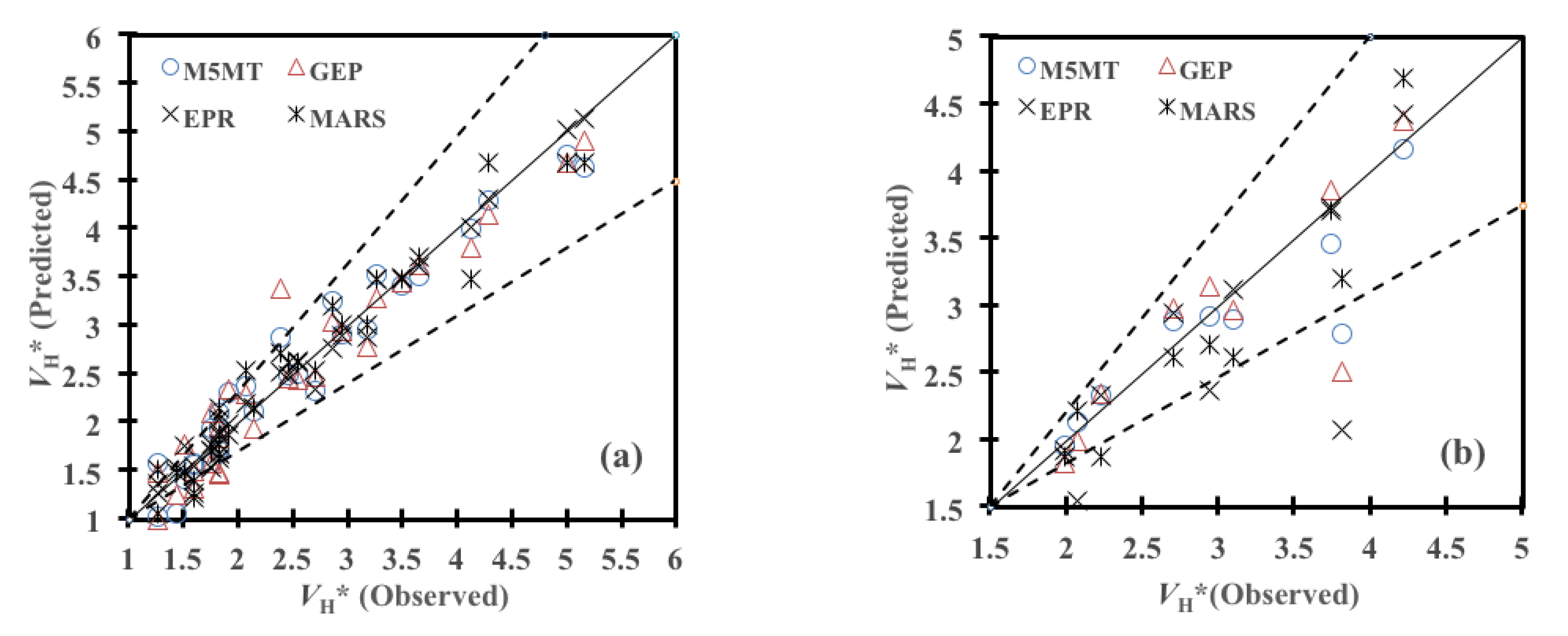
The performance of AI models for the estimation of V H * in training and testing stages is illustrated in Figure 5. In Figure 5, data are fitted to ± 25% error lines. Most values of V H * predicted by the AI models in the training stage were in the range of an acceptable error bound. Similarly, Figure 5b shows well-matched predictions versus experimental observations, though a relatively significant under prediction is seen in the observed value of V H * = 3.8 for M5MT, GEP, and EPR models.
In Table 3, statistical assessments of training and testing results in the prediction of V L * are given. It is inferred that the MARS technique (i.e., Equation (A9)) estimated V L * with the highest level of precision (IOA = 0.9950, SSE = 0.0157, and MAE = 0.0374) in the training phase in comparison with M5MT (IOA = 0.9877, SSE = 0.0387, and MAE = 0.0672), EPR (IOA = 0.9883, SSE = 0.0369, and MAE = 0.0754), and GEP (IOA = 0.9680, SSE = 0.1001, and MAE = 0.1027). SI (0.0504) and ADR (0.9993) obtained by the MARS model were also indicative of its superiority when compared to the other AI models. Table 3 also indicates that M5MT and EPR models had approximately the same performance in the prediction of V L * according to the statistical benchmarks (i.e., IOA, SSE, and SI). Moreover, it can be inferred from the ADR values that all AI models had convincing efficiency; specifically, the MARS model experienced a very marginal under prediction whereas the other AI approaches showed insignificant over predictions. Results of the testing stage demonstrated that the GEP-based formulation (i.e., Equation (A2)) had the best performance (IOA = 0.9911, SSE = 0.0384, and MAE = 0.0544) in the prediction of V L * . M5MT (IOA = 0.9896, SSE = 0.0449, and MAE = 0.0644), and MARS (IOA = 0.9828, SSE = 0.0738, and MAE = 0.0870) stood at the second and third place in terms of precision level, respectively. Ultimately, EPR (i.e., Equation (A5)) provided V L * predictions with the lowest level of accuracy in terms of SSE (0.1322) and MAE (0.0944). SI values confirm an unconvincing performance associated with EPR (SI = 0.1502). ADR values indicated a very marginal under estimation (ADR < 1) for the GEP model.
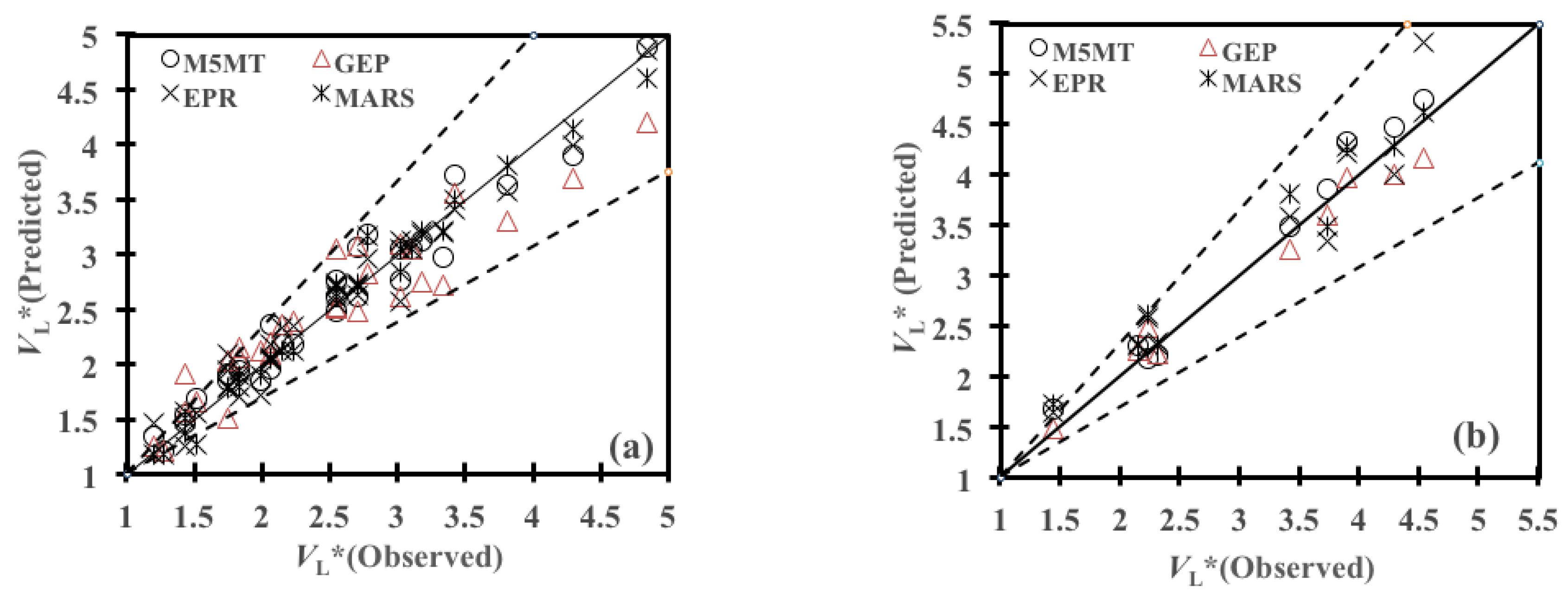
For the sake of qualitative comparisons, Figure 6 illustrates the comparison between predicted and observed values of V L * . In the case of the training stage, Figure 6a shows very compromising efficiency with almost all predictions inside ± 25% error lines. In the case of the testing stage, the EPR model remarkably overpredicted with the observed value of V L * = 4.52 (Figure 6b).
Table 4 shows statistical benchmarks associated with the training and testing phases for prediction of V R * . In the training phase, statistical criteria demonstrated that the EPR-base relationship [Equation (A6)] predicted V R * values with the highest level of accuracy (i.e., IOA = 0.9913, SSE = 0.0345, and MAE = 0.1030) than those obtained by other AI models. Furthermore, SI values given by Table 4 indicate superiority of EPR model over other AI techniques. According to IOA, SSE, and SI criteria, the MARS-based formulation (Equation (B9)) placed second in precision (IOA = 0.9831, SSE = 0.0670, and SI = 0.103), followed by M5MT (IOA = 0.9801, SSE = 0.0788, and SI = 0.1046) and GEP (IOA = 0.976, SSE = 0.0953, and SI = 0.0964). In addition to this, ADR values illustrated that all AI models had compromising performance with values of ADR roughly close to 1. These values are also indicative of very small overpredictions. The assessment of performance for the testing phase indicated that the MARS model (Equation (A9)) had the most accurate prediction in terms of IOA (0.9670), SSE (0.0855), and MAE (0.1086) in comparison to other AI models. Additionally, the value of SI for MARS was indicative of the most successful performance. M5MT with IOA of 0.9435, SSE of 0.1581, and MAE of 0.1356 came in second. The performance of GEP model (Equation (A3)) with IOA = 0.9329 and SSE = 0.1892 was comparatively at the same accuracy level as for EPR (Equation (A6)) (IOA = 0.9356 and SSE = 0.1816). Additionally, MAE and SI values proved similarity of performance between GEP and EPR models. Moreover, MARS model had more significant underprediction (ADR = 0.9578) than GEP (ADR = 1.0020) with very marginal overestimation. ADR analysis also demonstrated that M5MT and EPR provided low underprediction and fairly relative overprediction, respectively.
In terms of illustrative comparisons in training phase, Figure 7a indicated that GEP and MARS techniques underpredicted, with an observed value of V R * = 1.11 .
As it can be seen in Figure 7a, the scatter plot for training phase shows highly prosperous performance with almost all data inside ± 25% error ranges. Relatively important overprediction for M5MT and GEP was seen in Figure 8b at V R * = 2.22 . MARS and GEP techniques underpredicted for V R * = 1.35 , whereas EPR provided significant overprediction.

5.3. Driving Physical Meaning of AI Results

In this section, the physical performance of the AI models is controlled by analyzing 3D scour propagation rates versus e / D and K C values.

5.3.1. Effects of e / D on V H *

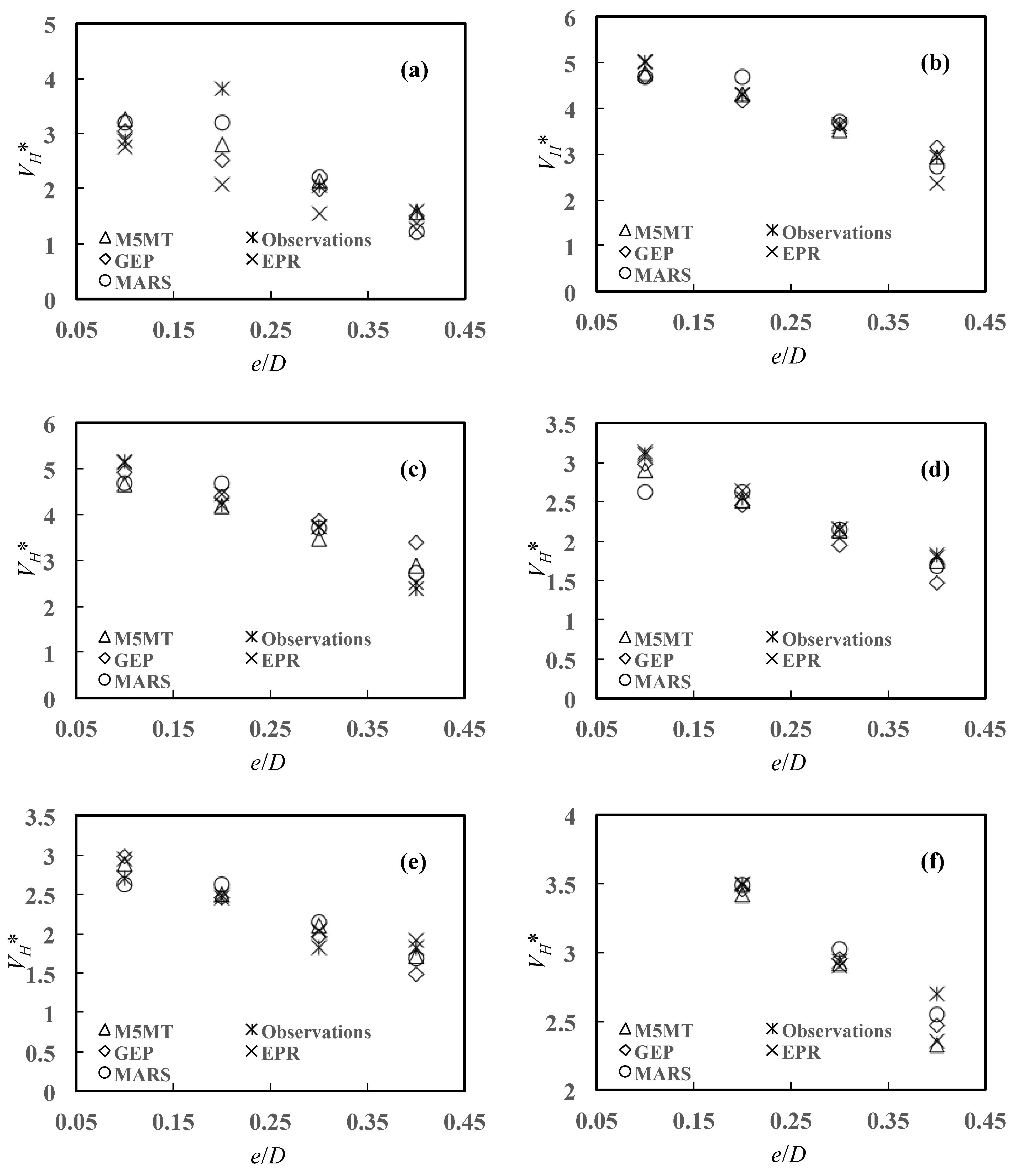
Figure 8 illustrates the variations of V H * as a function of e / D . In fact, this type of variation was assessed for all the considered AI models at various levels of K C and α .
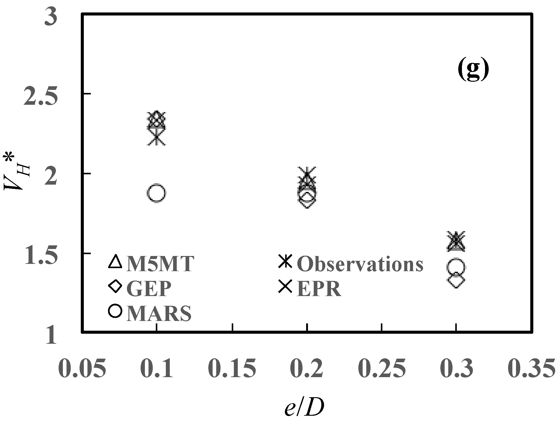
Figure 8a shows that the experimental values of V H * , for KC = 8.7 and α = 0° increase from 2.77 at e/D = 0.1 to 3.81 at e/D = 0.2 and then descend towards 1.51 at e/D = 0.4. This non-monotonic trend is well captured by the MARS model, the results of which are more in harmony with the observations in comparison to the remaining models. All the AI models show underprediction at e/D = 0.2. Quantitatively, the EPR model exhibits significant underprediction with SSE = 0.843 in comparison to GEP (SSE = 0.435), M5MT (SSE = 0.300), and MARS (SSE = 0.161). According to Figure 8b, all the AI models were in satisfying agreement with the observations in the case of KC = 15.8 and α = 0°. Generally, AI models predict a linear downward trend between V H * and e/D, as observed experimentally. Similarly, Figure 8c, which relates to the case of KC = 18.0 and α = 0°, shows an even more pronounced linear decreasing trend between V H * and e/D, quite well captured by all the AI models. EPR had the most satisfying performance (SSE = 0.018), while the GEP model showed a significant overprediction at e/D = 0.4. Figure 8d, which relates to the case KC = 15.8 and α = 30°, exhibiting more alleviated values of V H * when compared to those in Figure 8b. This is due to the higher value of α (equal to 30° here while equal to 0° in Figure 8b); it remains the observed downward trend between V H * and e/D. Moreover, in this case, the considered AI models perform satisfactorily by assessing the effect of the angle α properly, though the MARS model appears more resilient for e/D from 0.1 to 0.2. Moreover, MARS and GEP models indicated marginal underestimations at e/D = 0.1 and 0.4. More specifically, EPR with SSE of 0.003 shows the most compromising efficiency compared to M5MT (SSE = 0.011), GEP (SSE = 0.0468), and MARS (SSE = 0.0631). Figure 8e, which relates to the case KC = 18.0 and α = 30°, clearly shows the effect of the angle α when compared to Figure 8c, while it is less significant in realizing the effect of KC when compared to Figure 8d (on the other hand, KC in Figure 8d is equal to 15.8 and slightly differs from KC = 18.0 in Figure 8e). It is confirmed that V H * decreases with increasing α as well as decreasing with increasing normalized embedment depth e/D (especially for the highest values of KC). AI models are still in harmony with these observed trends. Quantitatively, EPR with an SSE of 0.028 had the most compromising efficiency compared to M5MT (SSE = 0.031), MARS (SSE = 0.040), and GEP (SSE = 0.054). Further effects of the wave angle of attack α on V H * are highlighted in Figure 8g, which relates to the case KC = 15.8 and α = 45°, when Figure 8b,d is considered for comparison. In this analysis, significant underpredictions were found for the MARS model (SSE = 0.054) at e/D = 0.1 and for GEP (SSE = 0.035) and MARS (SSE = 0.054) at e/D = 0.4. For the sake of completeness, Table 5 below shows the performance index SSE for all AI models by varying the normalized embedment depth e/D. Overall, it appears that the M5MT model had the best performance compared to the other AI models, though it is not always quite so straightforward.

5.3.2. Effects of e / D and K C on V R *

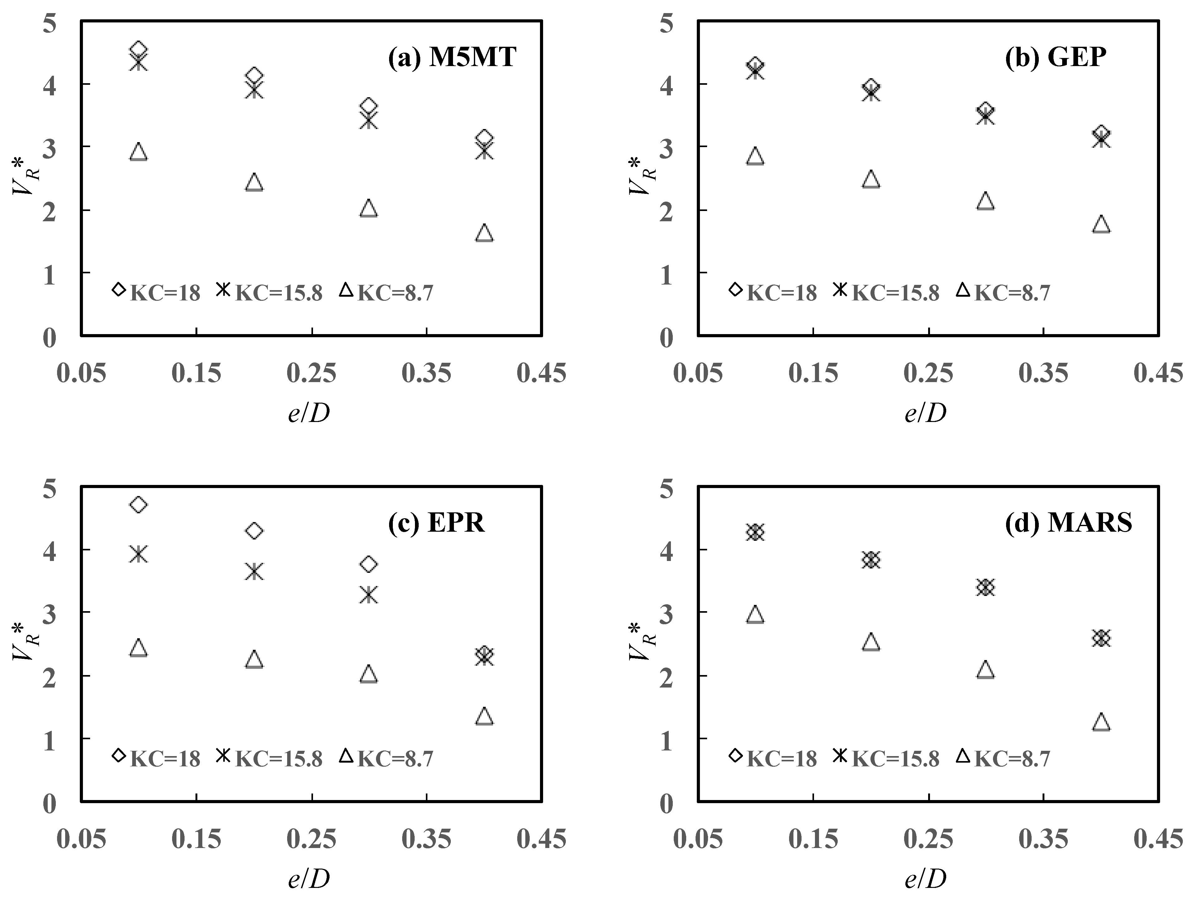
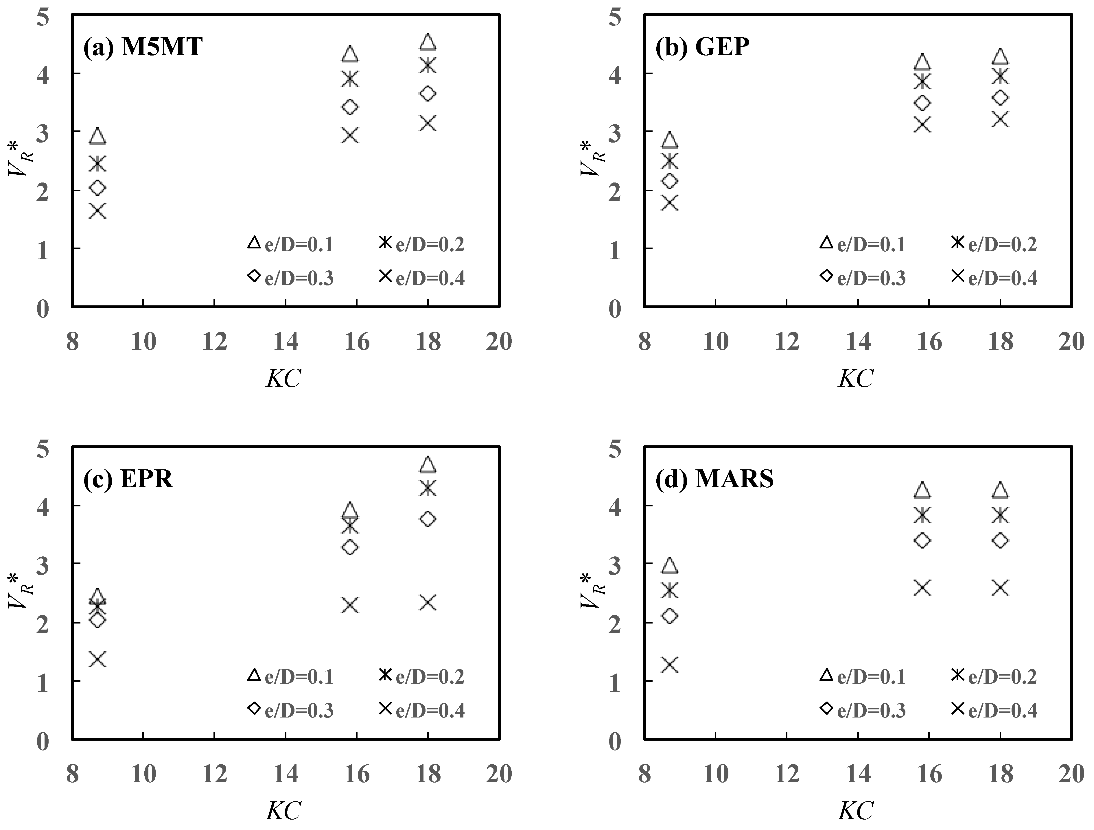
Figure 9a–d shows the variations of V R * against e / D at given values of K C and for α = 0°, according to AI models. All AI models exhibit a downward trend when interpreting the variations of V R * with e / D increasing from 0.1 to 0.4. For example, M5MT simulates that V R * decreases linearly with increasing e / D , as shown in Figure 9a. In addition, for a constant value of e / D , V R * increases with increasing K C , with a tendency towards an asymptotic value. For example, V R * increases sharply from 2.94 for K C = 8.7 to 4.56 for K C = 18, at e / D = 0.1 as shown in Figure 10a. This trend was generally repeated in Figure 9b–d.
Analogously, Figure 10a–d shows the variations of V R * against K C at given values of e / D , according to AI models. All AI models exhibit an upward trend when interpreting the variations of V R * with K C increasing from 8.7 to 18. For example, M5MT simulates that V R * increases from 2.4 for K C = 8.7 to 4.56 for K C = 18, at e / D = 0.2. However, in general, the trend is not linear but approximately asymptotic. In addition, for a constant value of K C , V R * decreases as e / D increasing. For example, V R * values decline from 4.344 for e / D = 0.1 to 2.927 for e / D = 0.4, at K C = 15.8, as shown in Figure 10d.
Moreover, statistical performance of AI techniques for the prediction of V R * with consideration of e / D and K C variations at α = 0° is presented in Table 6. It was found that all the AI techniques had the best performance for better understanding the general pattern of V R * versus e / D at K C = 8.7. For instance, the GEP model indicated the most satisfying efficiency at K C = 8.7 with an SSE of 0.0622 than results predicted at K C = 15.8 (SSE = 0.2602) and K C = 18 (SSE = 0.0827). For K C = 8.7, EPR was found more compromisingly for the assessment of V R * with SSE = 0.0168 in comparison with M5MT (SSE = 0.0388), MARS (SSE = 0.0483), and GEP (SSE = 0.0622). In the case of K C = 15.8, EPR had the most successful efficiency while for K C = 18, the M5MT technique stood at the highest level of accuracy for simulation of V R * variations versus e / D ratios. In Table 6, it was inferred that AI models indicated the best performance to perceive variations of V R * versus K C values for different e / D ratios. MARS (SSE = 0.0544), M5MT (SSE = 0.0244), and EPR (SSE = 0.0035) had the most accurate efficiency at e / D = 0.3 while for e / D = 0.1, the GEP technique had the most prosperous performance (SSE = 0.0349). GEP showed variations of V R * versus at e / D = 0.1, with the highest level of accuracy (SSE = 0.0349) whereas for e / D = 0.2, EPR was determined as the most precise model. On the other hand, EPR (SSE = 0.0035) and MARS (SSE = 0.0920) stood at the highest level of accuracy at e / D = 0.3 and e / D = 0.4, respectively.

5.3.3. Effects of e / D and K C on V L *

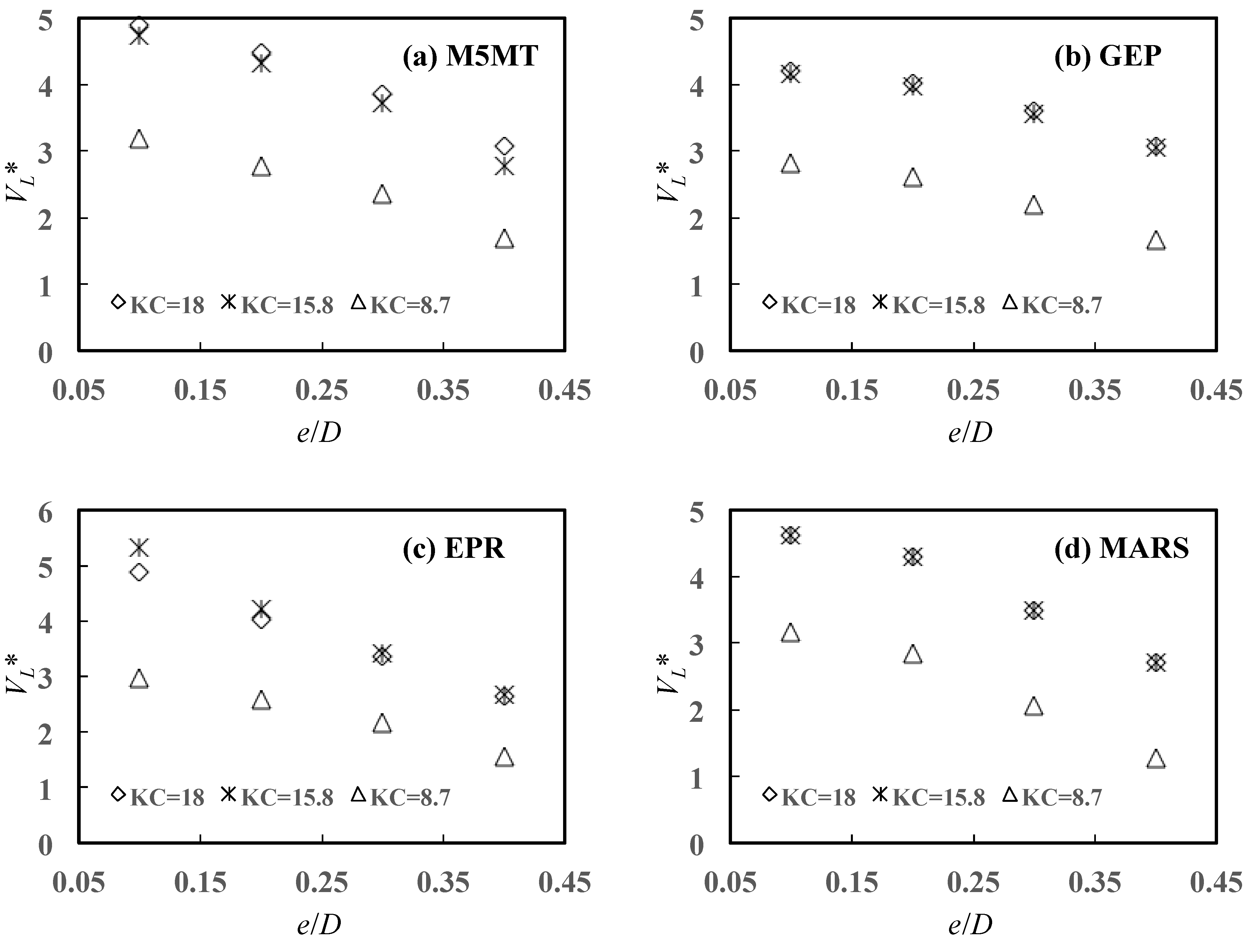
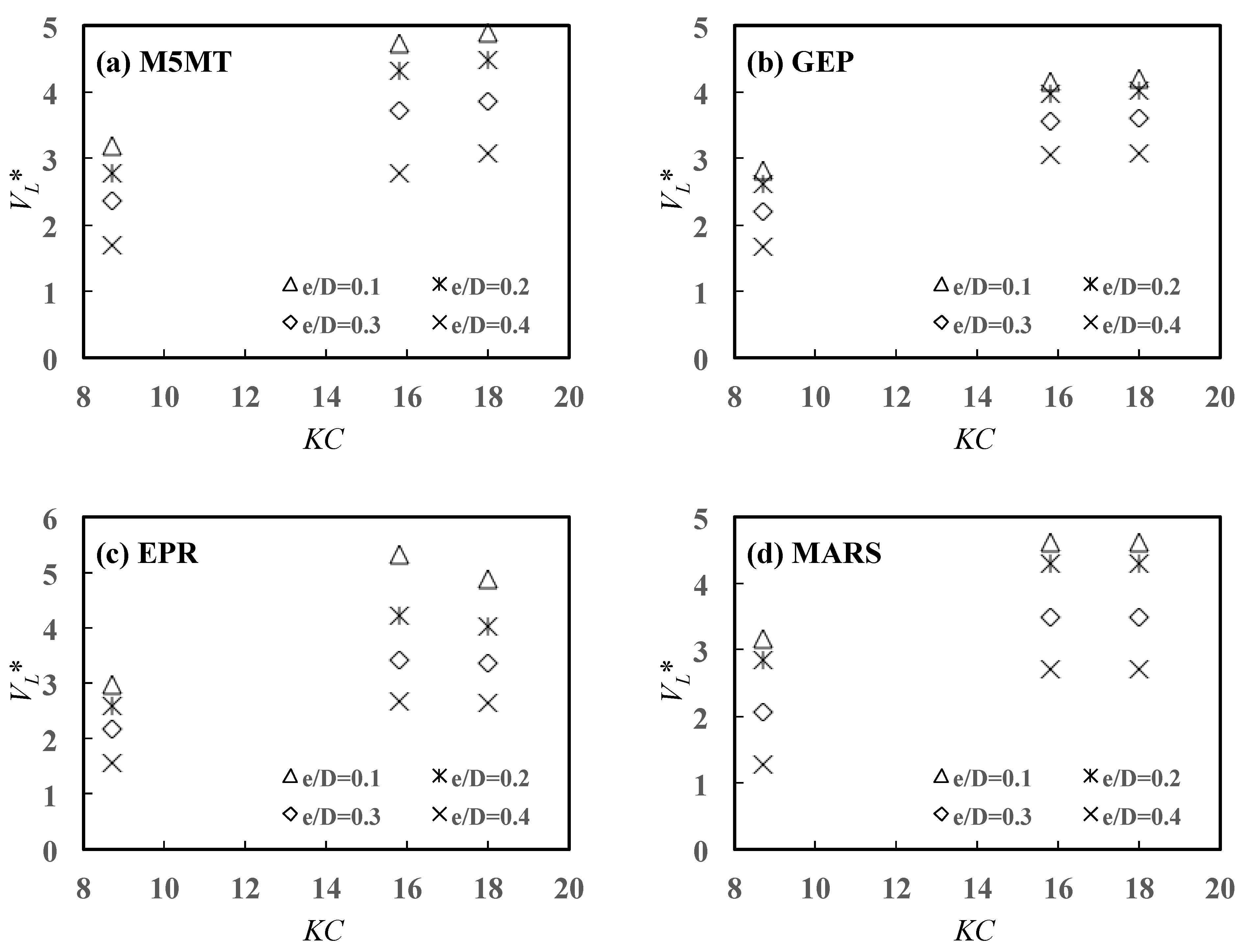
Figure 11a–d shows the variations of V L * against e / D at given values of K C , and for α = 0°, according to AI models. All AI models exhibit a downward trend when interpreting the variations of V L * with e / D increasing from 0.1 to 0.4. For example, M5MT simulates that V L * decreases linearly with increasing e / D , as shown in Figure 11a. In addition, for a constant value of e / D , V L * increases with increasing K C , with a tendency towards an asymptotic value. For example, V L * increases sharply from 2.776 for K C = 8.7 to 4.482 for K C = 18, at e / D = 0.2.
Analogously, Figure 12a–d shows the variations of V L * against K C at given values of e / D , according to AI models. All AI models exhibit an upward trend when interpreting the variations of V L * with K C increasing from 8.7 to 18. For example, GEP simulates that V L * increases from 2.83 for K C = 8.7 to 4.207 for K C = 18, at e / D = 0.1. However, in general, the trend is not linear but approximately asymptotic. In addition, for a constant value of K C , V L * decreases with e / D increasing. For example, V L * plummets from 4.168 for e / D = 0.1 to 3.047 for e / D = 0.4, at K C = 15.8, as shown in Figure 12b.
According to Table 7, the GEP model had the best performance (SSE = 0.0502) at K C = 8.7 while all other AI models indicated the most accurate prediction of V L * values for K C = 18. The EPR technique predicted variations of V L * versus e / D with highly satisfying performance at K C = 15.8 (SSE = 0.0494) and K C = 18 (SSE = 0.0272). Table 7 also indicates that M5MT (SSE = 0.0658), EPR (SSE = 0.0207), and GEP (SSE = 0.0188) had the most favorable performance at e / D = 0.3 while MARS (SSE = 0.00633) stood at the highest level of efficiency at e / D = 0.4. EPR model indicated more successful efficiency for e / D = 0.1 (SSE = 0.0720) and e / D = 0.2 (SSE = 0.0617) than the remaining AI models. What is more, GEP raised the most well-matched predictions for the variations of V L * versus K C with SSE = 0.0188 at e / D = 0.2, while EPR had the best performance (SSE = 0.00633) at e / D = 0.4.

6. Conclusions

This study aimed to explore 3D scouring patterns around subsea pipelines under wave-only conditions. To this purpose, the experimental work by Cheng et al. [9] was considered. Experimental data were collected in a wave flume 50 m long, 4 m wide, and 2.5 m deep. A total of 60 wave-only tests were considered, though some of these tests (i.e., 22 tests) have proved to be of no use. An almost uniform siliceous sand with d 50 equal to 0.37 mm and specific gravity of 2.70 was used for the mobile bed. Experiments were conducted under live-bed conditions with the Shields’ parameter θ w ranging from 0.18 to 0.30, the Keulegan–Carpenter number K C from 8.7 to 18.0, the initial pipeline embedment depth, e , from 0.1 D to 0.5 D , and the flow incident angle, α , relative to the pipeline varying from 0° to 45°. Four robust data-driven models were applied to predict the 3D scour propagation around undersea pipelines, namely Gene-Expression Programming (GEP), Evolutionary Polynomial Regression (EPR), Multivariate Adaptive Regression Spline (MARS), and M5 Model Tree (M5MT). Generally, the following conclusions can be drawn from the current investigation:
  • The considered predictive methodologies indicated two main potentialities: (i) Providing non-linear regression equations with a high degree of complexity (as naturally seen in the scouring process around submarine pipelines) when developed by a limit volume of datasets; (ii) selecting the effective variables (i.e., e / D , K C , α , θ w ) on the scour rates estimation under a full automated manner.
  • All AI models applied in this study provided explicit relationships with satisfying performance for the prediction of 3D scour rates. However, the performance indices in the training and testing phases overall revealed that the MARS technique is most the eligible one. Therefore, the scour Equations (A7)–(A9), given in Appendix B, associated with the Basis Functions (BFs) explicitly stated in Table A3, are recommended in the prediction of V H * , V L * , and V R * , respectively.
  • The physical consistency of the AI models was controlled by analyzing 3D scour propagation rates versus the normalized embedment depth e / D , the flow incident angle α , and Keulegan–Carpenter number K C . It was confirmed that scour propagation rates decrease with increasing e / D , decrease with increasing the angle of attack α , and increase with K C number. Conversely, it was ascertained the Shields’ parameter does not control, at least significantly, the scour rate propagation at the right- and left-hand pipeline shoulders.
  • A comparison with the conventional approach by [9] for the prediction of V H * would prove the superiority of the proposed scour equations. For example, by applying Equation (8) in [9], the performance index IOA is 0.842, significantly lower than the values of IOA for all the considered AI techniques (i.e., 0.9670 for MARS, 0.9435 for M5MT, 0.9356 for EPR, and 0.9329 for GEP).

Author Contributions

Conceptualization, M.N. and G.O.; methodology, M.N.; software, M.N.; validation, M.N. and G.O.; formal analysis, M.N. and G.O.; investigation, M.N. and G.O.; data curation, M.N. and G.O.; writing—original draft preparation, M.N. and G.O.; writing—review and editing, M.N. and G.O.; visualization, M.N. and G.O.; supervision, M.N. and G.O. All authors have read and agreed to the published version of the manuscript.

Funding

This research received no external funding.

Conflicts of Interest

The authors declare no conflict of interest.

List of Notations and Acronyms

Notations
a i constant coefficient in M5MT model
cnumber of elements in input vectors in EPR model
Dpipeline diameter
d 50 median grain size of the seabed sediment
epipeline embedment depth
ESexponent range in EPR model
g acceleration due to gravity
K C Kelugan -Carpenter number
m maximum number of mathematical terms in EPR model
N number of experimental observations
O number of input variables in MARS model
Q number of Basis Functions in MARS model
R e w pipeline Reynolds number
Twave period
U w wave orbital velocity at the seabed
V H scour propagation velocity along the longitudinal (axial) direction of the pipeline
V L scour propagation velocity at the left-hand shoulder of the pipeline
V R scour propagation velocity at the right-hand shoulder of the pipeline
V E s t * computed scour rate value
V H , L , R * dimensionless scour propagation velocity
V O b s * observed scour rate value
V E s t * ¯ average value for computed scour rate values
V O b s * ¯ average value for observed scour rate values
x i i-th input variable in MARS model
Xvector of input variables in MARS model
zspecific function in EPR model
α flow incident angle to the pipeline (or angle of attack)
ϕ angle of repose of the seabed sediment
Γoutput vector in EPR model
η i i-th input vector in EPR model
θ w Shields’ parameter
μ dynamic viscosity of water
i i-th non-dimensional parameter
ρ density of water
ρ s density of sediment
ωset of weighting coefficients in MARS model
ω i i-th weighting coefficient in MARS model
ω 0 constant coefficient in MARS model
Ωapproximation function in MARS model
ξ 0 bias term in EPR model
ξ j j-th coefficient in EPR model
Acronyms
ADRAverage Discrepancy Ratio
AIArtificial Intelligence
ANFISAdaptive Neuro-Fuzzy Inference System
ANNArtificial Neural Network
BPBack Propagation
CARTClassification and Regression Tree
CBOColliding Bodies’ Optimization
CWClear-Water regime
EPREvolutionary Polynomial Regression
GEPGene-Expression Programming
GMDHGroup Method of Data Handling
GPGenetic Programming
IOAIndex Of Agreement
LBLive-Bed regime
LGPLinear Genetic Programming
MAEMean Absolute Error
MARSMultivariate Adaptive Regression Splines
MNLRMultivariate Non-Linear Regression
MSEMean Square Error
cMTModel Tree
PSOParticle Swarm Optimization
SIScatter Index
SSESum of Squared Errors
SVMSupport Vector Machine
WAWale Algorithm

Appendix A. Experiments by Cheng et al. (2014): Test Conditions and Main Results

In this Appendix the tests of Cheng et al. [9] are summarized in terms of test conditions and main results. Only the tests considered in this study are given below (Table A1). It should be noted that H is the wave height.
Table A1. Tests of [9]: main characteristics and results under wave-only conditions.
Test# α e / D H T U w K C θ w V H V L V R
[-][°][-][m][s][m/s][-][-][mm/s][mm/s][mm/s]
w15t15e10.10.131.50.298.70.183.53.63.4
w15t15e20.20.131.50.298.70.183.84.82.8
w15t15e30.30.131.50.298.70.182.62.62.6
w15t15e40.40.131.50.298.70.181.92.01.8
w16t18e10.10.171.80.4415.80.305.76.35.1
w16t18e20.20.171.80.4415.80.304.95.44.4
w16t18e30.30.171.80.4415.80.304.34.64.0
w16t18e40.40.171.80.4415.80.303.23.72.8
w16t20e10.10.152.00.4518.00.296.16.55.7
w16t20e20.20.152.00.4518.00.295.45.35.5
w16t20e30.30.152.00.4518.00.294.74.74.7
w16t20e40.40.152.00.4518.00.293.43.03.7
a15w15t15e315°0.30.131.50.298.70.182.21.62.7
a15w15t15e415°0.40.131.50.298.70.181.51.61.5
a15w16t18e115°0.10.171.80.4415.80.305.45.25.6
a15w16t18e215°0.20.171.80.4415.80.304.34.14.5
a15w16t18e315°0.30.171.80.4415.80.304.24.04.4
a15w16t18e415°0.40.171.80.4415.80.302.82.63.1
a15w16t20e215°0.20.152.00.4518.00.294.84.45.2
a15w16t20e315°0.30.152.00.4518.00.294.03.74.3
a15w16t20e415°0.40.152.00.4518.00.293.23.43.0
a30w15t15e130°0.10.131.50.298.70.182.62.23.0
a30w15t15e230°0.20.131.50.298.70.181.82.21.4
a30w16t18e130°0.10.171.80.4415.80.303.93.94.0
a30w16t18e230°0.20.171.80.4415.80.303.43.23.6
a30w16t18e330°0.30.171.80.4415.80.302.92.73.1
a30w16t18e430°0.40.171.80.4415.80.302.52.32.6
a30w16t20e130°0.10.152.00.4518.00.293.83.44.1
a30w16t20e230°0.20.152.00.4518.00.293.23.13.4
a30w16t20e330°0.30.152.00.4518.00.292.72.33.1
a30w16t20e430°0.40.152.00.4518.00.292.32.32.3
a45w15t15e145°0.10.131.50.298.70.181.81.91.7
a45w15t15e245°0.20.131.50.298.70.181.61.81.4
a45w16t18e145°0.10.171.80.4415.80.302.72.82.7
a45w16t18e245°0.20.171.80.4415.80.302.22.51.9
a45w16t18e345°0.30.171.80.4415.80.301.82.01.6
a45w16t20e145°0.10.152.00.4518.00.292.82.43.1
a45w16t20e245°0.20.152.00.4518.00.292.32.32.3

Appendix B. Implementation of the Intelligent Computing Methods: Tables and Equations

  • GEP-derived equations
The parameters characterizing the GEP method for 3D-scour rate predictions are made explicit in Table A2.
Table A2. Parameters of the GEP model for 3D-scour rate predictions.
ParametersDescription of ParametersSetting of Parameters
P1Function set+,−,·,/, Power (x2), min(x1, x2), (1−x), ln(x), average(x1, x2), arctan(x), tanh(x)
P2Linking functionAddition
P3Mutation rate0.003
P4Inversion rate0.00546
P5One-point and two-point recombination rates0.00277
P6Gene recombination rate 0.00277
P7Permutation0.00546
P8Maximum tree depth6
P9Number of genes3
P10Number of chromosomes30
P11Best fitness values773.67 ( V H * ), 763.76 ( V R * ), 761.35 ( V L * )
GEP models have been developed via GeneXproTools5 platform. During their development, the values of best-fit function were 1687, 1123, and 1322 for the estimation of V H * , V R * , and V L * , respectively. The best formulations were the following:
V H * = t a n h ( a r c t a n   ( l n   ( min ( 3.8810 + K C , ( 1 e D ) 2 ) ) ) ) + [ K C e D + s i n α + ( 2.3133 e D ) · ( 1 e D ) ] + m i n [ t a n h ( ( θ w 1 + s i n α ) ) · ( 4.1825 + K C 2 ) , 3.9524 ( 1 + s i n α ) 2   ]
V L * = [ e D + s i n α + 3.5804 s i n α 2 ] + { a r c t a n   [ 1 0.5 · ( 2 + s i n α e D ) + m i n ( 8.9196 K C , θ w 1 s i n α ) 2 ] } 2 + [ 1 { t a n h ( 1 + e D + s i n α ( 1 e D ) 2 ) } 4 ]
V R * = [ 1 e D + θ w ( 1 + s i n α ) 2 ] · ( s i n α e D ) 1 3 + { t a n h [ a r c t a n ( K C 3.836 2 ) ] + 1 e D } 2 + 1 [ t a n h ( 1 e D ) 2 K C + e D ] · θ w 2  
  • EPR-derived equations
EPR models have been developed by EPR MOGA-XL software. The best formulations for the estimation of V H * , V R * , and V L * were the following:
V H * = 0.3235 · ( K C ) 0.5 + 0.02161 · ( 1 e D ) 0.5 K C 0.5 θ w 2 · l n [ K C 2 · θ w 2 ( 1 e D ) 2 · ( 1 + s i n α ) 0.5 ] + 0.00278 · ( 1 + s i n α ) 0.5 ( 1 e D ) 0.5 K C 0.5 θ w 0.5 · l n [ ( 1 e D ) 0.5 · θ w 0.5 ( 1 + s i n α ) ] + 0.01438 · ( 1 + s i n α ) 2 K C 0.5 θ w · l n [ ( 1 e D ) 0.5 · ( 1 + s i n α ) 2 · θ w 2 K C 0.5 ]
V L * = 0.01157 · L n [ θ w K C 2 · ( 1 + s i n α ) ] + 0.001464 · l n [ ( 1 e D ) · ( 1 + s i n α ) · θ w 0.5 ] + 0.3205 · ( 1 e D ) + 0.01153 · ( 1 e D ) 2 · θ w 2 K C · l n [ ( 1 e D ) 2 · θ w 2 · K C 2 ( 1 + s i n α ) 0.5 ] + 0.4768 · ( 1 + s i n α ) · l n [ 1 ( 1 + s i n α ) 1.5 ]
V R * = 0.000671 · l n [ θ w K C 2 · ( 1 + s i n α ) 1.5 ] + 0.3438 · K C 0.5 · θ w + 0.01371 · ( 1 e D ) 2 · K C θ w · l n [ K C 1.5 ( 1 e D ) · ( 1 + s i n α ) 1.5 · θ w 2 ] + 0.57711 · ( 1 + s i n α ) 0.5 ( 1 e D ) 0.5   · l n [ ( 1 e D ) 0.5 ( 1 + s i n α ) 2 ] + 0.02773 · ( 1 + s i n α ) 2 ( 1 e D ) 2 · l n [ ( 1 e D ) 2 · ( 1 + s i n α ) 2 θ w 0.5 ]
  • MARS-derived equations
The formulations for the basis functions (BFs) and their weighting coefficients associated with the estimation of 3D- scour rates are listed in Table A3.
Table A3. Explored basis functions (BFs) in MARS models for 3D-scour rate predictions.
BFs   for   V H * Prediction
BF1 m a x { 0 ,   0.29 θ w }
BF2 m a x { 0 ,   0.29 θ w } · m a x { 0 , [ ( 1 + s i n α ) 1.2587 ] }
BF3 m a x { 0 ,   [ 0.8 ( 1 e / D ) ] }
BF4 m a x { 0 , [ 0.8 ( 1 e / D ) ] } · m a x { 0 , [ 1.2587 ( 1 + s i n α ) ] }
BF5 m a x { 0 , [ ( 1 + s i n α ) 1.258 ] }
BF6 m a x { 0 , [ 1.2587 ( 1 + s i n α ) ] }
BFs   for   V L * Prediction
BF1 m a x { 0 ,   [ ( 1 + s i n α ) 1.258 ] }
BF2 m a x { 0 ,   [ 1.258 ( 1 + s i n α ) ] }
BF3 m a x { 0 ,   [ ( 1 e / D ) 0.8 ] }
BF4 m a x { 0 ,   [ 0.8 ( 1 e / D ) ] }
BF5 m a x { 0 ,   15.8 K C }
BF6 m a x { 0 ,   15.8 K C } · m a x { 0 , [ ( 1 + s i n α ) 1.258 ] }
BF7 m a x { 0 , [ 0.8 ( 1 e / D ) ] } · m a x { 0 , [ 1.2587 ( 1 + s i n α ) ] }
BFs   for   V R * Prediction
BF1 m a x { 0 ,   15.8 K C }
BF2 m a x { 0 ,   [ ( 1 e / D ) 0.7 ] }
BF3 m a x { 0 ,   [ 0.7 ( 1 e / D ) ] }
BF4 m a x { 0 ,   [ ( 1 + s i n α ) 1.258 ] }
MARS models have been developed by MATLAB2015 software. The best formulations for the estimation of V H * ,   V R * , and V L * were the following:
V H * = 3.4903 13.568 · B F 1 + 22.259 · B F 2 4.7028 · B F 3 20.026 · B F 4 3.5962 · B F 5 + 4.6579 · B F 6
V L * = 3.8165 4.4937 · B F 1 + 1.8162 · B F 2 + 3.2772 · B F 3 4.1566 · B F 4 0.20284 · B F 5 0.2084 · B F 6 7.4663 · B F 7
V R * = 3.3939 0.18259 · B F 1 + 4.3799 · B F 2 8.1073 · B F 3 4.2723 · B F 4
  • M5MT-derived equations
Table A4 and Table A5 summarize, respectively, M5 rules and associated linear equation returned by Model Tree for the prediction of V H * . 12 rules were provided and, additionally, all the four input variables were used as splitting parameters.
Table A4. List of explored rules returned by M5MT model to predict V H * .
If 1+ sinα <= 1.379:
|   If 1  e/D <= 0.75:
|   |   If KC <= 12.25: LM#1
|   |   If KC > 12.25:
|   |   |   If 1  e/D <= 0.65: LM#2
|   |   |   If 1  e/D > 0.65: LM#3
|   If 1  e/D > 0.75:
|   |   If 1+ sinα <= 1.129:
|   |   |   If θw <= 0.295: LM#4
|   |   |   If θw > 0.295: LM#5
|   |   If 1+ sinα > 1.129: LM#6
If 1+ sinα > 1.379:
|   If KC <= 12.25:
|   |   If 1+ sinα <= 1.603: LM#7
|   |   If 1+ sinα > 1.603: LM#8
|   If KC > 12.25:
|   |   If 1-e/D <= 0.65: LM#9
|   |   If 1- e/D > 0.65:
|   |   |   If 1+ sinα <= 1.603:
|   |   |   |   If 1  e/D <= 0.75: LM#10
|   |   |   |   If 1- e/D > 0.75: LM#11
|   |   |   If 1+ sinα > 1.603: LM#12
Table A5. Linear equations obtained by M5MT model to predict V H * .
Linear Equations by M5MT Model
#1 V H * = 1.5478 2.1346 · ( 1 + s i n α ) + 5.5576 · ( 1 e D ) + 0.0246 · K C + 9.5079 · θ w
#2 V H * = 1.602 2.1346 · ( 1 + s i n α ) + 5.811 · ( 1 e D ) + 0.0211 · K C + 9.5079 · θ w
#3 V H * = 1.602 2.1346 · ( 1 + s i n α ) + 5.811 · ( 1 e D ) + 0.0211 · K C + 9.5079 · θ w
#4 V H * = 0.4133 2.793 · ( 1 + s i n α ) + 4.6905 · ( 1 e D ) + 12.512 · θ w
#5 V H * = 0.4133 2.793 · ( 1 + s i n α ) + 4.6905 · ( 1 e D ) + 12.5124 · θ w
#6 V H * = 0.2965 2.8258 · ( 1 + s i n α ) + 4.6905 · ( 1 e D ) + 12.5124 · θ w
#7 V H * = 1.2191 2.4643 · ( 1 + s i n α ) + 3.5315 · ( 1 e D ) + 0.0209 · K C + 5.8612 · θ w
#8 V H * = 1.2191 2.4643 · ( 1 + s i n α ) + 3.5315 · ( 1 e D ) + 0.0209 · K C + 5.8612 · θ w
#9 V H * = 1.3753 2.6322 · ( 1 + s i n α ) + 3.8196 · ( 1 e D ) + 0.0166 · K C + 5.8612 · θ w
#10 V H * = 1.3642 2.6582 · ( 1 + s i n α ) + 3.8972 · ( 1 e D ) + 0.0166 · K C + 5.8612 · θ w
#11 V H * = 1.3649 2.6582 · ( 1 + s i n α ) + 3.8972 · ( 1 e D ) + 0.0166 · K C + 5.8612 · θ w
#12 V H * = 1.4057 2.6653 · ( 1 + s i n α ) + 3.8509 · ( 1 e D ) + 0.0166 · K C + 5.8612 · θ w
Table A6 and Table A7 show that in the case of V L * estimation, 12 rules were obtained from M5 analysis with the splitting of the parameters 1 + sin α , 1 e / D , and K C .
Table A6. List of explored rules returned by M5MT model to predict V L * .
Rule#1
IF 1+sinα <= 1.603, 1  e/D <= 0.65, KC > 12.25, 1+ sinα <= 1.379
THEN LM#1
Rule#2
IF 1+ sinα <= 1.603, 1  e/D > 0.65, KC <= 12.25, 1+ sinα <= 1.129
THEN LM#2
Rule#3
IF KC > 12.25, 1+ sinα <= 1.379, 1  e/D <= 0.75
THEN LM#3
Rule#4
IF KC > 12.25, 1+ sinα <= 1.379
THEN LM#4
Rule#5
IF KC > 12.25, 1+ sinα > 1.603, 1  e/D <= 0.85
THEN LM#5
Rule#6
IF KC <= 12.25, 1+ sinα <= 1.603, 1  e/D <= 0.65
THEN LM#6
Rule#7
IF KC <= 12.25, 1+ sinα <= 1.603
THEN LM#7
Rule#8
IF 1+ sinα <= 1.603, 1  e/D <= 0.7
THEN LM#8
Rule#9
IF KC <= 12.25
THEN LM#9
Rule#10
IF 1+ sinα <= 1.603, 1  e/D <= 0.85
THEN LM#10
Rule#11
IF 1+ sinα <= 1.603
THEN LM#11 = 3.7233×(1+ sinα)+8.642
Otherwise
Rule#12 LM#12
Table A7. Linear equations obtained by M5MT model to predict V L * .
Linear Equations by M5MT Model
#1 V L * = 0.4207 2.2586 · ( 1 + s i n α ) + 4.0342 · ( 1 e D ) + 0.1384 · K C
#2 V L * = 0.71 2.5502 · ( 1 + s i n α ) + 4.1387 · ( 1 e D ) + 0.1501 · K C
#3 V L * = 2.2943 2.8549 · ( 1 + s i n α ) + 4.6573 · ( 1 e D ) + 0.0646 · K C
#4 V L * = 3.1812 3.2497 · ( 1 + s i n α ) + 4.1348 · ( 1 e D ) + 0.0691 · K C
#5 V L * = 2.1734 2.5643 · ( 1 + s i n α ) + 3.8075 · ( 1 e D ) + 0.0639 · K C
#6 V L * = 0.6837 1.3108 · ( 1 + s i n α ) + 2.6787 · ( 1 e D ) + 0.0823 · K C
#7 V L * = 1.9259 2.0976 · ( 1 + s i n α ) + 2.7366 · ( 1 e D ) + 0.0829 · K C
#8 V L * = 3.6165 3.1164 · ( 1 + s i n α ) + 3.6362 · ( 1 e D ) + 0.046 · K C
#9 V L * = 4.4871 3.7599 · ( 1 + s i n α ) + 3.2793 · ( 1 e D ) + 0.0609 · K C
#10 V L * = 4.2091 3.3313 · ( 1 + s i n α ) + 4.2603 · ( 1 e D )
#11 V L * = 8.462 3.7233 · ( 1 + s i n α )
#12 V L * = 2.1843
13 rules in terms of linear regression equations were extracted from M5 to predict V R * , as indicated in Table A8 and Table A9.
Table A8. List of explored rules returned by M5MT model to predict V R * .
If KC <= 12.25:
|   If 1  e/D <= 0.85:
|   |   If 1+ sinα <= 1.379: LM#1
|   |   If 1+ sinα > 1.379: LM#2
|   If 1  e/D > 0.85: LM#3
If KC > 12.25:
|   If 1+ sinα <= 1.379:
|   |   If 1  e/D <= 0.75:
|   |   |   If 1  e/D <= 0.65: LM#4
|   |   |   If 1  e/D > 0.65:
|   |   |   |   If 1+ sinα <= 1.129: LM#5
|   |   |   |   If 1+ sinα > 1.129: LM#6
|   |   If 1  e/D > 0.75:
|   |   |   If KC <=16.9: LM#7
|   |   |   If KC > 16.9: LM#8
|   If 1+ sinα > 1.379:
|   |   If 1+ sinα <= 1.603:
|   |   |   If 1  e/D <= 0.85:
|   |   |   |   If 1  e/D <= 0.75: LM#9
|   |   |   |   If 1  e/D > 0.75: LM#10
|   |   |   If 1  e/D > 0.85: LM#11
|   |   If 1+ sinα > 1.603:
|   |   |   If 1  e/D <= 0.85: LM#12
|   |   |   If 1  e/D > 0.85: LM#13
Table A9. Linear equations obtained by M5MT model to predict V R * .
Linear Equations by M5MT Model
#1 V R * = 0.3424 2.154 · ( 1 + s i n α ) + 4.0823 · ( 1 e D ) + 0.1151 · K C
#2 V R * = 0.3424 2.1582 · ( 1 + s i n α ) + 4.0823 · ( 1 e D ) + 0.1151 · K C
#3 V R * = 0.2434 2.1481 · ( 1 + s i n α ) + 4.2686 · ( 1 e D ) + 0.1151 · K C
#4 V R * = 0.4536 2.0057 · ( 1 + s i n α ) + 4.9602 · ( 1 e D ) + 0.0951 · K C
#5 V R * = 0.5106 2.0057 · ( 1 + s i n α ) + 4.8913 · ( 1 e D ) + 0.0951 · K C
#6 V R * = 0.5106 2.0057 · ( 1 + s i n α ) + 4.8913 · ( 1 e D ) + 0.0951 · K C
#7 V R * = 0.902 2.0057 · ( 1 + s i n α ) + 4.36 · ( 1 e D ) + 0.0964 · K C
#8 V R * = 0.9056 2.0057 · ( 1 + s i n α ) + 4.36 · ( 1 e D ) + 0.0964 · K C
#9 V R * = 2.4404 2.8991 · ( 1 + s i n α ) + 4.341 · ( 1 e D ) + 0.0685 · K C
#10 V R * = 2.4387 2.8991 · ( 1 + s i n α ) + 4.3454 · ( 1 e D ) + 0.0685 · K C
#11 V R * = 1.3649 2.8991 · ( 1 + s i n α ) + 4.3111 · ( 1 e D ) + 0.0685 · K C
#12 V R * = 2.5596 3.0402 · ( 1 + s i n α ) + 4.3839 · ( 1 e D ) + 0.0685 · K C
#13 V R * = 2.5652 3.0402 · ( 1 + s i n α ) + 4.3839 · ( 1 e D ) + 0.0685 · K C

References

  1. Xie, L.; Zhu, Y. Scour protection of underwater pipelines. J. Civ. Eng. Constr. 2018, 7, 171–177. [Google Scholar] [CrossRef] [Green Version]
  2. Sumer, B.M.; Fredsøe, J. The Mechanics of Scour in the Marine Environment; Advanced Series on Ocean Engineering; World Scientific Publishing: Singapore, 2002; Volume 17. [Google Scholar]
  3. Cevik, E.; Yüksel, Y. Scour under submarine pipelines in waves in shoaling conditions. J. Waterw. Port Coast. Ocean Eng. 1999, 125, 9–19. [Google Scholar] [CrossRef]
  4. Hansen, E.A. Scour below pipelines and cables: A simple model. In Proceedings of the 11th Offshore Mechanics and Arctic Engineering Conference, ASME, Calgary, AB, Canada, 7–12 June 1992; Volume V-A, pp. 133–138. [Google Scholar]
  5. Kumar, A.V.; Neelamani, S.; Rao, S.N. Wave pressures and uplift forces on and scour around submarine pipeline in clayey soil. Ocean Eng. 2003, 30, 271–295. [Google Scholar] [CrossRef]
  6. Cheng, L.; Yeow, K.; Zhang, Z.; Teng, B. Three-dimensional scour below offshore pipelines in steady currents. Coast. Eng. 2009, 56, 577–590. [Google Scholar] [CrossRef]
  7. Yang, L.; Shi, B.; Guo, Y.; Wen, X. Calculation and experiment on scour depth for submarine pipeline with a spoiler. Ocean Eng. 2012, 55, 191–198. [Google Scholar] [CrossRef]
  8. Wu, Y.; Chiew, Y.-M. Three-dimensional scour at submarine pipelines. J. Hydraul. Eng. 2012, 138, 788–795. [Google Scholar] [CrossRef]
  9. Cheng, L.; Yeow, K.; Zang, Z.; Li, F. 3D scour below pipelines under waves and combined waves and currents. Coast. Eng. 2014, 83, 137–149. [Google Scholar] [CrossRef] [Green Version]
  10. Yang, L.; Shi, B.; Guo, Y.; Zhang, L.; Zhang, J.; Han, Y. Scour protection of submarine pipelines using rubber plates underneath the pipes. Ocean Eng. 2014, 84, 176–182. [Google Scholar] [CrossRef] [Green Version]
  11. Yusoff, M.A.M.; Azamathulla, H.M.; Ghani, A.A. Time variations of scour below submerged skewed pipelines. IOP Conf. Series: Mater. Sci. Eng. 2016, 136, 012071. [Google Scholar] [CrossRef] [Green Version]
  12. Dogan, M.; Aksoy, A.O.; Arisoy, Y.; Guney, M.S.; Abdi, V. Experimental investigation of the equilibrium scour depth below submerged pipes both in live-bed and clear-water regimes under the wave effect. Appl. Ocean Res. 2018, 80, 49–56. [Google Scholar] [CrossRef]
  13. Yang, S.; Shi, B.; Guo, Y.; Yang, L. Investigation on scour protection of submarine piggyback pipeline. Ocean Eng. 2019, 182, 442–450. [Google Scholar] [CrossRef]
  14. Zang, Z.; Tang, G.; Chen, Y.; Cheng, L.; Zhang, J. Predictions of the equilibrium depth and time scale of local scour below a partially buried pipeline under oblique currents and waves. Coast. Eng. 2019, 150, 94–107. [Google Scholar] [CrossRef]
  15. Azamathulla, H.M.; Zakaria, N.A. Prediction of scour below submerged pipeline crossing a river using ANN. Water Sci. Technol. 2011, 63, 2225–2230. [Google Scholar] [CrossRef] [PubMed]
  16. Etemad-Shahidi, A.; Yasa, R.; Kazeminezhad, M. Prediction of wave-induced scour depth under submarine pipelines using machine learning approach. Appl. Ocean Res. 2011, 33, 54–59. [Google Scholar] [CrossRef] [Green Version]
  17. Zanganeh, M.; Yeganeh-Bakhtiary, A.; Bakhtyar, R. Combined particle swarm optimization and fuzzy inference system model for estimation of current-induced scour beneath marine pipelines. J. Hydroinform. 2010, 13, 558–573. [Google Scholar] [CrossRef]
  18. Parsaie, A.; Haghiabi, A.H.; Moradinejad, A. Prediction of scour depth below river pipeline using support vector machine. KSCE J. Civ. Eng. 2019, 23, 2503–2513. [Google Scholar] [CrossRef]
  19. Yasa, R.; Shahidi, A.E. Classification and regression trees approach for predicting current-induced scour depth under pipelines. J. Offshore Mech. Arct. Eng. 2013, 136, 011702. [Google Scholar] [CrossRef]
  20. Azamathulla, H.M.; Yusoff, M.A.M. Soft computing for prediction of river pipeline scour depth. Neural Comput. Appl. 2013, 23, 2465–2469. [Google Scholar] [CrossRef]
  21. Najafzadeh, M.; Sarkamaryan, S. Extraction of optimal equations for evaluation of pipeline scour depth due to currents. Proc. Inst. Civ. Eng. Mar. Eng. 2018, 171, 1–10. [Google Scholar] [CrossRef]
  22. Azamathulla, H.M.; Ghani, A.A. Genetic programming to predict river pipeline scour. J. Pipeline Syst. Eng. Pract. 2010, 1, 127–132. [Google Scholar] [CrossRef]
  23. Najafzadeh, M.; Barani, G.-A.; Azamathulla, H.M. Prediction of pipeline scour depth in clear-water and live-bed conditions using group method of data handling. Neural Comput. Appl. 2012, 24, 629–635. [Google Scholar] [CrossRef]
  24. Najafzadeh, M.; Barani, G.-A.; Kermani, M.R.H. Estimation of pipeline scour due to waves by GMDH. J. Pipeline Syst. Eng. Pract. 2014, 5, 06014002. [Google Scholar] [CrossRef]
  25. Haghiabi, A.H. Prediction of river pipeline scour depth using multivariate adaptive regression splines. J. Pipeline Syst. Eng. Pract. 2017, 8, 04016015. [Google Scholar] [CrossRef]
  26. Najafzadeh, M.; Saberi-Movahed, F. GMDH-GEP to predict free span expansion rates below pipelines under waves. Mar. Georesources Geotechnol. 2019, 37, 375–392. [Google Scholar] [CrossRef]
  27. Ehteram, M.; Ahmed, A.N.; Ling, L.; Fai, C.M.; Latif, S.D.; Afan, H.A.; Banadkooki, F.B.; El-Shafie, A. Pipeline scour rates prediction-based model utilizing a multilayer perceptron-colliding body algorithm. Water 2020, 12, 902. [Google Scholar] [CrossRef] [Green Version]
  28. Moncada-M, A.T.; Aguirre-Pe, J. Scour below pipeline in river crossings. J. Hydraul. Eng. 1999, 125, 953–958. [Google Scholar] [CrossRef]
  29. Azamathulla, H.M.; Guven, A.; Demir, Y.K. Linear genetic programming to scour below submerged pipeline. Ocean Eng. 2011, 38, 995–1000. [Google Scholar] [CrossRef]
  30. Sharafati, A.; Yasa, R.; Azamathulla, H.M. Assessment of stochastic approaches in prediction of wave-induced pipeline scour depth. J. Pipeline Syst. Eng. Pract. 2018, 9, 04018024. [Google Scholar] [CrossRef]
  31. Wu, Y.; Chiew, Y.-M. Mechanics of three-dimensional pipeline scour in unidirectional steady current. J. Pipeline Syst. Eng. Pract. 2013, 4, 3–10. [Google Scholar] [CrossRef]
  32. Ferreira, C. Gene expression programming: A new adaptive algorithm for solving problems. Complex Syst. 2001, 13, 87–129. [Google Scholar]
  33. Giustolisi, O.; Savic, D.A. A symbolic data-driven technique based on evolutionary polynomial regression. J. Hydroinform. 2006, 8, 207–222. [Google Scholar] [CrossRef] [Green Version]
  34. Berardi, L.; Giustolisi, O.; Kapelan, Z.; Savic, D.A. Development of pipe deterioration models for water distribution systems using EPR. J. Hydroinform. 2008, 10, 113–126. [Google Scholar] [CrossRef] [Green Version]
  35. Giustolisi, O.; Savic, D.A. Advances in data-driven analyses and modelling using EPR-MOGA. J. Hydroinform. 2009, 11, 225–236. [Google Scholar] [CrossRef]
  36. Savic, D.A.; Giustolisi, O.; Laucelli, D. Asset deterioration analysis using multi-utility data and multi-objective data mining. J. Hydroinform. 2009, 11, 211–224. [Google Scholar] [CrossRef] [Green Version]
  37. Friedman, J.H. Multivariate adaptive regression splines. Ann. Stat. 1991, 19, 1–67. [Google Scholar] [CrossRef]
  38. Quinlan, J.R. Learning with continuous classes. In Proceedings of the Australian Joint Conference on Artificial Intelligence (AI ’92), Hobart, Australia, 16–18 November 1992; Adams & Sterling, Ed.; World Scientific: Singapore, 1992; pp. 343–348. [Google Scholar]
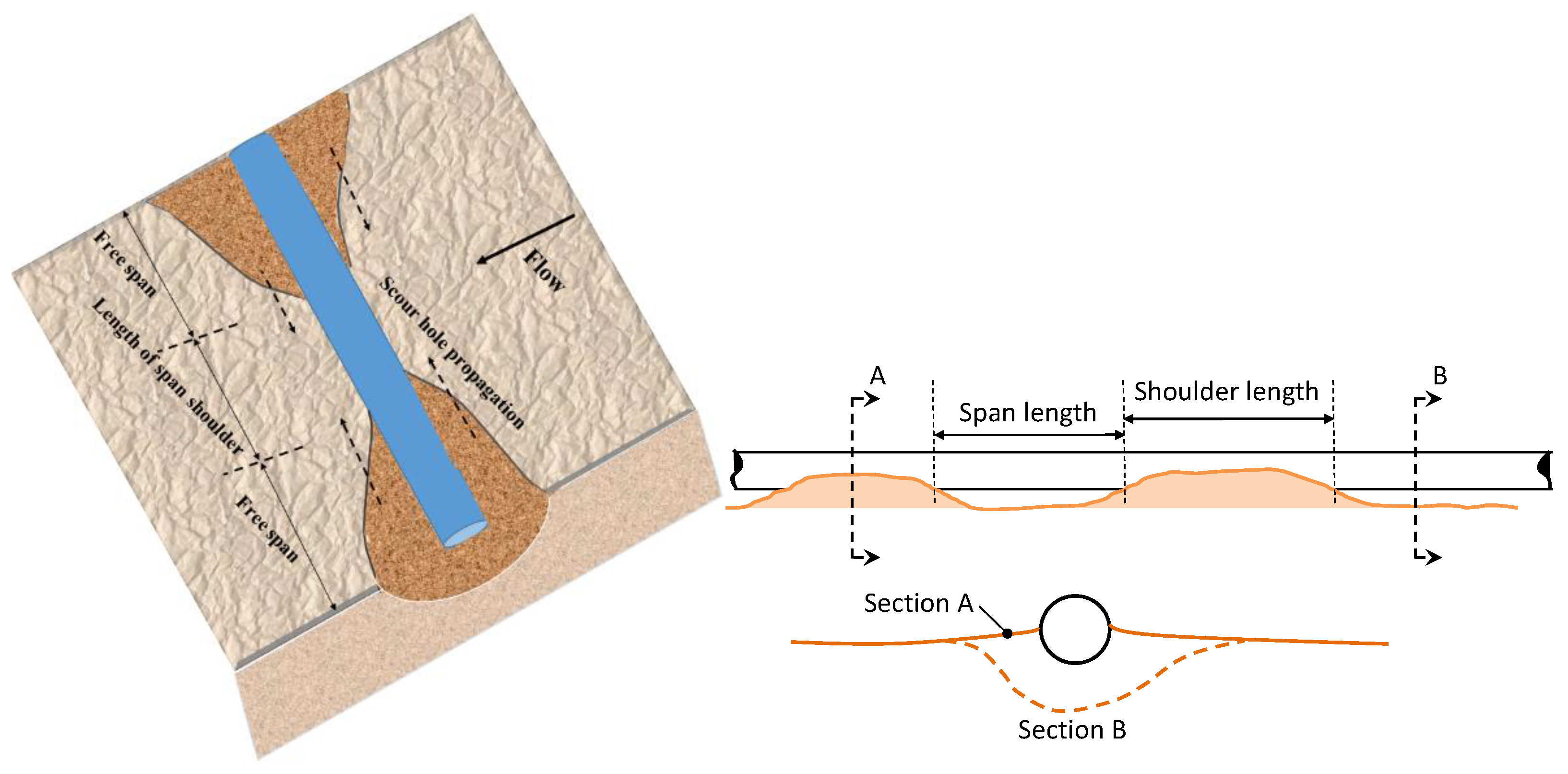
Figure 1. Schematic drawing of 3D scour hole propagation with free span expansion at a submarine pipeline (on the left); longitudinal and cross-section (i.e., Section A and Section B) views for a submarine pipeline prone to scour (on the right).
Applsci 11 03792 g001
Figure 2. Schematic diagram of onset scouring process for submarine pipelines under currents. (a) Vortex A in front of the pipe, Vortex B in the corner downstream of the pipe, and the largest Vortex C behind the pipe; (b) vortex shedding that forms after the scour develops.
Applsci 11 03792 g002
Figure 3. Schematic drawing of scouring vortices due to waves at a submarine pipeline. Wake vortexes downstream of the pipeline (a,b) due to oscillatory flow.
Applsci 11 03792 g003
Figure 4. Frequency and cumulative relative frequency for the independent non-dimensional variables.
Applsci 11 03792 g004
Figure 5. Performance of AI models in the prediction of V H * for: (a) Training and (b) testing stage.
Applsci 11 03792 g005
Figure 6. Performance of AI models in the prediction of V L * for: (a) training and (b) testing stage.
Applsci 11 03792 g006
Figure 7. Performance of AI models in the prediction of V R * for: (a) Training and (b) testing stage.
Applsci 11 03792 g007
Figure 8. Variations of V H * against e / D at: (a) KC = 8.7 and α = 0°, (b) KC = 15.8 and α = 0°, (c) KC = 18.0 and α = 0°, (d) KC = 15.8 and α = 30°, (e) KC = 18.0 and α = 30°, (f) KC = 18.0 and α = 15°, and (g) KC = 15.8 and α = 45°.
Applsci 11 03792 g008aApplsci 11 03792 g008b
Figure 9. Variations of V R * against e / D at KC from 8.7 to 18.0 and α = 0° for: (a) M5MT, (b) GEP, (c) EPR, and (d) MARS.
Applsci 11 03792 g009
Figure 10. Variations of V R * against KC at e / D from 0.1 to 0.4 and α = 0° for: (a) M5MT, (b) GEP, (c) EPR, and (d) MARS.
Applsci 11 03792 g010
Figure 11. Variations of V L * against e / D at KC from 8.7 to 18.0 and α = 0° for: (a) M5MT, (b) GEP, (c) EPR, and (d) MARS.
Applsci 11 03792 g011
Figure 12. Variations of V L * against KC at e / D from 0.1 to 0.4 and α = 0° for: (a) M5MT, (b) GEP, (c) EPR, and (d) MARS.
Applsci 11 03792 g012
Table 1. Basic statistical properties of the variables under study for AI modeling.
Dimensional VariablesMinimumMaximumAverageStandard Deviation
e [mm]5.020.011.975.445
U w [m/s]0.30.50.400.068
T [s]1.52.01.790.193
V H [mm/s]1.66.53.321.289
V R [mm/s]1.45.73.321.215
V L [mm/s]1.56.13.321.210
Dimensionless VariablesMinimumMaximumAverageStandard Deviation
s i n α [-]0.100.710.320.263
e / D [-]0.100.21430.08930.0893
K C [-]8.7018.0014.683.698
θ w [-]0.180.300.270.051
V H * [-]1.275.162.641.025
V R * [-]1.194.852.640.961
V L * [-]1.114.532.640.965
Table 2. Statistical performances of the AI models in the estimation of V H * .
AI ModelsTraining Stage
IOASSEMAESIADR
M5MT0.94680.06120.08860.09741.0090
GEP0.92440.01110.10560.11581.0039
EPR0.97990.00300.05500.05991.0026
MARS0.94680.00680.08260.10161.0068
AI ModelsTesting Stage
IOASSEMAESIADR
M5MT0.94300.13230.06440.06440.9682
GEP0.90840.21430.08930.08930.9621
EPR0.82370.41240.12540.19880.9260
MARS0.95060.11560.09120.10480.9476
Table 3. Statistical performances of the AI models in the estimation of V L * .
AI ModelsTraining Stage
IOASSEMAESIADR
M5MT0.98770.03870.06720.07721.0277
GEP0.96800.10010.10270.12741.0242
EPR0.98830.03690.07540.07711.0085
MARS0.99500.01570.03740.05040.9993
AI ModelsTesting Stage
IOASSEMAESIADR
M5MT0.98960.04490.06440.04811.0520
GEP0.99110.03840.05440.06110.9987
EPR0.96930.13220.09440.10521.0624
MARS0.98280.07380.08700.06801.0729
Table 4. Statistical performances of the AI models in the estimation of V R * .
AI ModelsTraining Stage
IOASSEMAESIADR
M5MT0.98010.07880.07280.10461.0163
GEP0.97600.09530.11990.11471.0294
EPR0.99130.03450.10300.06921.0113
MARS0.98310.06700.10300.09641.0050
AI ModelsTesting Stage
IOASSEMAESIADR
M5MT0.94350.15810.13560.16010.9955
GEP0.93290.18920.15250.17551.0020
EPR0.93560.18160.15000.17131.0503
MARS0.96700.08550.10860.16010.9578
Table 5. SSE values for the considered AI models when predicting V H * at various e / D ratios.
K C   and   α ValuesSSE Values for AI Models
M5MTGEPEPRMARS
K C = 8.7 and α = 0 ° 0.3000.4350.8430.161
K C = 15.8 and α = 0 ° 0.0180.0400.0810.078
K C = 18.0 and α = 0 ° 0.1470.2760.0180.142
K C = 18.0 and α = 15 ° 0.0490.0180.0400.010
K C = 15.8 and α = 30 ° 0.0110.0470.0030.063
K C = 18.0 and α = 30 ° 0.0310.0540.0280.040
K C = 15.8 and α = 45 ° 0.0050.0350.0060.054
Table 6. SSE values for the considered AI models when predicting V R * at various e / D ratios and K C values.
AI Models SSE   Values   for   e / D Varying
K C = 8.7 K C = 15.8 K C = 18.0
M5MT0.03880.20380.0271
GEP0.06220.26020.0827
MARS0.04830.08440.1490
EPR0.01680.01320.0969
AI Models SSE   Values   for   K C Varying
e / D = 0.1 e / D = 0.2 e / D = 0.3 e / D = 0.4
M5MT0.04800.09480.02440.1924
GEP0.03490.12980.04160.3338
MARS0.06290.16620.05440.0920
EPR0.03550.01060.00350.1197
Table 7. SSE values for the considered AI models when predicting V L * at various e/D ratios and KC values.
AI Models SSE   Values   for   e / D Varying
K C = 8.7 K C = 15.8 K C = 18.0
M5MT0.08740.09580.0488
GEP0.05020.10370.1627
MARS0.06180.18470.0563
EPR0.06060.04940.0272
AI Models SSE   Values   for   K C Varying
e / D = 0.1 e / D = 0.2 e / D = 0.3 e / D = 0.4
M5MT0.07250.09590.06580.0751
GEP0.18040.08030.01880.1425
MARS0.21890.12600.05260.0063
EPR0.07200.06170.02070.0286
Publisher’s Note: MDPI stays neutral with regard to jurisdictional claims in published maps and institutional affiliations.