EM-Driven Multi-Objective Optimization of a Generic Monopole Antenna by Means of a Nested Trust-Region Algorithm

Featured Application

Determination of trade-offs between conflicting design objectives in order to verify usefulness of the antenna for a range of application scenarios.

Abstract

Antenna structures for modern applications are characterized by complex and unintuitive topologies that are difficult to develop when conventional, experience-driven techniques are of use. In this work, a method for the automatic generation of antenna geometries in a multi-objective setup has been proposed. The approach involves optimization of a generic spline-based radiator with an adjustable number of parameters using a nested, trust region-based algorithm. The latter iteratively increases the dimensionality of the radiator in order to gradually improve its performance. The method has been used to generate a set of nine antenna designs, representing a trade-off between minimization of reflection within 3.1 GHz to 10.6 GHz and a reduction of size. The properties of the optimized designs vary along the Pareto set from −10 dB to −20 dB and from 230 mm² to 757 mm² for the first and second objectives, respectively. The presented design approach has been validated against a genuine, population-based optimization routine. Furthermore, the smallest Pareto-optimal design has been compared to the antennas from the literature.

1. Introduction

Ultra-wideband (UWB) antennas belong to the key components of modern location and tracking systems capable of providing centimeter-level accuracy [1,2,3,4,5,6]. For the mentioned services, the radiators may find application not only to data exchange, but also as energy harvesting devices that provide the necessary power for sensors [7,8,9,10]. A variety of application scenarios for tracking and location devices impose a range of potential requirements on antenna performance (in terms of field and electrical properties), as well as its dimensions (small footprint or specific shape) [10,11,12,13,14,15]. Consequently, a coherent system often comprises a range of antenna solutions.

The development of radiators for UWB applications is widely covered in the available literature [16,17,18,19,20,21,22,23,24]. Conventional design solutions include a range of planar components, such as monopoles [17,18] or dipoles [19,20] as well as volumetric structures [21,22]. Other antennas implement non-standard features that permit performance enhancement by excluding or including specific frequency bands [18,23] or implementing composite topologies to achieve multiple-input multiple-output capability [24,25]. Although the discussed antennas are characterized by varying dimensions or performance, their geometries stem from the mentioned basic topologies [16,17,18,19,20,21,22,23,24]. Consequently, enhanced functionality of the latter is often achieved through the introduction of specific geometry abbreviations (e.g., slots [23], stubs [24], perforations [11], or combinations thereof [16]). The modifications are predominantly introduced as a result of manual or semi-manual development, realized in a trial-and-error manner and oriented toward balancing the complexity and performance or size of the radiator [23,24].

Other approaches to the generation of an antenna structure involve representation of its geometry using a set of characteristic points interconnected by lines or appropriately defined curves [26,27,28,29,30]. Alternatively, the topology can be defined using a binary matrix (often with overlapping components with variable dimensions) [31,32,33], [34] where zeros and ones correspond to the areas with etched or continuous metallization [32]. Contrary to conventional radiators, antenna topologies described using generic models are predominantly determined using optimization methods [35,36,37,38,39]. Notwithstanding, the applicability of numerical algorithms to the generation of unconventional geometries is often demonstrated based on relatively simple, single-objective problems [28,29]. Furthermore, the optimization of generic models is normally undertaken using population-based routines (e.g., particle swarm optimization, genetic algorithms, or ant colony methods), which require thousands of evaluations to obtain the final solution [31,35,38,40]. To put that into perspective, in [41], the particle swarm algorithm required a total of 248 EM simulations to solve a set of 12 problems represented using only one input parameter. In [42], the same method required over 1400 model evaluations to find an optimal design of frequency selective surface represented using three adjustable variables. Due to the high evaluation cost (being in the order of minutes to hours), the application of conventional, population-based routines for the EM-driven optimization of antennas defined using generic models is impractical from a computational standpoint.

The design of modern antennas is a multi-objective (MO) problem, where a set of performance or geometry requirements is to be simultaneously fulfilled [38,43,44]. Conventional approaches to MO tasks involve conversion of the performance requirements into a single-objective function using aggregation techniques, penalty components, or design constraints [35,39,43]. The design task, formulated in this manner, can be solved using conventional single-objective routines [35,43]. On the other hand, aggregation techniques provide only one solution to the problem per algorithm run, whereas the quality of the result depends on the weights assigned to individual figures of interest [35]. Alternatively, MO optimization can be performed using the genuine MO algorithms [39,43]. The latter ones are especially useful when the designer’s priorities are not clearly defined, as they provide a set of solutions representing trade-offs between the requirements. Such cognitive studies are useful from the perspective of gaining a detailed insight into the capabilities of the antenna, with respect to the desired application scenarios or environments [45]. Although multi-objective problems could be solved using population-based metaheuristic methods, their practical applications are limited to rather simple structures due to the prohibitive computational cost [35,37]. Less numerically demanding routines involve the execution of evolutionary algorithms on the approximation models. Due to the curse of dimensionality [46], the usefulness of approximation models and metaheuristics for reliable MO optimization is limited either to low-dimensional structures or narrow search spaces [43,47]. Notwithstanding, the mentioned methods proved to be useful for solving problems characterized by over a dozen design parameters [43]. Alternatively, MO design can be handled using dedicated heuristic approaches oriented toward the sequential generation of Pareto-optimal solutions [43,47]. Nonetheless, neither of the mentioned methods are suitable for handling antenna models characterized by a flexible number of adjustable parameters.

The above considerations indicate that contemporary UWB antennas can be categorized into a few classes [16, 17,18,19,20,21,22,23,24]. The topologies from each group are similar except for features such as slots or stubs that are normally introduced as a result of manual, greedy search-based studies to alter the functionality of the structure. In this regard, representation of the antenna using a generic model might be useful for the automated development of its topology regarding the imposed performance and geometry requirements. Although “universal” antenna models have been reported in the literature, they lack flexibility in terms of the number of degrees of freedom used for their representation. Consequently, they are either too simple or too complex (parameter-wise) to obtain compromise designs. The application of generic topology (or its derivatives) for a range of application scenarios should reduce the cost of system development, as well as its time to market. Unfortunately, the available MO routines are inadequate for handling models with flexible parameterization due to the lack of mechanisms for the adjustment of problem dimensionality in the course of the optimization process. The motivation of this work is to address the mentioned challenges.

In this paper, a generic EM model of a planar antenna with flexible parameterization is presented. The structure is optimized in a bi-objective setup concerning minimization of in-band reflection within a 3.1 GHz to 10.6 GHz band and size. A set of designs, representing the trade-off between the requirements, is obtained using a novel framework that sequentially generates candidate solutions. The latter are refined in a nested trust region-based optimization loop that enables one to gradually increase the number of parameters. The proposed model and optimization framework are demonstrated through the generation of nine Pareto-optimal designs. Their geometries are represented using 30 to 46 input parameters. The variability of the antenna’s in-band performance and size along the Pareto set is from −10.3 dB to −20.5 dB (over 10 dB) and from 230 mm² to 757 mm² (almost 70 percent), respectively. The presented algorithm has been compared against other population-based metaheuristic routines in terms of optimization cost and the quality of obtained solutions. Numerical validation of the generated designs and comparisons of the smallest obtained UWB structure with the state-of-the-art compact antennas are also provided.

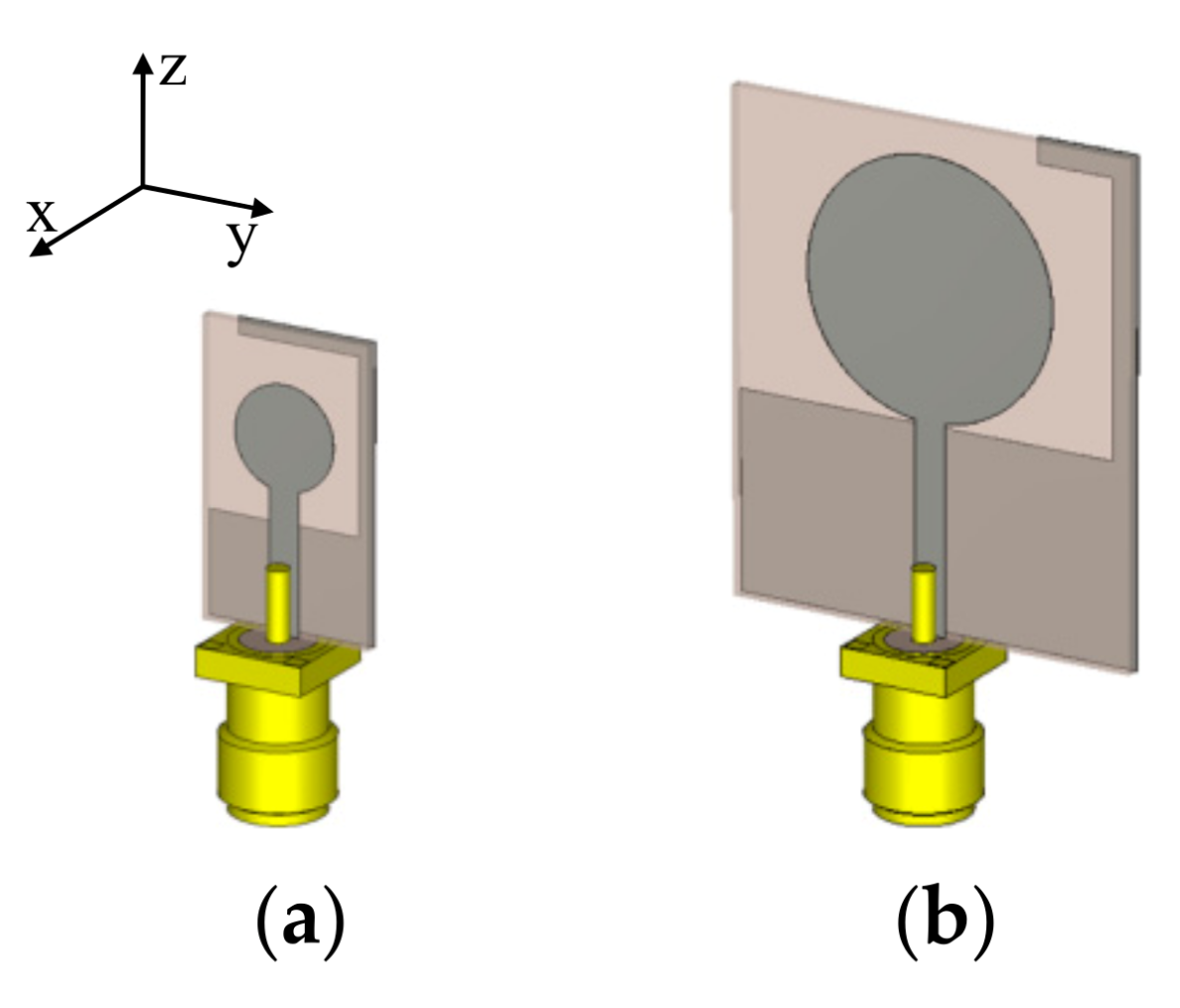
2. Generic UWB Monopole Antenna

Consider a planar monopole antenna, shown in Figure 1. The structure consists of a driven element in the form of a spline-parameterized radiator fed through a microstrip line. The ground plane edge oriented toward the radiating component is also implemented in the form of a spline curve. The presented topology generates closely located resonant modes, which contribute to the broadband behavior [48,49]. Furthermore, the bandwidth-related performance is enhanced using an L-shaped ground plane stub, which improves the impedance matching of miniaturization-oriented designs [24]. The structure is implemented on a Rogers RO4003 dielectric substrate with a permittivity of 3.58, thickness of 0.813 mm, and loss tangent of 0.0027. The vector of the antenna input parameters is y = [y_a y_g y_r]^T, where y_a = [X l_f l₁ l_2r w₁ o_r]^T, y_g = [y_g.1 … y_g.L]^T and y_r = [y_r.1 … y_r.L]^T (L = 50 represents the number of points used to represent the ground plane and radiator in the antenna model). The relative variables are l₂ = (X − w₁)l_2r, Y = l₁ + w₁, l_fr = min{0.5X, 0.5(Y − l_f)}, o = 0.5X + o_r. Dimension w_f = 1.8 remains fixed to ensure 50 Ohm input impedance. The unit for all variables except dimensionless l_2r is mm. It should be noted that vectors y_g = Y·z_g, and y_r = S·z_r, where S = min{0.5(X − o_r), 0.5(Y − l_f)} represent the characteristic points (so-called knots) of the spline curves used to define the ground plane and radiator, respectively (see Figure 1). To ensure the structure consistency, the gap between each knot y_g and y_r is even. Hence, the vectors denote the relative distance of the curve from the reference point (edge of the substrate for y_g and center of the radiator for y_r, respectively; Figure 1). It is worth emphasizing that y_r represents axial dimensions, as the parameters of the radiator are defined in a cylindrical coordinate system. The EM model of the antenna structure R is implemented in CST Microwave Studio and evaluated using its time domain solver.

The presented antenna supports flexible parameterization. In other words, the number of adjustable variables used for representation of the structure geometry can be changed in the course of the design process. The rationale behind this feature is that—when the generation of compromise design solutions is considered—the initial search space ranges are set to be large to ensure that the optimal designs are captured within them. The application of conventional (population-based) methods for exploration of the search space with wide parameter ranges is numerically impractical due to the tremendous number of iterations required for convergence [38,43]. Having a model with adjustable dimensionality, one can narrow down the search space to the region of interest using a relatively small number of parameters. The promising region can be further exploited through optimizations of the model characterized by gradually increasing dimensionality. Flexible parameterization has been implemented through implicit handling of the input variables. Let x_d = [y_a x_g.d x_r.d]^T, where x_g.d = [x_g.1 … x_g.d]^T, x_r.d = [x_r.1 … x_r.d]^T, d = 1, …, L represent the d-knot spline curve used to represent the antenna ground plane and radiator, respectively. Note that when d < 4, x_g.d = x_g.1 and x_r.d = x_r.1, because the implementation of the spline used in this work requires at least four knots. The change of the antenna dimensionality is realized through the interpolation of x_g.d and x_r.d to z_g = z_g.L and z_r = z_r.L vectors, respectively. The process can be defined as follows:

$$z_{\left\{g,r\right\}}\leftarrow sp\left(x_{\{g,r\}}{}_{.d},L\right)$$

(1)

where sp is the function that realizes L-point spline-based interpolation of the d-dimensional input vector. The conversion process is transparent to the design optimization algorithm. The lower and upper bounds for the structure optimization are l_b = [6 4 10 0.05 0.5 −1 l_g.d l_r.d]^T and u_b = [30 15 30 1 2.5 1 u_g.d u_r.d]^T, where l_g.d = [0.2 … 0.2]^T, l_r.d = [0.1 … 0.1]^T, and u_g.d = [0.8 … 0.8]^T, l_r.d = [1 … 1]^T.

3. Design Methodology

In this section, the proposed design methodology is explained. To make the paper self-contained, a short discussion of the multi-objective design problem, followed by a brief description of the utilized optimization algorithm, are provided here. Next, the introduced multi-objective optimization method that permits a gradual increase of the number of antenna parameters is described. The section is concluded with the summary of the presented design framework. Numerical results are provided in Section 4.

3.1. Multi-Objective Design Problem

The multi-objective design problem can be defined as follows [39]:

$$x^{*}\in \arg \underset{x\in X}{\min }F\left(x\right)$$

(2)

where x = x_d (see Section 2) denotes the vector of the design parameters, X is the feasible region of the search space, and x^* represents the optimal design. The objective functions are given as

F(x) = [F₁(x), …, F_q(x)]^T

(3)

where q = 1, …, Q. Note that F(x) = F(R(x)), where R(x) is a vector of responses obtained from EM evaluation of the antenna model at the design x. The responses may represent the electrical performance (e.g., reflection over a frequency range or isolation between radiators), field (e.g., single-direction gain over the frequency or radiation pattern at the given frequency), or geometry (e.g., footprint or volume) of the structure. If Q > 1, the conventional notion of performance improvement known from single-objective optimization (i.e., the one based on direct comparison of the objective function responses obtained for candidate solutions) is not applicable [39]. Instead, designs can be compared using a domination relation [39]. One can say that the design x₁ dominates over x₂ if F_q(x₁) ≤ F_q(x₂) for all q and F_q(x₁) < F_q(x₂) for at least one objective. A design x_q^* is optimal in the Pareto sense if there is no other design x_r^* (q ≠ r), such that x_r^* dominates over x_q^*. The solution to the multi-objective problem is a set of Pareto-optimal designs. For a more detailed description of the MO optimization concept, see [35,39,43].

3.2. Nested Optimization with a Variable Number of Design Parameters

Although conventional global-optimization algorithms proved to be useful for solving complex problems, they suffer from an unacceptable numerical cost, associated with the tremendous number of model evaluations required to find the optimal designs. On the other hand, deterministic algorithms (such as gradient or pattern search methods [36,50]) are often characterized by a lower computational cost yet limited capability in terms of escaping from local minima. In this work, the problem is mitigated by performing a series of optimizations in a nested loop. The latter gradually increases the number of design variables, first to identify and then to exploit the region of the search space of interest. The analogy to this approach, from the perspective of the design objective space, is observation of the landscape from a high altitude where the amount of visible details is limited. With each iteration of the nested loop (that is associated with an increasing the number of parameters), the “altitude” decreases, which allows the algorithm to “identify” more details of the landscape and improve the design response.

Let d = [d₁ … d_n … d_N]^T, d_n = 1, …, L, n = 1, …, N represent the set defining the number of spline parameters (positive integer values) used to represent the ground plane and radiator, respectively. In each step, the final d_n dimensional design x_dn^*, obtained in the nth nested iteration, is used as a starting point for the n + 1 step. Assuming that the vector d is defined, n is set, and the initial design x_dn^* is available, the nested optimization can be summarized as follows:

1.

Set x_dn+1⁽⁰⁾ ← sp(x_dn^*,d_n+1) (see Section 2);

2.

Find design x_dn+1^* using x_dn+1⁽⁰⁾ as a starting point for optimization;

3.

If n = N, END; otherwise, set n = n + 1 and go to 1.

It should be noted that the size N of vector d substantially affects the algorithm cost, as the optimization process is reset at each iteration n = 1, …, N. On the other hand, the number of iterations and step size between d_n and d_n+1 can be adjusted so as to mitigate the risk of getting stuck in a poor local optimum while managing the optimization cost at the acceptable level. Conceptual visualization of the objective function (a so-called feature) and design spaces for the structure, represented using the increasing number of parameters, is shown in Figure 2.

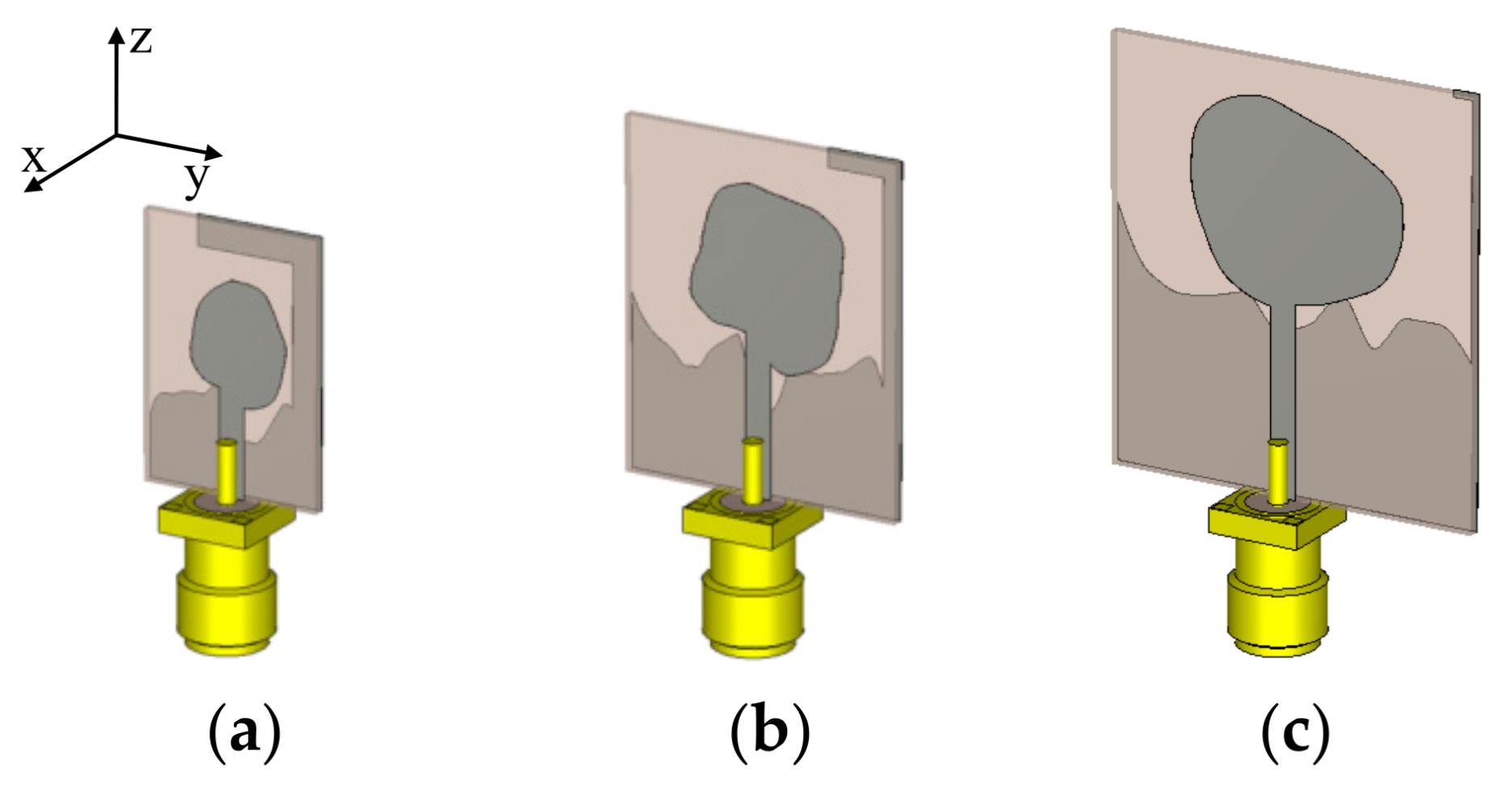
3.3. Generation of Trade-Off Designs

The presented bi-objective optimization algorithm involves two stages: (i) generation of the extreme (or corner) designs and (ii) sequential determination of the Pareto set using constrained optimizations. The first corner solution is obtained by solving the following minimization problem:

$$x_1{{}_{.d_n}}^{*}=\arg \underset{x_{d_n}\in X}{\min }{F}_1\left(x_{d_n}\right)$$

(4)

Note that Equation (4) involves optimization of the structure in regard to a single objective. The second design is obtained through constrained optimization, oriented toward minimization of the second performance criterion:

$$x_{2.d_n}{}^{*}=\arg \underset{\begin{array}{c}{x}_{d_n}\in X\\ F_1\left(x_{d_n}\right)\le F_{1.\max }\end{array}}{\min }{F}_2\left(x_{d_n}\right)$$

(5)

The goal of Equation (5) is to minimize F₂ while ensuring that the response of the optimized design x_2.dn^* does not violate the defined threshold F_1.max. The reasoning behind the introduction of a design constraint is to permit minimization of the second objective while maintaining the response regarding F₁(x_dn) at an acceptable level. Generation of the extreme points is conceptually illustrated in Figure 3.

In the second stage, the algorithm sequentially identifies the Pareto designs. In each step, the new points are obtained between the already existing optimal solutions. Let x_p.dn^* (p = 1, …, l_k; l_k = 2^k−1 + 1) represent the Pareto designs obtained in the k − 1 iteration, where k = 1, …, K. It should be noted that l₀ = 2 refers to two corner designs—x_1.dn^*, x_2.dn^*—found in the first design stage. The candidate solutions are determined as follows:

$$x_{c.d_m}^{\left(0\right)}=\left. [x^{*}{{}_p}_{.d_m}+x^{*}{}_{p+1.d_m}\right]/2$$

(6)

where c = l_k + b and b = 1, …, l_k − 1. It should be noted that the reference designs in Equation (6) are approximated using d_m variables. Hence, the cth candidate design can be generated even when using x^*_p.dn and x^*_p+1.do, d_n ≠ d_o (o = 1, …, N). This is ensured by interpolating the reference designs’ dimensionality as x_p.dm⁽⁰⁾ ← sp(x_p.dn^*, d_m), x_p+1.dm⁽⁰⁾ ← sp(x_p+1.do^*, d_m) (see Section 2). The obtained candidate solutions are utilized as starting points for constrained optimization:

$$x_{c.d_n}{}^{*}=\arg \underset{\begin{array}{c}{x}_{c.d_n}\in X\\ F_2\left(x_{c.d_n}\right)\le F_{2.c.\max }\end{array}}{\min }{F}_1\left(x_{c.d_n}\right)$$

(7)

The goal of Equation (7) is to minimize the objective function F₁ while maintaining the structure response with respect to the second objective below the specified threshold. The latter is set to F_2.c.max = 0.5(F₂(x_p.dn^*) + F₂(x_p+1.dn^*)). In order to facilitate generation of the Pareto set, the constraint on F₂ is implemented in the form of a penalty coefficient included with the objective function. The process in Equation (7) is performed in a nested optimization loop as shown in Section 3.2. As already mentioned, such an approach allows one to gradually increase the quality of the Pareto designs by appropriate adjustment of the antenna dimensionality. Finally, the designs {x_p.dn^*}_{p = 1, …, lk} and {x_c.dn^*}_{c = lk + (1, …, lk−1)} are concatenated as {x_1.d^*, x_b+1.dn^*, x_2.dn^*, x_b+2.dn^*, …, x_lk−1.dn^*, x_2lk−1.dn^*, x_lk.dn^*} and reindexed to {x_1.d^*, x_2.dn^*, x_3.dn^*, x_4.dn^*, …, x_2lk−3.dn^*, x_2lk−2.dn^*, x_2lk−1.dn^*}. The discussed optimization routine (see Figure 4 for a block diagram) can be summarized as follows:

1.

Set the initial designs x_1.d1⁽⁰⁾ and x_2.d1⁽⁰⁾; set d = [d₁ d₂ … d_m … d_n … d_N]^T;

2.

Obtain x_1.dn^* and x_2.do^* (n ≤ N, o ≤ N) by solving Equations (4) and (5) in a nested loop (see Section 3.2);

3.

Set k = 1;

4.

Set p = 1;

5.

Set x_p.dm^* ← sp(x_p.dn^*, d_m), x_p+1.dm^* ← sp(x_p+1.do^*, d_m) (see Section 2), and then calculate x_c.dm⁽⁰⁾ and set F_2.c.max;

6.

Generate x_c.dn^* by solving Equation (7) in a nested optimization loop;

7.

If p = l_k, go to 7; otherwise set p = p + 1 and go to 5;

8.

Concatenate the designs as {x_1.d^*, x_b+1.dn^*, x_2.dn^*, x_b+2.dn^*, …, x_lk−1.dn^*, x_2lk−1.dn^*, x_lk.dn^*}, and then reindex the resulting set;

9.

If k = K, END; otherwise, set k = k + 1 and go to 4.

In the first stage of the presented framework, the initial designs x_1.d1⁽⁰⁾ and x_2.d1⁽⁰⁾ are obtained using a greedy search-based topology adjustment. The goal of the procedure is to find reasonable starting points for the optimization process. Upon identification of the initial designs, the generation of the Pareto set is handled by the above-outlined routine.

It is worth mentioning that the concept of generating intermediate designs is similar to the one presented in [47]. Here, however, the bisections are used only for the generation of candidate designs, which are further refined by means of constrained optimization. Furthermore, the algorithm of [47] does not support increasing the dimensionality of the problem in the course of structure optimization. Owing to the identification of new designs between the already existing ones, the algorithm allows for obtaining a Pareto set characterized by relatively even separation between the consecutive solutions (in the objective function space). Generation of the Pareto designs using the discussed algorithm is conceptually illustrated in Figure 5.

3.4. Optimization Engine

The optimization engine used in this work for solving Equations (4), (5), and (7) is a local gradient method [36]. The algorithm is embedded in a trust region (TR) framework [37]. The latter generates a series (i = 1, 2, 3, …) of local models around what is currently the best design x⁽ⁱ⁾ in order to gradually approximate the optimal solution to be found. The TR-based optimization is defined as [37]

$$x^{\left(i+1\right)}=\arg \underset{x:‖x-x^{\left(i\right)}‖\le r^{\left(i\right)}}{\min }F\left(G^{\left(i\right)}\left(x\right)\right)$$

(8)

where G⁽ⁱ⁾ is a first-order Taylor expansion model, given by [51]

$$G^{(i)}\left(x\right)=R\left(x^{(i)}\right)+J\left(x^{(i)}\right)\cdot \left(x-x^{(i)}\right)$$

(9)

where J(x⁽ⁱ⁾) represents the Jacobian generated around x⁽ⁱ⁾ using a large-step finite differentiation [51]. The TR radius r⁽ⁱ⁾ (i.e., the region around x⁽ⁱ⁾ for which the model is considered valid) is adjusted based on the calculated gain ratio [51]:

$$\rho =\frac{R\left(x^{(i+1)}\right)-R\left(x^{(i)}\right)}{G^{(i)}\left(x^{(i+1)}\right)-G^{(i)}\left(x^{(i+1)}\right)}$$

(10)

The candidate design x⁽ⁱ⁺¹⁾ is accepted only if ρ > 0. Otherwise, the iteration is reset. The radius is updated according to the standard rules [37]. The initial value r⁽⁰⁾ is controlled by the nested optimization loop (i.e., for n = 1, the radius is set to r⁽⁰⁾ = 1, whereas for n > 1, r⁽⁰⁾ = 1/d_n) (see Section 3.2). The algorithm is terminated either when the Euclidean distance between two consecutive designs or the radius are smaller than a specified threshold (i.e., ||x⁽ⁱ⁺¹⁾ − x⁽ⁱ⁾|| ≤ ε, or r⁽ⁱ⁺¹⁾ ≤ ε (here, ε = 10⁻²)). The algorithm can be summarized as follows:

1.

Set i = 0 and x⁽⁰⁾, then set r⁽⁰⁾ according to the iteration of the nested loop in Section 3.2;

2.

Generate the Jacobian J(x⁽ⁱ⁾) and construct the local approximation model G⁽ⁱ⁾;

3.

Find x⁽ⁱ⁺¹⁾ by solving Equation (8);

4.

Evaluate R(x⁽ⁱ⁺¹⁾) and calculate ρ;

5.

If ρ > 0.75, set r⁽ⁱ⁺¹⁾ = 2r⁽ⁱ⁾. If ρ < 0.25, set r⁽ⁱ⁺¹⁾ = r⁽ⁱ⁾/3;

6.

If ρ < 0, go to 3; otherwise, go to 7;

7.

If the termination condition is met, END; otherwise, set i = i + 1 and go to 2.

Owing to utilization of the Taylor model, the computational cost of the algorithm is low, as it requires d_n + 1 simulations of the R model per successful iteration. Additional evaluations are required for the steps that do not improve the objective function value. The justification for decreasing the initial radius when n > 1 is that with each iteration of the nested loop, the goal of the algorithm is to exploit the region identified in the previous step. For more comprehensive discussion on TR optimization methods, see [37,51].

4. Numerical Results

In this section, the presented antenna structure and design optimization algorithm are numerically validated. The design problem involves bi-objective optimization of the radiator for size reduction and minimization of reflection within the frequency band of interest. The obtained EM simulation results were verified based on evaluations performed using a frequency domain solver. Furthermore, the presented routine has been compared against a conventional multi-objective optimization algorithm in terms of computational cost and quality of the obtained Pareto designs. Finally, the smallest obtained antenna solution has been benchmarked against other structures from the literature. All computations have been performed using an Intel Xeon E5-2650 processor with 32 GB of RAM.

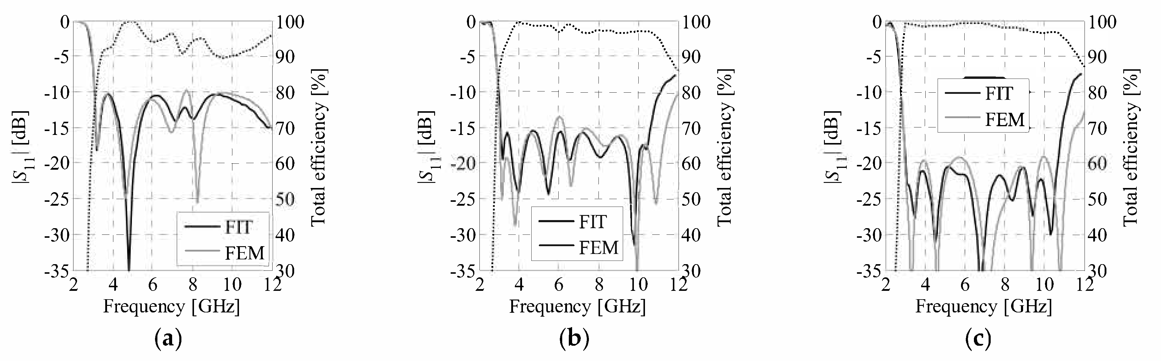
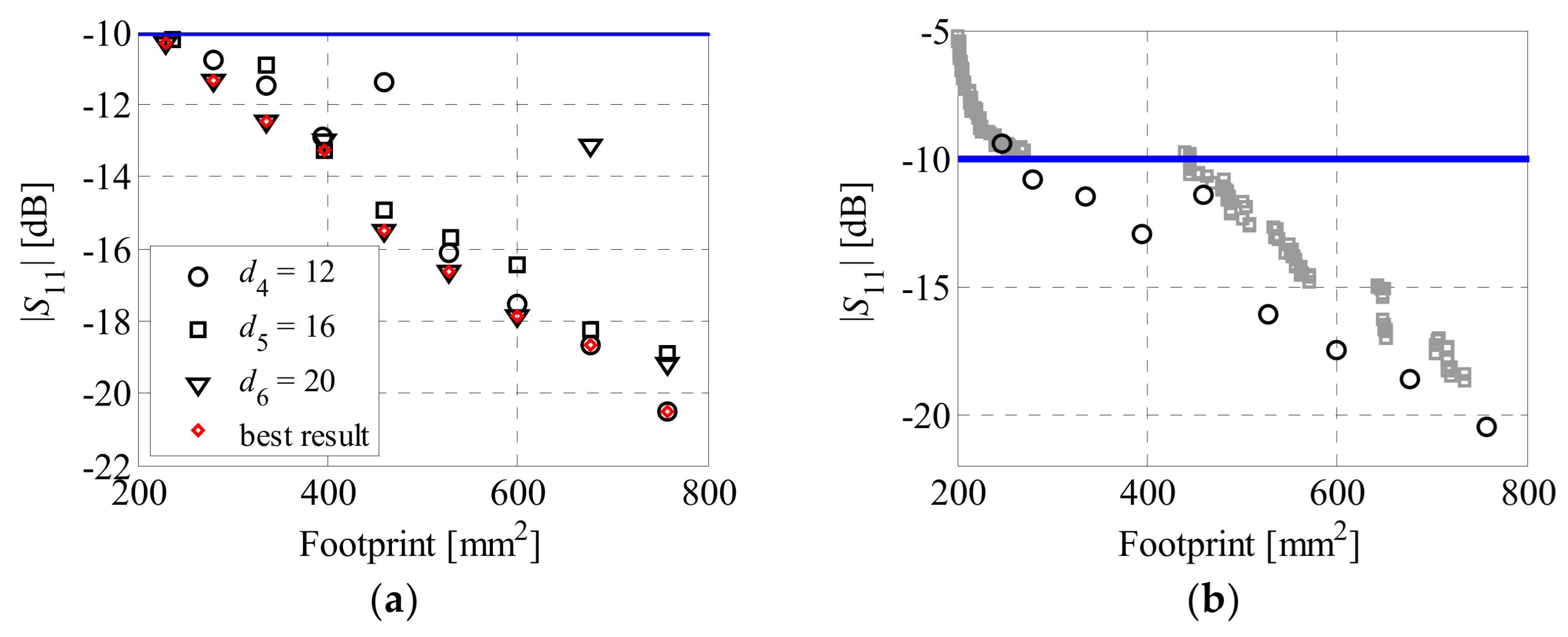
4.1. Bi-Objective Antenna Optimization

The design objectives for the considered antenna optimization problem included the following: the minimization of reflection F₁, such that|S₁₁| = |R(x)| = |R(x, f)|, where f = f_L, …, f_H denotes the frequency points at which the radiator is evaluated (f_L = 3.1 GHz, f_H = 10.6 GHz), as well as the reduction of the structure footprint F₂, defined as A(x) = X × Y rectangle (see Section 2).

The starting points for determination of the extreme Pareto designs were x_1.1⁽⁰⁾ = [10 6 16 0.8 1 0 0.35 0.6]^T and x_2.1⁽⁰⁾ = [24 10 27 0.2 1.5 0 0.4 0.8]^T. It is worth noting that, due to being represented using only one variable, the radiators and ground planes of the initial designs were in the forms of circles and rectangles, respectively. Both antenna geometries are shown in Figure 6. The objective function for optimization with respect to the first performance requirement was defined as

$$F_1\left(x\right)={\alpha }_1{E}_1\left(x\right)+\min \left\{0,E_2\left(x\right)\right\}$$

(11)

where

$$E_1\left(x\right)=\frac{1}{M}{{\displaystyle \sum \left|\frac{|S_{11}{|}_{f_v}-S_{\max }}{S_{\max }}\right|}}^2$$

(12)

$$E_2\left(x\right)=\max \left(\left|S_{11}\right|\right)+S_{\max }$$

(13)

Here, |S₁₁|_fv represents the reflection at M frequency points f_v ∈ f, the value of which was higher than the S_max = −15 dB threshold. Note that the definition of Equation (12) in the least squares sense provided smooth changes of the objective function values in the course of the optimization process [51]. On the other hand, E₁(x) = 0 when the antenna response was below S_max for all f_v points. In this case, the control over optimization was taken over by the min-max component in Equation (13). The scaling coefficient was set to α₁ = 10⁴ in order to ensure a smooth transition between the E₁(x) and E₂(x) functions. The second design objective was given as

$$F_2(x)={\alpha }_{2}A{(x)}^2+E_1\left(x\right)$$

(14)

where α₂ = 0.01 in order to ensure that the contribution of E₁(x) to F₂(x) was noticeable for a relatively small violation of S_max = F_1.max = −11 dB. It should be noted that for the majority of the antenna structures, a typical design requirement is to ensure that the reflection is below the −10 dB threshold. However, in practice, minimization of Equation (14) often leads to violation of the condition [43]. Setting a lower-than-required threshold S_max allowed us to ensure that |S₁₁| ≤ −10 dB within the frequency band of interest.

The vector representing the dimensionality of the antenna (spline-based features of the structure) was d = [d₁ … d₆]^T = [1 4 8 12 16 20]^T. Hence, the number of nested optimizations per corner solution was N = 6. Moreover, d_m = d₄ = 12 (see Section 3.3). Figure 7 shows the antenna responses (corner points) obtained at each stage of the nested loop. The optimized corner designs were x₁._d4^* = x_1.12^* = [26.07 10.56 28.56 0.06 0.5 0.51 0.38 0.44 0.46 0.41 0.47 0.39 0.36 0.44 0.43 0.42 0.43 0.59 0.78 0.77 0.71 0.73 0.81 0.75 0.65 0.72 0.9 0.88 0.78 0.75]^T and x_2.d6^* = x_2.20^* = [12.54 4.16 16.22 0.66 2.14 −0.19 0.35 0.37 0.33 0.27 0.22 0.2 0.2 0.2 0.2 0.23 0.4 0.37 0.34 0.35 0.34 0.34 0.32 0.32 0.31 0.23 0.46 0.5 0.53 0.52 0.48 0.44 0.45 0.5 0.55 0.61 0.7 0.73 0.66 0.62 0.65 0.64 0.69 0.74 0.73 0.64]^T, respectively. Note that the dimensionality of the extreme points was different (12 relative variables per feature—30 total—for x₁^* vs. 20–46 total for x₂^*), which was due to the lack of performance improvement from increasing the number of x₁ variables above 12. The obtained solutions were used as starting points for generation of the Pareto set. In the second design stage, the Pareto designs were obtained using an objective of the following form:

$$F_{1.c}\left(x\right)=F_1\left(x\right)+{\left(\max \left\{0,A(x)-A_c\right\}\right)}^2$$

(15)

The additive component of Equation (15) is a penalty coefficient activated when the threshold A_c = 0.5(A(x_m.d^*) + A(x_m+1.d^*)) is violated. In F₁(x), the parameter S_max = F_1.c.max (see Section 3.3). The number of algorithm iterations was set to K = 3. The candidate solutions for optimization were generated using Equation (6). The Pareto set, composed of two corner and seven intermediate designs {x_1.20^* x_2.20^* x_3.20^* x_4.20^* x_5.20^* x_6.20^* x_7.20^* x_8.12^* x_9.12^*}, and the frequency responses of the selected optimal solutions are shown in Figure 8. The obtained results indicate that the footprints of the optimized antennas ranged from 230 mm² (with an in-band reflection of −10.3 dB) to 757 mm² (reflection of −20.5 dB). Hence, the change in antenna size and frequency responses along the Pareto set were 527 mm² and 10.2 dB, respectively. It is worth noting that the miniaturization rate of the smallest antenna with reference to the largest one was almost 70%. The gain pattern responses were obtained for the selected antenna designs (i.e., x_1.20^*, x_9.12^* (corner designs), and x_5.20^* = [19.36 7.41 22.43 0.22 1.32 0.1 0.36 0.44 0.41 0.38 0.37 0.36 0.36 0.35 0.26 0.21 0.32 0.43 0.41 0.37 0.32 0.32 0.36 0.38 0.42 0.49 0.59 0.59 0.67 0.69 0.59 0.5 0.52 0.57 0.64 0.64 0.6 0.63 0.73 0.8 0.74 0.73 0.82 0.92 0.9 0.71]^T) (see Figure 9 for a visualization of the topologies). The characteristics shown in Figure 10 indicate that the x_1.20^* design was characterized by slightly more omnidirectional radiation patterns in the x–y plane and lower gain compared with the x_5.20^* and x_9.12^* geometries.

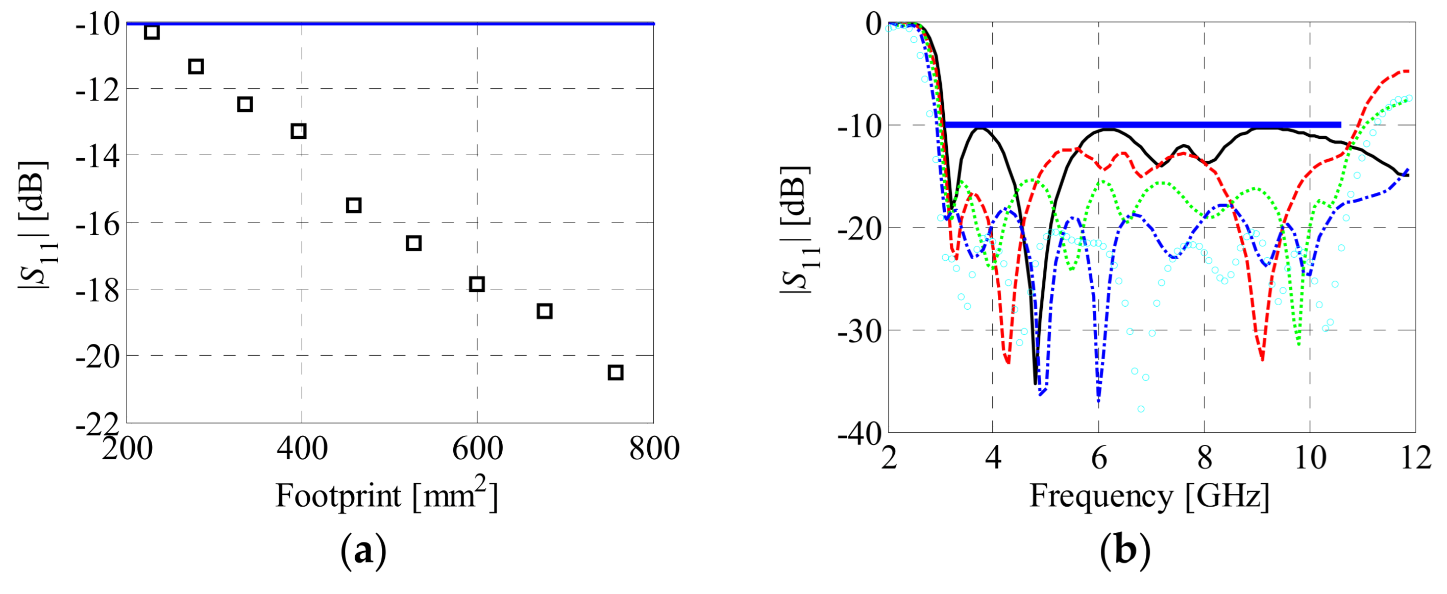
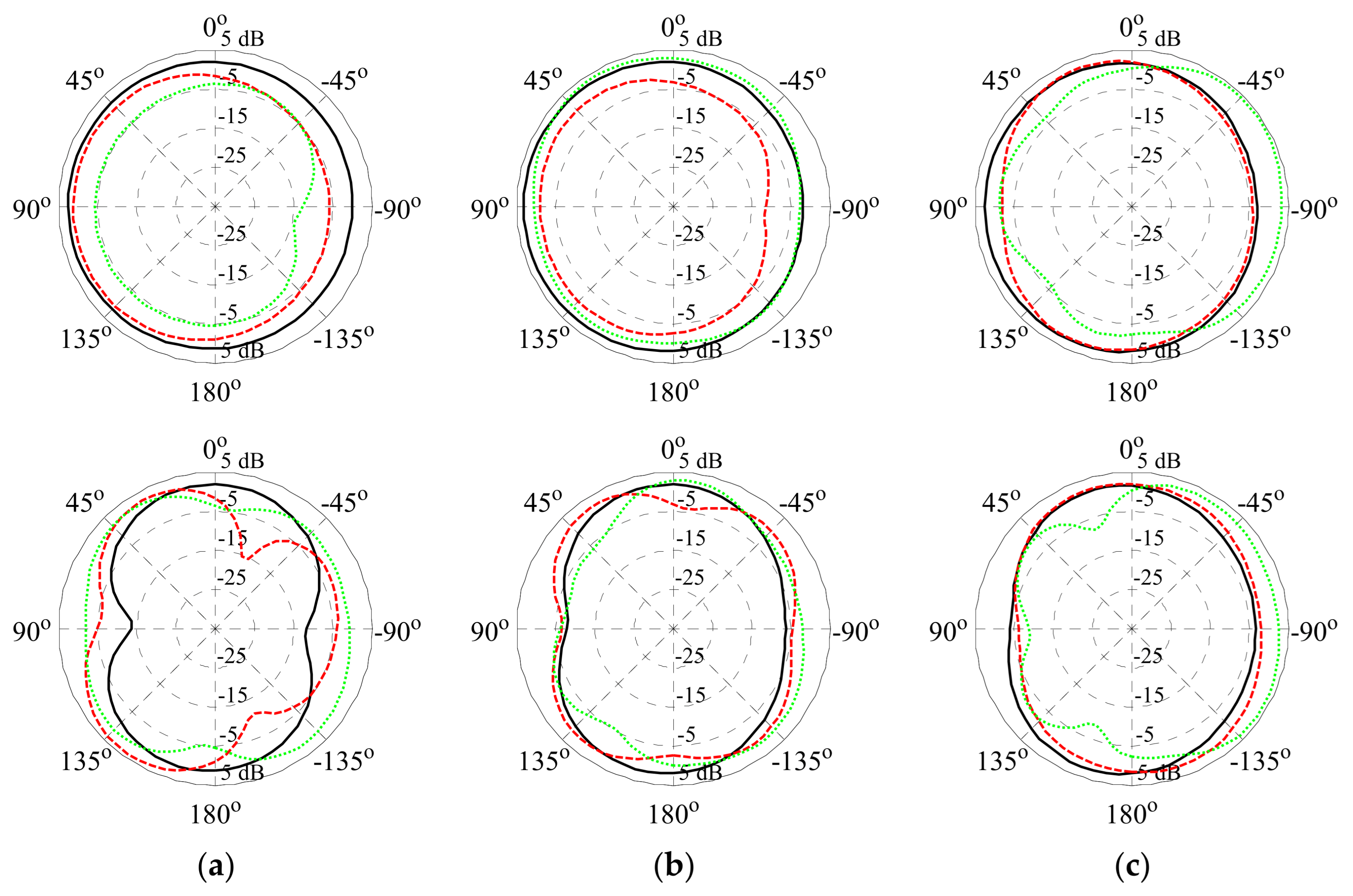
4.2. Comparisons and Discussion

To confirm the validity of the numerical results, the x_1.20^*, x_5.20^*, and x_9.12^* designs were evaluated using a frequency domain solver (finite elements method with adaptive meshing) implemented in CST Studio [52]. The response characteristics (shown in Figure 11) obtained using the time and frequency domain methods were similar, which indicates that the EM models used in the optimization process were valid. Furthermore, the plots of Figure 11 show that, at the lower corner frequency of 3.1 GHz, the x_1.20^*, x_5.20^*, and x_9.12^* designs featured radiation efficiencies of 76%, 89%, and 99%, respectively. Note that for the x_1.20^* design, an efficiency of over 90% was achieved above the 3.4 GHz frequency, which is considered acceptable, keeping in mind its small footprint. Overall, the considered antennas were characterized by average in-band efficiencies of 93%, 97%, and 98%, respectively. Clearly, the high values were due to the utilization of a low-loss substrate for implementation of the structures.

Figure 12a shows a comparison of the optimal solutions obtained at different iterations of the nested loop (represented using a varying number of parameters). As can be seen, for the majority of the designs, increasing the dimensionality resulted in improvement in the structure responses. However, for certain solutions, a larger number of variables led to performance degradation. This was due to insufficient precision of the spline approximation when the number of knots increased, which led to undesirable frequency shifts at the edges of the operational bandwidth. Notwithstanding this, for most of the designs, the imperfections were corrected by the optimization algorithm.

The computational cost of bi-objective optimization corresponded to 4389 evaluations of the EM antenna model (~159.7 h of CPU time). The cost breakdown, with emphasis on individual nested loops, is gathered in

Table 1. Cost breakdown of the multi-objective optimization of the spline-parameterized antenna.

Design	Number of Model Evaluations [R]						Total [R]	Total [h]
	n = 1	n = 2	n = 3	n = 4	n = 5	n = 6
x1.dn*	64	92	94	156	326	284	1016	36.97
x2.dn*	N/A	N/A	N/A	187	2	192	381	13.86
x3.dn*	N/A	N/A	N/A	158	41	145	344	12.52
x4.dn*	N/A	N/A	N/A	193	119	98	410	14.92
x5.dn*	N/A	N/A	N/A	128	198	146	472	17.18
x6.dn*	N/A	N/A	N/A	127	119	284	530	19.28
x7.dn*	N/A	N/A	N/A	158	41	238	437	15.90
x8.dn*	N/A	N/A	N/A	156	81	96	333	12.12
x9.dn*	56	46	118	156	40	50	466	16.96
Total	120	138	212	1419	967	1533	4389	159.71

. It should be noted that the average numerical expenses associated with the identification of a single Pareto-optimal design corresponded to about 488 R model evaluations, which is low when having in mind the dimensionality of the problem (up to 46 independent parameters). It is also worth noting that optimization of the designs represented using more than 30 variables amounted to 57% of the overall cost. For the sake of comparison, the antenna at hand was also optimized using a standard population-based multi-objective evolutionary algorithm (MOEA) with fitness sharing, mating restrictions, and Pareto dominance tournament selection [53]. The setup of the benchmark routine was as follows. The population size and the number of generations were set to 200 and 50 (a total of 10,000 EM simulations), respectively, whereas the probability of mutation and crossover were fixed at 0.2 and 0.5, respectively. Since the discussed algorithm did not support adjusting the antenna dimensionality, the number of parameters was set to 30 (i.e., d₄ = 12). Furthermore, the corner designs obtained using the method in Section 3 were included into the initial population. The latter was generated between the extreme points in order to narrow down the search space to the region of interest. Figure 12b shows a comparison of the designs obtained using both routines (the plots present the responses obtained for the antenna model, represented using 30 parameters). As can be seen, the algorithm of Section 3 outperformed the benchmark method in terms of performance of the resulting designs. More importantly, the number of R simulations required to obtain the final designs using the proposed algorithm amounted to 1889, which was 81% less compared to the cost of MOEA operation. Even when the optimization was performed in a nested loop, the cost of the presented algorithm (4389 EM simulations) was over two times lower compared with the benchmark routine (while providing noticeably better responses characterized by a more even spread between the extreme designs and better in-band reflection).

One should emphasize that the dimensions of the smallest Pareto-optimal antenna design were only 12.5 mm × 18.4 mm (footprint = 230.4 mm²). The structure was compared against other compact UWB monopoles from the literature in terms of size and bandwidth. For the sake of fair comparison, the dimensions of the considered structures were expressed in terms of the guided wavelength λ_g calculated for the lower corner frequency and the electrical performance of the substrates on which the considered radiators were implemented. The results gathered in

Table 2. Spline-parameterized antenna (x_1.20^*) in comparison with the benchmark designs.

Antenna	fL [GHz]	Bandwidth [GHz]	Dimensions [mm × mm]	Size [mm2]	Dimensions [λg × λg]	Footprint # [λg2]
[55]	2.9	6.6	32.0 × 36.0	1152	0.56 × 0.64	0.359
[56]	3.0	8.0	28.0 × 38.0	1064	0.51 × 0.69	0.352
[57]	3.1	8.4	14.5 × 28.0	406	0.27 × 0.52	0.140
[11]	2.9	19.3	25.0 × 17.0	425	0.44 × 0.30	0.132
[18]	3.0	7.8	10.0 × 32.5	325	0.18 × 0.59	0.106
[54]	3.0	7.6	10.0 × 25.0	250	0.17 × 0.43	0.073
[58]	3.1	8.3	7.00 × 25.0	175	0.13 × 0.47	0.061
This work	3.1	8.9	12.5 × 18.4	230	0.32 × 0.22	0.069

^# For fair comparison, the antenna size is expressed in terms of the guided wavelength corresponding to the substrate properties the design is implemented on.

indicate that the proposed structure was characterized by a competitive size while providing acceptable performance. Small dimensions make the design’s potential use not only for a range of mobile UWB sensors and IoT-based localization services, but also for body of area network applications [54].

5. Conclusions

In this work, a spline-based UWB monopole antenna with an adjustable number of parameters has been presented. The structure has been optimized in a bi-objective setup using an algorithm that enables sequential generation of the Pareto designs between the extreme solutions. Each step of the design process involves a trust region-based optimization of the structure in a nested loop. The latter gradually increases the dimensionality of the antenna. The trade-off solutions are generated through the optimization of candidate designs, determined from bisections between the already existing solutions. The proposed method was used to obtain a total of nine antenna designs, representing compromises between a minimization of reflection within 3.1 GHz to 10.6 GHz band and size reduction. The geometries of the optimized radiators were represented using 30 to 46 independent parameters. The performance and sizes of the final designs along the Pareto front varied from −10.3 dB to −20.5 dB and from 230 mm² to 757 mm², respectively. The method has been favorably validated against a genuine multi-objective optimization algorithm in terms of computational cost and the quality of the obtained solutions. Furthermore, the smallest Pareto-optimal antenna was compared against the state-of-the-art monopoles from the literature. The optimized radiator is characterized not only by competitive performance, but also a small footprint, which makes it of potential use for UWB sensors, mobile localization services, or body area networks. It is worth noting that the availability of the Pareto set provides the designer a detailed insight into the capabilities of the antenna for a range of application scenarios, which might be of high importance when designing heterogeneous sensors or IoT networks dedicated to operating in diverse environments is considered.

Future work will focus on the application of spline-parameterized antenna models to problems defined using more complex sets of requirements. The development of routines oriented toward reduction of the optimization cost will also be considered.

References

1. Costanzo, A.; Dardari, D.; Aleksandravicius, J.; Decarli, N.; Del Prete, M.; Fabbri, D.; Fantuzzi, M.; Guerra, A.; Masotti, D.; Pizzotti, M.; et al. Energy autonomous UWB localization. IEEE J. Radio Freq. Identif. 2017, 1, 228–244. [Google Scholar] [CrossRef]
2. Cruz, C.C.; Costa, J.R.; Fernandes, C.A. Hybrid UHF/UWB antenna for passive indoor identification and localization systems. IEEE Trans. Antennas Prop. 2013, 61, 354–361. [Google Scholar] [CrossRef] [Green Version]
3. Li, M.G.; Zhu, H.; You, S.Z.; Tang, C.Q. UWB-based localization system aided with inertial sensor for underground coal mine applications. IEEE Sens. J. 2020, 20, 6652–6669. [Google Scholar] [CrossRef]
4. Decarli, N.; Guidi, F.; Dardari, D. Passive UWB RFID for tag localization: Architectures and design. IEEE Sens. J. 2016, 16, 1385–1397. [Google Scholar] [CrossRef]
5. Beuchat, P.N.; Hesse, H.; Domahidi, A.; Lygeros, J. Enabling optimization-based localization for IoT devices. IEEE IoT J. 2019, 6, 5639–5650. [Google Scholar] [CrossRef] [Green Version]
6. Xu, Y.; Shmaliy, Y.S.; Li, Y.; Chen, X. UWB-based indoor human localization with time-delayed data using EFIR filtering. IEEE Access 2017, 5, 16676–16683. [Google Scholar] [CrossRef]
7. Ko, H.; Pack, S. OB-DETA: Observation-based directional energy transmission algorithm in energy harvesting networks. J. Comm. Netw. 2019, 21, 168–176. [Google Scholar] [CrossRef]
8. Kim, J.H.; Cho, S.I.; Kim, H.J.; Choi, J.W.; Jang, J.E.; Choi, J.P. Exploiting the mutual coupling effect on dipole antennas for RF energy harvesting. IEEE Antennas Wirel. Prop. Lett. 2016, 15, 1301–1304. [Google Scholar] [CrossRef]
9. Shen, S.; Chiu, S.; Murch, R.D. A dual-port triple-band L-probe microstrip patch rectenna for ambient RF energy harvesting. IEEE Antennas Wirel. Prop. Lett. 2017, 16, 3071–3074. [Google Scholar] [CrossRef]
10. Liu, S.; Yang, D.; Chen, Y.; Huang, S.; Xiang, Y. Broadband Dual Circularly Polarized Dielectric Resonator Antenna for Ambient Electromagnetic Energy Harvesting. IEEE Trans. Antennas Propag. 2020, 68, 4961–4966. [Google Scholar] [CrossRef]
11. Tiwari, R.N.; Singh, P.; Kanaujia, B.K. A modified microstrip line fed compact UWB antenna for WiMAX/ISM/WLAN and wireless communications. AEU Int. J. Electron. Commun. 2019, 104, 58–65. [Google Scholar] [CrossRef]
12. Liu, J.-L.; Su, T.; Liu, Z.-X. High-Gain Grating Antenna With Surface Wave Launcher Array. IEEE Antennas Wirel. Propag. Lett. 2018, 17, 706–709. [Google Scholar] [CrossRef]
13. Hotte, D.; Siragusa, R.; Duroc, Y.; Tedjini, S. A concept of pressure sensor based on slotted waveguide antenna array for passive MMID sensor networks. IEEE Sens. J. 2016, 16, 5583–5587. [Google Scholar] [CrossRef]
14. Song, R.; Chen, X.; Jiang, S.; Hu, Z.; Liu, T.; Calatayud, D.G.; Mao, B.; He, D. A graphene-assembled film based MIMO antenna array with high isolation for 5G wireless communication. Appl. Sci. 2021, 11, 2382. [Google Scholar] [CrossRef]
15. Kwon, O.H.; Park, W.B.; Yun, J.; Lim, H.J.; Hwang, K.C. A low-profile HF meandered dipole antenna with a ferrite-loaded artificial magnetic conductor. App. Sci. 2021, 11, 2237. [Google Scholar] [CrossRef]
16. Khan, M.S.; Capobianco, A.D.; Asif, S.M.; Anagnostou, D.E.; Shubair, R.M.; Braaten, B.D. A compact CSRR-enabled UWB diversity antenna. IEEE Antennas Wirel. Propag. Lett. 2017, 16, 808–812. [Google Scholar] [CrossRef]
17. Alsath, M.G.N.; Kanagasabai, M. Compact UWB Monopole Antenna for Automotive Communications. IEEE Trans. Antennas Propag. Lett. 2015, 63, 4204–4208. [Google Scholar] [CrossRef]
18. Liu, Y.; Wang, P.; Qin, H. Compact ACS-fed UWB monopole antenna with extra Bluetooth band. Electron. Lett. 2014, 50, 1263–1264. [Google Scholar] [CrossRef]
19. Dumoulin, A.; John, M.; Ammann, M.J.; McEvoy, P. Optimized monopole and dipole antennas for UWB asset tag location systems. IEEE Trans. Antennas Propag. Lett. 2012, 60, 2896–2904. [Google Scholar] [CrossRef] [Green Version]
20. Nair, S.M.; Shameena, V.A.; Dinesh, R.; Mohanan, P. Compact semicircular directive dipole antenna for UWB applications. Electron. Lett. 2011, 47, 1260–1262. [Google Scholar] [CrossRef]
21. Yeoh, W.S.; Rowe, W.S.T. An UWB Conical Monopole Antenna for Multiservice Wireless Applications. IEEE Antennas Wirel. Propag. Lett. 2015, 14, 1085–1088. [Google Scholar] [CrossRef]
22. Yang, J.; Kishk, A. A novel low-profile compact directional ultra-wideband antenna: The self-grounded bow-tie antenna. IEEE Trans. Antennas Propag. Lett. 2012, 60, 1214–1220. [Google Scholar] [CrossRef] [Green Version]
23. Chu, Q.X.; Mao, C.X.; Zhu, H. A compact notched band UWB slot antenna with sharp selectivity and controllable bandwidth. IEEE Trans. Antennas Propag. Lett. 2013, 61, 3961–3966. [Google Scholar] [CrossRef]
24. Liu, L.; Cheung, S.W.; Yuk, T.I. Compact MIMO Antenna for Portable Devices in UWB Applications. IEEE Trans. Antennas Propag. Lett. 2013, 61, 4257–4264. [Google Scholar] [CrossRef] [Green Version]
25. Roshna, T.K.; Deepak, U.; Sajitha, V.R.; Vasudevan, K.; Mohanan, P. A compact UWB MIMO antenna with reflector to enhance isolation. IEEE Trans. Antennas Propag. Lett. 2015, 63, 1873–1877. [Google Scholar] [CrossRef]
26. Karimipour, M.; Aryanian, I. Demonstration of Broadband Reflectarray Using Unit Cells With Spline-Shaped Geometry. IEEE Trans. Antennas Propag. Lett. 2019, 67, 3831–3838. [Google Scholar] [CrossRef]
27. Dong, B.; Yang, J.; Dahlström, J.; Flygare, J.; Pantaleev, M.; Billade, B. Optimization and realization of quadruple-ridge flared horn with new spline-defined profiles as a high-efficiency feed from 4.6 GHz to 24 GHz. IEEE Trans. Antennas Propag. Lett. 2019, 67, 585–590. [Google Scholar] [CrossRef] [Green Version]
28. Ghassemi, M.; Bakr, M.; Sangary, N. Antenna design exploiting adjoint sensitivity-based geometry evolution. IET Microw. Antennas Propag. 2013, 7, 268–276. [Google Scholar] [CrossRef]
29. Lizzi, L.; Viani, F.; Azaro, R.; Massa, A. Optimization of a spline-shaped UWB antenna by PSO. IEEE Antennas Wirel. Propag. Lett. 2007, 6, 182–185. [Google Scholar] [CrossRef] [Green Version]
30. Toivanen, J.I.; Mäkinen, R.A.; Rahola, J.; Järvenpää, S.; Ylä-Oijala, P. Gradient-based shape optimisation of ultra-wideband antennas parameterised using splines. IET Microw. Antennas Propag. 2010, 4, 1406–1414. [Google Scholar] [CrossRef]
31. Ding, M.; Jin, R.; Geng, J.; Wu, Q.; Yang, G. Auto-design of band-notched UWB antennas using mixed model of 2D GA and FDTD. Electron. Lett. 2008, 44, 257–258. [Google Scholar] [CrossRef]
32. Mirhadi, S.; Komjani, N.; Soleimani, M. Ultra wideband antenna design using discrete Green’s functions in conjunction with binary particle swarm optimization. IET Microw. Antennas Propag. 2016, 10, 184–192. [Google Scholar] [CrossRef]
33. Chandra, A.P.T.S.; Senthilkumar, L.; Meenakshi, M. Material distributive topology design of UWB antenna using parallel computation of improved BPSO with FDTD. Int. J. Microw. Wirel. Technol. 2018, 11, 190–198. [Google Scholar] [CrossRef]
34. Lalbakhsh, A.; Afzal, M.U.; Esselle, K.P.; Smith, S. Design of an artificial magnetic conductor surface using an evolutionary algorithm. In Proceedings of the International Conference on Electromagnetics in Advanced Applications (ICEAA), Verona, Italy, 11–15 September 2017; pp. 885–887. [Google Scholar]
35. Coello, C.A.C.; Van Veldhuizen, D.A.; Lamont, G.B. Evolutionary Algorithms for Solving Multi-Objective Problems, 2nd ed.; Springer: New York, NY, USA, 2007. [Google Scholar]
36. Nocedal, J.; Wright, S. Numerical Optimization, 2nd ed.; Springer: New York, NY, USA, 2006. [Google Scholar]
37. Gould, N.I.; Leyffer, S.; Toint, P.L. Trust-Region Methods; MPS-SIAM Series on Optimization; SIAM: Philadelphia, PA, USA, 2000. [Google Scholar]
38. Chen, Y.S.; Chiu, Y.H. Application of multiobjective topology optimization to miniature ultrawideband antennas with enhanced pulse preservation. IEEE Antennas Wirel. Propag. Lett. 2016, 15, 842–845. [Google Scholar] [CrossRef]
39. Deb, K. Multi-Objective Optimization Using Evolutionary Algorithms; Wiley: New York, NY, USA, 2001. [Google Scholar]
40. Tung, L.V.; Manh, L.H.; Ngoc, C.D.; Beccaria, M.; Pirinoli, P. Automated design of microstrip patch antenna using ant colony optimization. In Proceedings of the International Conference on Electromagnetics in Advanced Applications, Granada, Spain, 9–13 September 2019; pp. 0587–0590. [Google Scholar]
41. Lalbakhsh, A.; Afzal, M.U.; Zeb, B.A.; Esselle, K.P. Design of a dielectric phase-correcting structure for an EBG resonator antenna using particle swarm optimization. In Proceedings of the 2015 International Symposium on Antennas and Propagation, Hobart, Tasmania, Australia, 9–12 November 2015; pp. 1–3. [Google Scholar]
42. Lalbakhsh, A.; Esselle, K.P.; Smith, S.L. Design of a single-slab low-profile frequency selective surface. In Proceedings of the Progress in Electromagnetics Research Symposium, Singapore, 22–25 May 2017. [Google Scholar]
43. Koziel, S.; Bekasiewicz, A. Multi-Objective Design of Antennas Using Surrogate Models; World Scientific: Singapore, 2016. [Google Scholar]
44. Jin, N.; Rahmat-Samii, Y. Advances in particle swarm optimization for antenna designs: Real-number, binary, single-objective and multiobjective implementations. IEEE Trans. Antennas Propag. Lett. 2007, 55, 556–567. [Google Scholar] [CrossRef]
45. Mroczka, J. The cognitive process in metrology. Measurement 2013, 46, 2896–2907. [Google Scholar] [CrossRef]
46. Simpson, T.W.; Poplinski, J.D.; Koch, P.N.; Allen, J.K. Metamodels for computer-based engineering design: Survey and recommendations. Eng. Comput. 2001, 17, 129–150. [Google Scholar] [CrossRef] [Green Version]
47. Koziel, S.; Bekasiewicz, A. Pareto ranking bisection algorithm for expedited multi-objective optimization of antenna structures. IEEE Antennas Wirel. Propag. Lett. 2017, 16, 1488–1491. [Google Scholar] [CrossRef]
48. Valderas, D.; Sancho, J.I.; Puente, D.; Ling, C.; Chen, X. Ultrawideband Antennas: Design and Applications; Imperial College Press: London, UK, 2011. [Google Scholar]
49. Liang, J.; Chiau, C.C.; Chen, X.; Parini, C.G. Study of a printed circular disc monopole antenna for UWB systems. IEEE Trans. Antennas Propag. Lett. 2005, 53, 3500–3504. [Google Scholar] [CrossRef]
50. Kolda, T.G.; Lewis, R.M.; Torczon, V. Optimization by direct search: New perspectives on some classical and modern methods. SIAM Rev. 2003, 45, 385–482. [Google Scholar] [CrossRef]
51. Bekasiewicz, A. Low-cost automated design of compact branch-line couplers. Sensors 2020, 20, 3562. [Google Scholar] [CrossRef] [PubMed]
52. CST Microwave Studio; version 2015; Dassault Systems: Vélizy-Villacoublay, France, 2015.
53. Fonseca, C.M. Multiobjective Genetic Algorithms with Application to Control Engineering Problems. Ph.D. Thesis, Department of Automatic Control and Systems Engineering, University of Sheffield, Sheffield, UK, 1995. [Google Scholar]
54. Chahat, N.; Zhadobov, M.; Sauleau, R.; Ito, K. A compact UWB antenna for on-body applications. IEEE Trans. Antennas Propag. Lett. 2011, 59, 1123–1131. [Google Scholar] [CrossRef]
55. Gupta, M.; Mathur, V. Wheel shaped modified fractal antenna realization for wireless communications. AEU Int. J. Electron. Commun. 2017, 79, 257–266. [Google Scholar] [CrossRef]
56. Gopikrishna, M.; Krishna, D.D.; Aanandan, C.K.; Mohanan, P.; Vasudevan, K. Design of a microstip fed step slot antenna for UWB communication. Microw. Opt. Technol. Lett. 2009, 51, 1126–1129. [Google Scholar] [CrossRef] [Green Version]
57. Chung, W.T.; Lee, C.H. Compact Slot Antenna for UWB Applications. IEEE Antennas Wirel. Propag. Lett. 2010, 9, 63–66. [Google Scholar]
58. Roshna, T.K.; Deepak, U.; Sajitha, V.R.; Mohanan, P. Coplanar stripline-fed compact UWB antenna. Electron. Lett. 2014, 50, 1181–1182. [Google Scholar] [CrossRef]
Figure 1. Geometry of the proposed spline-parameterized monopole antenna with highlights on its design parameters, showing top and cross-section views. The dark and light gray areas represent the radiator and ground-plane layers, respectively.
Applsci 11 03958 g001
Figure 2. Conceptual illustration of the feature space for the bi-objective problem, characterized by a gradual increase of dimensionality. (a) d1, (b) d2 > d1, and (c) d3 > d2. The red line represents the Pareto front [39]. Note that the solutions that are attainable for the structure represented using, for example, d1 variables, represent a subset of the responses that can be found when the dimensionality is increased.
Applsci 11 03958 g002
Figure 3. Generation of the extreme Pareto designs, with a conceptual illustration of the feature (left) and design (right) spaces; optimization w.r.t. (a) first and (b) second design objective. Note that the design space is represented in the form of three-dimensional projections (hence, the solutions for d1 = 3 are shown only on the black plot, whereas the designs with dn and dN parameters are shown on two and three plots at a time). The optimal geometry obtained for the structure represented using dn−1 dimensional design is used as a starting point for optimization of the dn dimensional antenna.
Applsci 11 03958 g003
Figure 4. Block diagram of the proposed bi-objective optimization algorithm.
Applsci 11 03958 g004
Figure 5. Generation of the optimal designs between the existing solutions for K = 2, where: (a) k = 1 (before reindexing), (b) k = K (before reindexing), and (c) k = K (after reindexing). Note that the candidate designs (red squares) are obtained through approximation of the geometries optimized in previous iterations using dm dimensions. The white and green triangles represent the optimized designs before and after reindexing, respectively. The final designs can be represented using a varying number of variables.
Applsci 11 03958 g005
Figure 6. In-scale visualizations of the spline-parameterized antenna at the initial designs (a) x1.1(0) and (b) x2.1(0).
Applsci 11 03958 g006
Figure 7. Reflection of the designs optimized in a nested loop with respect to (a) objective F1 and (b) objective F2. The dimensionalities of the spline-parameterized antenna features (see Section 2) are d1 = 1 (gray), d2 = 4 (◦◦◦), d3 = 8 (- -), d4 = 12 (···), d5 = 16 (·-·), and d6 = 20 (—), respectively. The gray and red lines represent the characteristics of the initial and final designs obtained in the course of nested optimization. The blue lines denote the threshold values for the design objectives.
Applsci 11 03958 g007
Figure 8. Spline-parameterized antenna’s (a) Pareto set and (b) reflection responses obtained for the designs x1.20* (—), x3.20* (- -), x5.20* (···), x7.20* (·-·), and x9.12* (◦◦◦).
Applsci 11 03958 g008
Figure 9. In-scale visualizations of the optimized antenna structures (a) x1.20*, (b) x5.20*, and (c) x9.12*.
Applsci 11 03958 g009
Figure 10. Realized gain patterns obtained at 4 GHz (–), 7 GHz (- -), and 10 GHz (···) for the optimized antenna designs (a) x1.20*, (b) x5.20*, and (c) x9.12*. The top and bottom plots represent the characteristics obtained in the x–y and x–z planes (see Figure 9), respectively.
Applsci 11 03958 g010
Figure 11. Comparison of EM simulation results obtained using solvers based on the finite integration technique (FIT) and finite elements method (FEM) for the designs (a) x1.20*, (b) x5.20*, and (c) x9.12*. The dotted lines represent the total efficiency, evaluated using the FIT method.
Applsci 11 03958 g011
Figure 12. Comparison of the optimized antenna designs obtained using (a) different numbers of adjustable parameters, as well as (b) conventional MOEA and the presented nested algorithm (d4 = 12).
Applsci 11 03958 g012