Abstract
The major objective of the present work is to investigate into the appropriate tilt angles of south-oriented solar panels in Saudi Arabia for maximum performance. This is done with the estimation of the annual energy sums received on surfaces with tilt angles in the range 15°–55° inclined to south at 82 locations covering all Saudi Arabia. The analysis shows that tilt angles of 20°, 25° and 30° towards south are the optimum ones depending on site. These optimum tilt angles define three distinct solar energy zones in Saudi Arabia. The variation of the energy sums in each energy zone on annual, seasonal and monthly basis is given; the analysis provides regression equations for the energy sums as function of time in each case. Furthermore, the spatial distribution of the annual global inclined solar energy in Saudi Arabia is shown in a solar map specially derived. The annual energy sums are found to vary between 1612 kWhm−2year−1 and 2977 kWhm−2year−1 across the country. Finally, the notion of a correction factor is introduced, defined, and employed. This factor can be used to correct energy values estimated by a reference ground albedo to those based on near-real ground albedo.
1. Introduction
Installations with tilted solar collectors for exploiting the renewable energy source of the Sun have long been available in the market as commercial products. Solar flat-plate panels are nowadays widely used for converting solar energy into electricity (PV installations) or hot water (solar thermosyphons, solar heating systems). These stationary systems consist of solar panels that receive solar radiation at fixed tilt angles with a southward orientation in the northern hemisphere.
For exploiting the available solar energy at a location or a region, prior knowledge of this potential is necessary. This is gained by solar radiation measurements on both inclined and mostly horizontal surfaces. Unfortunately, solar radiation measurements on horizontal planes are not common worldwide due to the purchase and maintenance costs of the radiometers required [1]. On the other hand, solar radiation measurements on inclined surfaces are really scarce [2]. To fill this gap, solar radiation models have been developed since the second half of the 20th century. A good account of the most widely used solar radiation models is given in [3].
Internationally, there have been many studies to estimate the performance of static solar systems. The main effort in such studies has been focused on finding the most suitable tilt angle(s) and orientation(s) throughout the year at various locations in the northern hemisphere for maximum retrieval of solar energy by flat-plate collectors in a year e.g., [4,5,6,7,8,9,10,11,12,13,14,15], or within seasons [16]. On the other hand, there are works on the technical improvement of solar panels for higher efficiency e.g., [17,18,19,20,21]. Nevertheless, the scarcity of solar radiation measurements has triggered studies to use solar radiation modelling e.g., [10,11,22] in order to derive the optimum tilt angle and orientation for maximum solar energy on solar flat-plate collectors. Other methods use a combination of ground-based solar data and modelling e.g., [2] or utilise solar data from international data bases e.g., [23,24]. Recently, a new method was presented by Kambezidis and Psiloglou [25] for Greece that estimates the optimum tilt angle of an inclined flat-plate collector with southern orientation for maximum solar energy gain. This method is followed in the present study.
As far as Saudi Arabia is concerned, some research has already appeared in the literature related to the present study. El-Sebaii et al. [26] estimated the global, direct, and diffuse solar radiation components on horizontal and tilted surfaces at Jeddah. Kaddoura et al. [23] estimated the optimal tilt angle for maximum energy reception by PV installations at 7 locations (cities) of the country. They suggested that the PV panels should be adjusted 6 times in a year for maximum performance, an outcome that burdens installation and maintenance costs because of the moving parts involved. Zell et al. [27] performed solar radiation measurements at 30 stations in Saudi Arabia during the period October 2013–September 2014 (1 year) to assess the solar radiation resource at these locations. The World Bank [28] produced the Global Solar Atlas, which includes Saudi Arabia. This solar map provides the distribution of the 3 solar radiation components over the country and is based on calculations in the period 1999–2018. Finally, Almasoud et al. [29] provided a study about the economics of solar energy in Saudi Arabia.
From the above it is clear that no attempt has been made so far to construct a solar map for Saudi Arabia to show the potential of flat planes inclined southwards for the exploitation of solar energy by appropriate systems. This gap is bridged by the present study, which includes three innovations. (i) For the first time, solar maps for Saudi Arabia for the maximum energy on optimally inclined flat surfaces towards south are derived. (ii) For the first time in Saudi Arabia three energy zones are identified for solar applications. (iii) The notion of the (ground-albedo) correction factor e.g., [30] is used and universal curves (nomograms) of this parameter in relation to the tilt angle and the ground-albedo ratio are derived for the first time worldwide to our knowledge.
2. Materials and Methods
2.1. Data Collection
Hourly values of the direct, Hb,0 (in Wm−2), and diffuse, Hd,0 (in Wm−2), horizontal solar radiation components were downloaded from the PV—Geographical Information System (PV-GIS) tool [31] using the latest Surface Solar Radiation Data Set—Heliostat (SARAH) 2005–2016 data base (12 years) [32,33]. This platform has been chosen for retrieving solar radiation data through a user-friendly tool that provides data for any location in Europe, Africa, Middle East including Saudi Arabia, central and southeast Asia and most parts of the Americas. Nevertheless, the platform provides solar maps for Europe, Africa, Turkey and central Asia only. The methods used by PV-GIS to calculate solar radiation from satellite are described in various works [30,34,35]. A set of 82 sites was arbitrarily chosen in order to cover the whole area of Saudi Arabia. Table 1 gives the names and the geographical coordinates of these sites, while Figure 1 shows their location in the map of the country. It should be noted here that the selection of the sites was based on the “inhabited” criterion (i.e., urban areas, 57 out of a total of 82); other 25 sites were added to the 57, but refer to uninhabited regions (sites with no names in Table 1). For this reason, the dispersion of the 82 sites is not uniform within Saudi Arabia. There should also be mentioned here that the downloaded hourly solar horizontal radiation values refer to those from an unobstructed horizon (no effect of the ground on solar radiation) by not selecting the “calculated horizon” option in the PV-GIS tool.

Table 1.
The 82 sites arbitrarily selected over Saudi Arabia to cover the whole area of the country; φ is the geographical latitude, and λ the geographical longitude in the WGS84 geodetic system. The “unnamed” sites refer to those away from known locations.
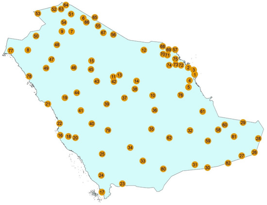
Figure 1.
Distribution of the 82 selected sites in Saudi Arabia. The numbers in the circles refer to those in column 1 of Table 1.
2.2. Data Processing and Analysis
In step 1, the downloaded hourly data from the PV-GIS website were transferred from the coordinated universal time (UTC) into the Saudi Arabia local standard one (LST = UTC + 3 h). It must be mentioned here that the PV-GIS solar radiation values were provided at different UTC times for the various sites considered, e.g., at hh:48 or hh:09, where hh stands for any hour between 00 and 23. In step 2, the hourly global horizontal radiation, Hg,0, values were estimated as the sum Hg,0 = Hb,0 + Hd,0. In step 3, the original Sun’s azimuth and elevation (SUNAE) routine introduced by Walraven [36], together with its modifications [37,38,39,40] renaming SUNAE to XRONOS (meaning time in Greek, X is pronounced CH), ran for the geographical coordinates of the 82 sites in the period 2005–2016 to derive the solar altitudes, γ; the XRONOS algorithm computed γ at the LST times so calculated in step 1. In step 4, all radiation and solar geometry values were assigned to the nearest LST hour (i.e., values at hh:48 LST or hh:09 LST were assigned to just hh:00 LST). That was done in order to have all values in the data base at integer hours. In the next step 5, only those hourly solar radiation values were retained for analysis that were greater than 0 Wm−2, and for γ ≥ 5° (to avoid the cosine effect). Also, the criterion of Hd,0 ≤ Hg,0 should be met at hourly level.
For estimating global solar irradiance on an inclined plane facing south, Hg,βS (in Wm−2), the isotropic model of Liu-Jordan [41] was adopted (β is the tilt angle of the inclined plane in respect to the local horizon, in degrees). The isotropic model was used to estimate the ground-reflected radiation from the surrounding surface, Hr,βS (in Wm−2), received on the inclined flat surface. This model has been adopted in the present study because it has proved as efficient in providing the tilted total solar radiation in many parts of the world as other more sophisticated models [42]. For a south-facing surface the received total solar radiation is given by [43]:
where the subscript S denotes the south orientation of the inclined surface. According to Liu-Jordan [41]:
where θ is the incidence angle (the angle formed by the normal to the inclined surface and the line joining the surface with the centre of the Sun), and ψ, ψ’ are the solar azimuths of the Sun and of the inclined plane, respectively; the latter two solar parameters were estimated through the XRONOS algorithm, while ψ’ was always equal to 180 degrees to south. The parameters Rdi and Rr are called the isotropic sky-configuration and ground-inclined plane-configuration factors, respectively. In the Liu-Jordan model the ground albedo usually takes the value of ρg0 = 0.2 (Equation (3)). This value has also been used in the present study. Apart from using ρg0 in the calculations, values of ρg near to reality were also adopted and used here. To retrieve such values for the 82 sites, use of the Giovanni portal [44] was made; pixels of 0.5° × 0.625° spatial resolution were centered over each of the 82 sites for which monthly mean values of the ground albedo were downloaded in the period of the study (2005–2016); annual mean ρg values were then computed and were used to re-calculate Hg,βS.
Hg,βS = Hb,βS + Hd,βS + Hr,βS,
Hd,βS = Hd,0·Rdi,
Hr,βS = Hg,0·Rr·ρg0, (or ρg)
Rdi = (1 + cosβ)/2,
Rr = (1 − cosβ)/2,
Hb,βS = Hb,0·cosθ/sinγ,
cosθ = sinβ·cosγ·cos(ψ − ψ’) + cosβ·sinγ.
In the present study, β varied in the range 15°–55° in increment of 5°; this range was chosen so that it fully covers all latitudes of Saudi Arabia (from ≈18° N to 32° N). For every site and tilt angle, hourly values of Hg,βS were estimated twice from Equation (1); the first time the computations included ρg0 = 0.2, and the second time the calculations were repeated with ρg (=ground-albedo value from Giovanni). From the hourly Hg,βS values, annual, seasonal and monthly solar energy sums (in kWhm−2) under all-sky conditions were estimated for all sites, all tilt angles and both ground-albedo values.
3. Results
3.1. Annual Energy Sums and Solar Energy Zones
Table 2 shows the maximum annual Hg,opt. βS sums for all sites with their corresponding tilt angles, β. The derivation of those energy values was based on the optimum angle β (in the range 15°–55° in steps of 5°) for which maximum Hg,βS was obtained. Along with each maximum Hg,opt. βS the corresponding optimum β is shown. Differences of the annual energy sums, ΔHg,βS, were then derived through using ρg and ρg0 in Equation (3), i.e., ΔHg,βS = Hg,βS/ρg. − Hg,βS/ρg0. Note that the optimum βs differ between the two cases (columns 2 and 3 in Table 2, respectively). The truth is that the reference value of ρg0 is applicable to grassland areas; surfaces with different vegetation or no vegetation (e.g., tundras, deserts, snow-covered areas) may have reflectance far from 0.2 [42]. The differences ΔHg,βS are shown in Figure 2 for all 82 sites. From these Figs. it is seen that almost all differences are positive. This occurs for the sites having ρg > ρg0, i.e., for a ground albedo greater than 0.2; the negative differences correspond to sites having ρg < ρg0, i.e., for a ground albedo less than 0.2. It is considered that the Hg,opt. βS/ρg values are closer to reality because of the use of the near-real ground-albedo values ρg; therefore, the present study deals with these “pragmatic” annual solar energy sums in the rest of the analysis. Figure 3 shows the distribution of ρg over Saudi Arabia.
Table 2.
Maximum Hg,opt. βS annual sums for the 82 sites in Saudi Arabia for optimally-selected tilt angles, opt. β, towards south (S) derived by using a ground albedo of ρg0 = 0.2 and of actual ρg., under all-sky conditions in the period 2005–2016.
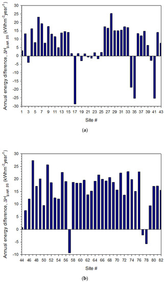
Figure 2.
(a) Differences of annual maximum solar energy sums, ΔHg,opt. βS, on flat planes with optimally-derived tilt angles Figure 1. and (b) 44–82, under all-sky conditions and averaged over the period 2005–2016. ΔHg,opt. βS = Hg,opt. βS/ρg. − Hg,opt. βS/ρg0, where opt. β refers to the angles shown in Table 2 for both ground-albedo cases of ρg and ρg0.
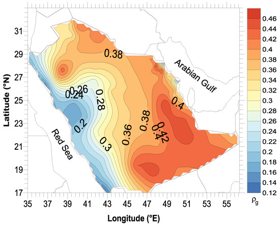
Figure 3.
Distribution of the annual mean ground-albedo, ρg, values over Saudi Arabia in the period 2005–2016. The x-axis is the geographical longitude, λ, and the y-axis is the geographical latitude, φ (both in degrees).
Considering the maximum energy sums and optimal tilt angles given in column 3 of Table 2, a new map was derived in Figure 4, where the 82 sites are shown in different colours and symbols; the sites are grouped according to the same optimum β. It is apparent that 3 distinct solar energy zones (SEZ) are formed: (i) SEZ-A (red circles) with optimum β = 20° S, (ii) SEZ-B (orange circles) with optimum β = 25° S, and (iii) SEZ-C (green circles) with optimum β = 30° S. Contrary to this result, Zell et al. [27] divided the country into 5 geographical regions (central, eastern, southern, western, western inland) for the purpose of analysing the solar radiation data from [45]. Nevertheless, the division of Zell et al.’s did not obey any solar radiation criteria, while the SEZs in the present work really meet the mentioned energy criteria; therefore, it is of no practical value.
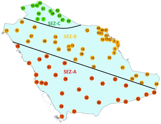
Figure 4.
Distribution of the 82 sites in different colours and symbols: red circles refer to sites with optimum β = 20° S (SEZ-A), orange circles to sites with optimum β = 25° S (SEZ-B), and green circles to sites with optimum β = 30° S (SEZ-C). The numbers in the symbols refer to the sites (column 1, Table 2).
Kaddoura et al. [23] estimated 12 optimal angles β for the 12 months of the year for Tabuk (#8 in Table 1), Al Jawf (#9), Riyadh (#10), Jeddah (#16), and Abha (#24). These angles were derived from modelling and they, therefore, have a purely theoretical value, since it is not practical at all to change the tilt angle of the solar panel frame every month. To the contrary, the present work gives a constant tilt angle throughout the year at any site in Saudi Arabia belonging to the same SEZ. Zell et al. [27] calculated average annual values for the optimal tilt angles of 25.6°, 26.4°, 19.4°, 19.3°, and 16.5° for the mentioned cities in [23], respectively. The tilt angles from the present study (Table 2) are 25°, 30°, 25°, 20°, and 20°, respectively, which are very close to the average values of [27]. El-Sebaii et al. [26] agree with the optimum tilt angle for Jeddah as they find it to be 21.76°, close to the 20° of this study.
3.2. Monthly Energy Sums
The intra-annual variation of Hg,opt. βS/ρg in each specific SEZ region is shown in Figure 5. Figure 5a refers to the sites in SEZ-A (optimal β = 20°), Figure 5b to the sites in SEZ-B (optimal β = 25°), and Figure 5c to the sites in SEZ-C (optimal β = 30°). The expressions for the lines that best-fit the means and their coefficient of determination, R2, are given in Table 3. It is seen that the R2 statistic obtains high values; this allows a solar energy user or investor in Saudi Arabia to estimate the monthly energy production in any of the 3 SEZs in an accurate way by applying the regression equations. The graphs also contain curves for the mean ± 1 standard deviation (σ).
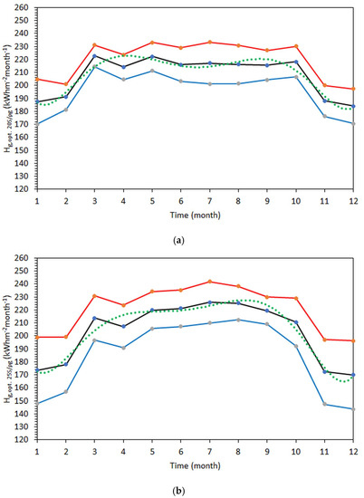
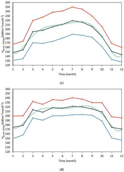
Figure 5.
Intra-annual variation of (a) Hg,opt. 20S/ρg in SEZ-A, (b) Hg,opt. 25S/ρg in SEZ-B, (c) Hg,opt. 30S/ρg in SEZ-C, and (d) Hg,opt. βS/ρg in all SEZs, under all-sky conditions and averaged over the period 2005–2016. The black solid lines represent the monthly Hg sums averaged over all corresponding sites. The red lines correspond to the mean + 1σ curves, and the blue lines to the mean − 1σ curves. The green dotted lines refer to the best-fit curves to the mean ones.
Table 3.
Regression equations for the best-fit curves to the monthly/seasonal mean Hg,βS/ρg sums averaged over all respective sites in the period 2005–2016, together with their R2 values; t is either month in the range 1–12 or season in the range 1–4 (1 = spring, 2 = summer, 3 = autumn, 4 = winter).
3.3. Seasonal Energy Sums
Investors in solar energy installations are mostly interested in knowing the minimum and maximum possible energy received by their energy systems. This is interpreted as the solar potential during the winter and summer months. Therefore, this Section is devoted to analysing the solar energy totals during all seasons, i.e., spring (March-April-May), summer (June-July-August), autumn (September-October-November) and winter (December-January-February).
Figure 6 presents the total solar energy received on a south-oriented flat surface in SEZ-A (Figure 6a), SEZ-B (Figure 6b), SEZ-C (Figure 6c), and all SEZs (Figure 6d) under all-sky conditions during spring, summer, autumn, and winter. The energy values are sums for each season averaged over all sites belonging to the same SEZ (or all SEZs). Table 3 gives the regression equations for the curves that best fit the mean ones in each case. It is interesting to observe that the fits are ideal (R2 = 1) in all cases.
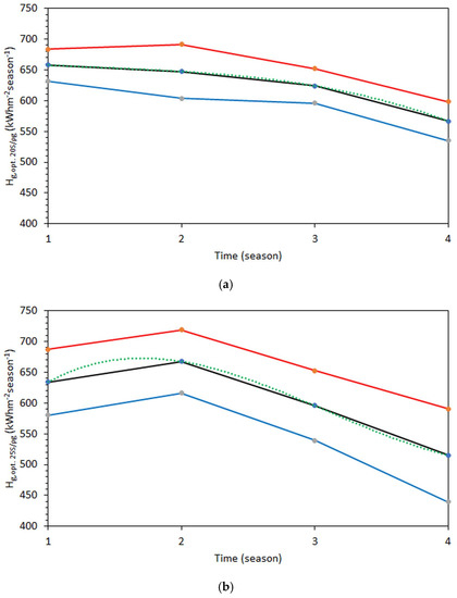
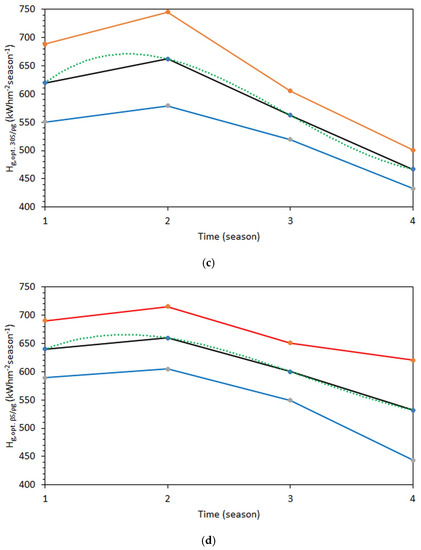
Figure 6.
Seasonal variation of (a) Hg,opt. 20S/ρg in SEZ-A, (b) Hg,opt. 25S/ρg in SEZ-B, (c) Hg,opt. 30S/ρg in SEZ-C, and (d) Hg,opt. βS/ρg in all Scheme 1. curves, and the blue lines to the mean − 1σ curves, under all-sky conditions and averaged over the period 2005–2016. The green dotted lines refer to the best-fit curves to the mean ones. The numbers 1–4 in the x-axis refer to the seasons in the sequence spring to winter.
3.4. Maps of Annual Energy Sums
Figure 7 shows the solar potential over Saudi Arabia in terms of annual Hg,0 and Hg,opt. βS/ρg sums. It is interesting to observe a gradual increase in the annual solar potential in the direction NE–SW for both horizontal and optimally inclined flat planes. Very similar results to the present study are given in the Solar Radiation Atlas for Saudi Arabia [45]. This gradient is due to two reasons. (i) Latitude: the higher the latitude, the less solar radiation is received on the surface of the Earth. (ii) Meteorology: more frequent precipitation is observed in the north-eastern part of the country, which is related to the precipitation occurring in southern Iraq and Iran [46].
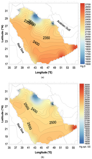
Figure 7.
Distribution of the annual (a) Hg,0 (kWhm−2year−1) and (b) Hg,opt. βS/ρg (kWhm−2year−1) sums over Saudi Arabia, under all-sky conditions and averaged over the period 2005–2016. The x-axis is the geographical longitude, λ (in degrees east), and the y-axis the geographical latitude, φ (in degrees north).
3.5. Evaluation of the PV-GIS Tool
Given that all data used in this study were downloaded from the PV-GIS platform, the question arises as to the accuracy and reliability of these data. For this reason, various studies have presented validation results for the solar radiation PV-GIS-satellite-derived data by comparing them with ground-based solar radiation measurements from 30 BSRN stations [30,34,35]. The reported % differences in the form of “100*(PV-GIS-data—station-data)/station-data” were found to vary between −14% to +11%. To further demonstrate this, comparison of monthly mean Hg,0 values derived from solar radiation measurements continuously performed at the Actinometric Station of the National Observatory of Athens (ASNOA, 37.97° N, 23.72° E, 107 m above sea level) was made with respective values from the PV-GIS platform in the period 2005–2011. The ASNOA site was selected as Saudi Arabia does not possess any permanent solar radiation measuring network nor isolated measuring radiometric stations on a systematic basis. The only station that participated in many international networks (e.g., AERONET, BSRN) is the Solar Village one (18.23° N, 42.66° E, 2039 m above sea level) that was in operation during the period March 1998–December 2002, a period that does not include the starting date of PV-GIS (January 2005). Figure 8 shows this comparison. Although there is an excellent agreement qualitatively (R2 = 0.99), it seems that the PV-GIS-retrieved data overestimate the measured Hg,0 by a factor of 1.1; this ratio is defined by any Hg,0 value on the best-fit line to the corresponding one on the 1:1 line. In other words, the PV-GIS data are +10% higher than the ASNOA values, in accordance to the error range mentioned above. Nevertheless, as this factor is small and R2 is high, the PV-GIS data are considered acceptable for solar energy analyses.
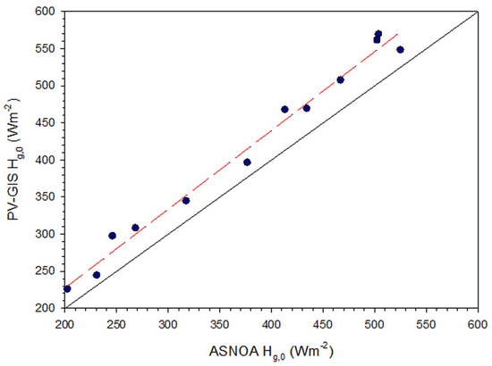
Figure 8.
Comparison of monthly mean Hg,0 values from PV-GIS to measured Hg,0 values at ASNOA in the period 2005–2011. The red dashed line represents the best fit to the data points and is expressed by the regression equation: PV-GIS Hg,0 = 1.06·ASNOA Hg,0 + 14.96 (R2 = 0.99). The solid black line is the 1:1 (or y = x) line.
3.6. Definition and Variation of the Correction Factor
This Section uses the notion of the correction factor, CF. This factor is defined by: CF = Hg,opt. βS/ρg/Hg,opt. βS/ρg0. In other words, CF is the ratio of the annual Hg,βS sum at each site of the 82, calculated twice, once for ρg0 = 0.2 and a second time for ρg = actual value; β is the tilt angle in the range 15°–55°. CF is named correction factor because it renders the maximum annual solar energy sum on a flat plane at a site in Saudi Arabia inclined to the south under the influence of the real terrain surrounding the location if this energy maximum value is known for an albedo value of 0.2. In other words, CF corrects the energy on an inclined surface under the influence of a ground albedo equal to 0.2 to that which is under the influence of near-real ground-albedo value. Figure 9 presents the variation of CF as function of β for all 82 sites; the controlling parameter is the ratio ρr = ρg/ρg0, which takes a different value at each site. It is seen that the higher the ρr value is, the more concave the best-fit curve is (for CF > 1); to the contrary, the lower the ρr value is, the more convex the best-fit curve becomes (for CF < 1). All the data points at every β correspond to the 82 sites. The distribution of ρr at the 82 sites is shown in Figure 10.
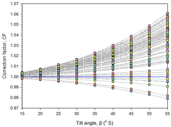
Figure 9.
Variation of the correction factor, CF, as function of the tilt angle of the inclined flat plane, β, towards south (S), under all-sky conditions and averaged over the period 2005–2016. The blue straight line represents CF = 1; site #24 is very close to this value (0.98, Figure 10a). The dotted lines are the best-fit curves to the data points of each site. The best-fit lines are expressed by 3rd-order polynomials. For example, the upper best-fit curve is: CF = 2·10−7 β3 + 5·10−6 β2 + 1·10−4 β + 0.9977 (R2 = 1), while the lowest one: CF = −5·10−8 β3 − 2·10−6 β2 − 9·10−5 β + 1.0006 (R2 = 1). The blue horizontal line indicates CF = 1.
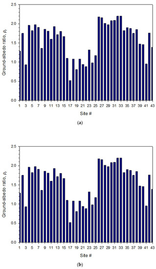
Figure 10.
Annual mean ratios of ground albedo, ρr, for the 82 sites in Saudi Arabia; (a) sites 1–43, (b) sites 44–82, averaged over the period 2005–2016.
Further, a diagram of CF vs. ρr is shown in Figure 11, where a linear relationship is revealed and is shown for all sites. The controlling parameter in this case is β; as β increases, the slope of the linear fit to the data points decreases. The data points along each line correspond to the 82 sites.
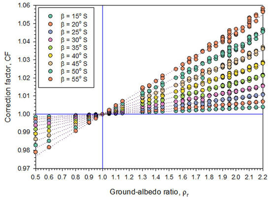
Figure 11.
Variation of the correction factor, CF, as function of the ground-albedo ratio, ρr, for various tilt angles, β, for a flat plane in Saudi Arabia inclined towards south (S), averaged over the period 2005–2016. The blue lines correspond to ρr = 1 and CF =1.
Despite the above, a more detailed analysis was performed for the function CF. In this analysis, the average values of CF were calculated for all βs and all sites belonging to the same SEZ, as well as all sites irrespective of SEZ. The results are shown in Figure 12, where the variation of CF with β in the range 15°–55° is shown. More particularly, the graphs give the variation of CF in a specific SEZ having the same optimum β, if the optimum tilt angle includes all values in the above range, i.e., if all βs become optimum in a specific SEZ. Table 4 gives the regression equations for the lines that best fit the data points in each SEZ and all SEZs too. These regression relationships have the same shape as those in Figure 9.
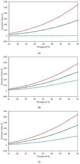
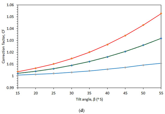
Figure 12.
Variation of the correction factor, CF, as function of the tilt angle, β, of an inclined surface towards south (S) in (a) SEZ-A, (b) SEZ-B, (c) SEZ-C, and (d) all SEZs, averaged over the period 2005–2016. The black solid lines are the mean CF values, while the red and blue ones correspond to the mean + 1σ, and mean − 1σ, respectively. The green dotted lines are the best fits to the mean curves and are hardly seen as they coincide with the mean curves.
Table 4.
Regression equations for the best-fit curves to the correction-factor, CF, values averaged over all respective sites in the period 2005–2016, together with their R2 values; β is the optimum tilt angle of a flat surface inclined in a SEZ towards south (S).
4. Conclusions and Discussion
The present study investigated the solar availability across Saudi Arabia on flat-plate solar panels with south orientation. The main objective was to find the optimum tilt angles of solar panels that produce maximum annual energy under all-sky conditions. This was achieved by calculating the annual energy sum on flat-plate surfaces with tilt angles in the range 5°–55° towards south with an increment of 5° at 82 sites across Saudi Arabia; the solar availability on a horizontal plane was also included. The calculations of the energy received on the tilted surfaces were repeated for both a ground albedo equal to 0.2 (reference value) and a near-real ground albedo.
The first outcome of the work was that the optimum tilt angles over Saudi Arabia are 20°, 25°, and 30° towards south. The second finding of the study was that these 3 optimum tilt angles group the 82 sites into 3 (solar energy) zones (SEZ), i.e., SEZ-A with 20° S, SEZ-B with 25° S, and SEZ-C with 30° S. The third conclusion was related with the variation of the annual maximum solar energy in each SEZ, i.e., 2192–2595 kWhm−2year−1 (SEZ-A), 1612–2977 kWhm−2year−1 (SEZ-B), 1702–2587 kWhm−2year−1 (SEZ-C), and 1612–2977 kWhm−2year−1 (all SEZs). Beside the annual energy sums, monthly solar energy ones averaged over all locations belonging to the same SEZ as well as to all SEZs were estimated under all-sky conditions. Regression equations were provided as best-fit curves to the monthly mean energy sums that estimate the solar energy potential per SEZ (and all SEZs) with great accuracy (R2 ≥ 0.90). These expressions may prove very useful to architects, civil engineers, solar energy engineers, and solar energy-systems investors in order to assess the solar energy availability in Saudi Arabia throughout the year.
Seasonal solar energy sums were also calculated. They were averaged over all sites in the same SEZ as well over all sites (all SEZs) as in the case of the annual and monthly sums, under all-sky conditions. For every case, regression curves that best fit the mean values were estimated with greatest accuracy (R2 = 1). Maximum sums were found in the summer (730 kWm−2), and minimum ones in the winter (450 kWm−2), as expected.
A correction factor, CF, was defined as the ratio of the maximum solar energy sum derived from calculations with near-real ground albedos, ρg, to that derived with the reference value, ρ0. A graph of CF as function of the tilt angle (in the range 15°–55°) showed an exponential growth for sites having ratios ρg/ρ0 > 1, or an exponential decay in the cases of ρg/ρ0 < 1. Such curves are assumed to be universal (nomograms), but this remains to be proved for other locations in the world with different climate and terrain characteristics. Graph of CF as function of ρg/ρ0 was prepared for different values of the tilt angle (in the range 15°–55°). Best-fit lines to the data points were estimated and found to be linear of decreasing slope with decreasing tilt angle. These curves are also assumed to be nomograms, but this also has to be proved for other locations in the world with different climate and terrain characteristics.
Three innovations appeared in the present study: (i) For the first time, solar maps for Saudi Arabia of the maximum energy received on optimally-inclined flat surfaces towards south were derived; (ii) for the first time, three energy zones were identified in Saudi Arabia for solar applications; (iii) universal curves (nomograms) of CF in relation to the tilt angle and ρg/ρ0 were derived.
Based on the adopted methodology, some guidelines can be given here to interested solar energy scientists and/or solar energy entrepreneurs for applying them in their territory. If a solar radiation station exists in the area, hourly or daily values of the solar global horizontal radiation must be collected for a climatological period of 10 years at least. If no solar radiation exists, then data from a relative website (e.g., BSRN, GEBA, PV-GIS, ARM) can be obtained. In the extreme case that this option is not possible, use of a solar energy model can be made to derive the anticipated data from other available variables (e.g., meteorological parameters). Then, transposition of the selected data from horizontal to inclined planes towards the local south must take place by varying the tilt angles in a range that includes the geographical latitude of the site. In the next step, the annual solar energy sums on the inclined planes have to be calculated and the highest energy sum must be selected; then the corresponding tilt angle is the optimum for the site. The transposition can be achieved by selecting the wishful model (the L-J model is sufficient). It is recommended that a near-real ground albedo value is used in these calculations; if knowledge of this value is not available for the site, use of the nomogram of Figure 11 can be made to correct the solar energy sums by selecting the appropriate tilt angle. Finally, monthly solar energy sums can be estimated and regression lines be derived that can be used as guidelines for estimating the expected solar energy on flat planes with the selected tilt angle.
As far as the significance of the results of the present study is concerned in the solar industry and the society of Saudi Arabia, this can be summarized in the following. The solar industry has now a rule for the inclined parts of the solar system-support frames; the inclined surfaces of the supporting frames must have angles of 20°, 25° or 30° depending on the SEZ to be installed. It is assumed that the orientation of the supporting frame has to be towards south. This rule may reduce installation costs because of the standardisation of the supporting frame. On the other hand, the society may get indirect benefits from governmental initiatives regarding policies that promote renewable energy sources in Saudi Arabia (and especially solar energy sources) because of the new knowledge gained through the present work.
Author Contributions
Data collection, data analysis, writing—review and editing, A.F.; conceptualisation, methodology, data collection, data analysis, writing—original draft preparation, H.D.K.; writing—review and editing, E.R.; writing—review and editing, M.A. All authors have read and agreed to the published version of the manuscript.
Funding
Researchers would like to acknowledge the support provided by the Deanship of Scientific Research (DSR) at the King Fahd University of Petroleum and Minerals (KFUPM) for funding this work through project no. DF181010.
Institutional Review Board Statement
Not applicable.
Informed Consent Statement
Not applicable.
Data Availability Statement
The solar radiation data and the ground-albedo ones for Saudi Arabia are publicly available and were downloaded from the PV-GIS platform (https://ec.europa.eu/jrc/en/pvgis) and the Giovanni website (https://giovanni.gsfc.nasa.gov/giovanni/), respectively. The ASNOA solar radiation data are available on request, but they were used on a self-evident permission to the second author as ex. member and now Emeritus Researcher in the Institution.
Acknowledgments
The authors are thankful to the Giovanni-platform staff as well the MODIS-mission scientists and associated NASA personnel for the production of the ground-albedo data used in this research. They also thank the personnel of the PV-GIS platform for providing the necessary solar horizontal irradiances over Saudi Arabia. B.E. Psiloglou and N. Kappos are acknowledged for maintaining the solar radiation equipment on the ASNOA platform.
Conflicts of Interest
The authors declare no conflict of interest.
References
- Kambezidis, H.D. Annual and seasonal trends of solar radiation in Athens, Greece. J. Sol. Energy Res. Updates 2018, 5, 14–24. [Google Scholar] [CrossRef]
- Kambezidis, H.D. The solar radiation climate of Athens: Variations and tendencies in the period 1992–2017, the brightening era. Sol. Energy 2018, 173, 328–347. [Google Scholar] [CrossRef]
- Kambezidis, H.D. The solar resource. In Comprehensive Renewable Energy; Sayigh, A., Ed.; Elsevier: Amsterdam, The Netherlands, 2012; pp. 27–83. ISBN 978-0-08087-872-0. [Google Scholar]
- Hafez, A.Z.; Soliman, A.; El-Metwally, K.A.; Ismail, I.M. Tilt and azimuth angles in solar energy applications—A review. Renew. Sustain. Energy Rev. 2017, 77, 147–168. [Google Scholar] [CrossRef]
- Willmott, C.J. On the climatic optimization of the tilt and azimuth of flat-plate solar collectors. Sol. Energy 1982, 28, 205–216. [Google Scholar] [CrossRef]
- Rowlands, I.H.; Kemery, B.P.; Beausoleil-Morrison, I. Optimal solar-PV tilt angle and azimuth: An Ontario (Canada) case-study. Energy Policy 2011, 39, 1397–1409. [Google Scholar] [CrossRef]
- Daut, I.; Irwanto, M.; Irwan, Y.M.; Gomesh, N.; Ahmad, N.S. Clear sky global solar irradiance on tilt angles of photovoltaic module in Perlis, Northern Malaysia. In Proceedings of the International Conference on Electrical, Control and Computer Engineering (INECCE), Kuantan, Malaysia, 21–22 June 2011; pp. 445–450. [Google Scholar] [CrossRef]
- Khatib, T.; Mohamed, A.; Sopian, K. On the monthly optimum tilt angle of solar panel for five sites in Malaysia. In Proceedings of the IEEE International Power Engineering and Optimization Conference (PEDCO), Melaka, Malaysia, 6–7 June 2012; pp. 7–10. [Google Scholar] [CrossRef]
- Elhab, B.R.; Sopian, K.; Mat, S.; Lim, C.; Sulaiman, M.Y.; Ruslan, M.H.; Saadatian, O. Optimizing tilt angles and orientations of solar panels for Kuala Lumpur, Malaysia. Sci. Res. Essays 2012, 7, 3758–3765. [Google Scholar] [CrossRef]
- Altarawneh, I.S.; Rawadieh, S.I.; Tarawneh, M.S.; Alsowwad, S.M.; Ramawi, F. Optimal tilt angle trajectory for maximizing solar energy potential in Ma’an area, Jordan. J. Renew. Sustain. Energy 2016, 8, 033701. [Google Scholar] [CrossRef]
- Talebizadeh, P.; Mehrabian, M.A.; Abdolzadeh, M. Prediction of the optimum slope and surface azimuth angles using the Genetic Algorithm. Energy Build. 2011, 43, 2998–3005. [Google Scholar] [CrossRef]
- Jafarkazemi, F.; Saadabadi, S.A.; Pasdarshahri, H. The optimum tilt angle for flat-plate solar collectors in Iran. J. Renew. Sustain. Energy 2012, 4, 013118. [Google Scholar] [CrossRef]
- Kacira, M.; Simsek, M.; Babur, Y.; Demirkol, S. Determining optimum tilt angles and orientations of photovoltaic panels in Sanliurfa, Turkey. Renew. Energy 2004, 29, 1265–1275. [Google Scholar] [CrossRef]
- Skeiker, K. Optimum tilt angle and orientation for solar collectors in Syria. Energy Convers. Manag. 2009, 50, 2439–2448. [Google Scholar] [CrossRef]
- Ibrahim, D. Optimum tilt angle for solar collectors used in Cyprus. Renew. Energy 1995, 6, 813–819. [Google Scholar] [CrossRef]
- Ghosh, H.R.; Bhowmik, N.C.; Hussain, M. Determining seasonal optimum tilt angles, solar radiations on variously oriented, single and double axis tracking surfaces at Dhaka. Renew. Energy 2010, 35, 1292–1297. [Google Scholar] [CrossRef]
- Vasiliev, M.; Nur-E-Alam, M.; Alameh, K. recent technologies in solar energy-harvesting technologies for building integration and distributed energy generation. Energies 2019, 12, 1080. [Google Scholar] [CrossRef]
- Islam, M.T.; Huda, N.; Abdullah, A.B.; Saidur, R. A comprehensive review of state-of-the-art concentrating solar power (CSP) technologies: Current status and research trends. Renew. Sustain. Energy Rev. 2018, 91, 987–1018. [Google Scholar] [CrossRef]
- Ahmadi, H.M.; Ghazvini, M.; Sadeghzadeh, M.; Nazari, M.A.; Kumar, R.; Naeimi, A.; Ming, T. Solar power technology for electricity generation: A critical review. Energy Sci. Eng. 2018, 6, 340–361. [Google Scholar] [CrossRef]
- Vinod; Kumar, R.; Singh, S.K. Solar photovoltaic modeling and simulation: As a renewable energy solution. Energy Rep. 2018, 4, 701–712. [Google Scholar] [CrossRef]
- Bayrak, F.; Ertürk, G.; Oztop, H.F. Effects of partial shading on energy and exergy efficiencies for photovoltaic panels. J. Clean. Prod. 2017, 164, 58–69. [Google Scholar] [CrossRef]
- Evseev, E.G.; Kudish, A.I. The assessment of different models to predict the solar radiation on a surface tilted to the south. Sol. Energy 2009, 83, 377–388. [Google Scholar] [CrossRef]
- Kaddoura, T.O.; Ramli, M.A.M.; Al-Turki, Y.A. On the estimation of the optimum tilt angle of PV panel in Saudi Arabia. Renew. Sustain. Energy Rev. 2016, 65, 626–634. [Google Scholar] [CrossRef]
- Ohtake, H.; Uno, F.; Oozeki, T.; Yamada, Y.; Takenaka, H.; Nakajima, T.Y. Estimation of satellite-derived regional photovoltaic power generation using satellite-estimated solar radiation data. Energy Sci. Eng. 2018, 6, 570–583. [Google Scholar] [CrossRef]
- Kambezidis, H.D.; Psiloglou, B.E. Estimation of the optimum energy received by solar energy flat-plate convectors in Greece using Typical Meteorological Years. Part I: South-oriented tilt angles. Appl. Sci. 2021, 11, 1547. [Google Scholar] [CrossRef]
- El-Sebaii, A.A.; Al-Hazmi, F.S.; Al-Ghamdi, A.A.; Yaghmour, S.J. Global, direct and diffuse solar radiation on horizontal and tilted surfaces in Jeddah, Saudi Arabia. Appl. Energy 2010, 87, 568–576. [Google Scholar] [CrossRef]
- Zell, E.; Gasim, S.; Wilcox, S.; Katamoura, S.; Stoffel, T.; Shibli, H.; Engel-Cox, J.; Al Subie, M. Assessment of solar radiation resources in Saudi Arabia. Sol. Energy 2015, 119, 422–438. [Google Scholar] [CrossRef]
- The World Bank. Global Solar Atlas 2.0. 2019. Available online: https://solargis.com (accessed on 8 March 2021).
- Almasoud, A.H.; Gandayah, H.M. Future of solar energy in Saudi Arabia. J. King Saud Univ. Eng. Sci. 2015, 27, 153–157. [Google Scholar] [CrossRef]
- Müller, R.; Behrendt, T.; Hammer, A.; Kemper, A. A new algorithm for the satellite-based retrieval of solar surface irradiance in spectral bands. Remote Sens. 2012, 4, 622–647. [Google Scholar] [CrossRef]
- Huld, T.; Müller, R.; Gambardella, A. A new solar radiation database for estimating PV performance in Europe and Africa. Sol. Energy 2012, 86, 1803–1815. [Google Scholar] [CrossRef]
- Urraca, R.; Gracia Amillo, A.M.; Koubli, E.; Huld, T.; Trentmann, J.; Riihelä, A.; Lindfors, A.V.; Palmer, D.; Gottschalg, R.; Antonanzas-Torres, F. Extensive validation of CM SAF surface radiation products over Europe. Remote Sens. Environ. 2017, 199, 171–186. [Google Scholar] [CrossRef]
- Urraca, R.; Huld, T.; Gracia Amillo, A.; Martinez-de-Pison, F.J.; Kaspar, F.; Sanz-Garcia, A. Evaluation of global horizontal irradiance estimates from ERA5 and COSMO-REA6 reanalyses using ground and satellite-based data. Sol. Energy 2018, 164, 339–354. [Google Scholar] [CrossRef]
- Müller, R.; Matsoukas, C.; Gratzki, A.; Behr, H.; Hollman, R. The CM-SAF operational scheme for the satellite-based retrieval of solar irradiance—A LUT based eigenvector hybrid approach. Remote Sens. Environ. 2009, 113, 1012–1024. [Google Scholar] [CrossRef]
- Gracia Amillo, A.; Huld, T.; Müeller, R. A new database of global and direct solar radiation using the eastern meteosat satellite, models and validation. Remote Sens. 2014, 6, 8165–8189. [Google Scholar] [CrossRef]
- Walraven, R. Calculating the position of the sun. Sol. Energy 1978, 20, 393–397. [Google Scholar] [CrossRef]
- Wilkinson, B.J. An improved FORTRAN program for the rapid calculation of the solar position. Sol. Energy 1981, 27, 67–68. [Google Scholar] [CrossRef]
- Muir, L.R. Comments on “The effect of the atmospheric refraction in the solar azimuth”. Sol. Energy 1983, 30, 295. [Google Scholar] [CrossRef]
- Kambezidis, H.D.; Papanikolaou, N.S. Solar position and atmospheric refraction. Sol. Energy 1990, 44, 143–144. [Google Scholar] [CrossRef]
- Kambezidis, H.D.; Tsangrassoulis, A.E. Solar position and right ascension. Sol. Energy 1993, 50, 415–416. [Google Scholar] [CrossRef]
- Liu, B.Y.H.; Jordan, R.C. The long-term average performance of flat-plate solar energy collectors. Sol. Energy 1963, 7, 53–74. [Google Scholar] [CrossRef]
- Kambezidis, H.D.; Psiloglou, B.E.; Gueymard, C.A. Measurements and models for total solar irradiance on inclined surface in Athens, Greece. Sol. Energy 1994, 53, 177–185. [Google Scholar] [CrossRef]
- Iqbal, M. An Introduction to Solar Radiation; Academic Press: Toronto, ON, Canada, 1983; pp. 304–307. ISBN 0-12-373750-8. [Google Scholar]
- Acker, J.G.; Leptoukh, G. Online analysis enhances use of NASA earth Science Data. EOS Trans. AGU 2007, 88, 14–17. [Google Scholar] [CrossRef]
- Solar Radiation Atlas for the Kingdom of Saudi Arabia. Prepared by the National Renewable Energy Laboratory (USA) and the Energy Institute (Saudi Arabia), November 1998. Available online: https://digital.library.unt.edu/ark:/67531/metadc690351/m2/1/high_res_d/5834 (accessed on 29 April 2021).
- Almazroui, M.; Islam, M.N.; Jones, P.D.; Athar, H.; Rahman, M.A. Recent climate change in the Arabian Peninsula: Seasonal rainfall and temperature climatology of Saudi Arabia for 1979–2009. Atmos. Res. 2012, 111, 29–45. [Google Scholar] [CrossRef]


Publisher’s Note: MDPI stays neutral with regard to jurisdictional claims in published maps and institutional affiliations. |
© 2021 by the authors. Licensee MDPI, Basel, Switzerland. This article is an open access article distributed under the terms and conditions of the Creative Commons Attribution (CC BY) license (https://creativecommons.org/licenses/by/4.0/).