Aerodynamic Response and Running Posture Analysis When the Train Passes a Crosswind Region on a Bridge

Abstract

Trains running on a bridge face more significant safety risks. Based on the Unsteady Reynolds-Averaged Navier–Stokes turbulence model, a three-dimensional Computational Fluid Dynamics computational model of the train–bridge–wind barrier was proposed in this study to measure the transient aerodynamic load of the train. The transient aerodynamic load was input into the wind–train–bridge coupling dynamic system to perform dynamic analysis of running safety. Significant fluctuations in the aerodynamic coefficients were found when the train entered and exited the wind barrier due to the dramatic change in flow pattern. The maximum value of the derailment coefficient decreased with the height of wind barriers, which hardly affected the wheel load reduction rate. The 2 m high wind barrier had no evident influence on the running posture of a general high-speed train, while the 4 m high wind barrier was proven to have better protection. Over-protection was found with an even higher wind barrier.

1. Introduction

Trains play an increasingly important role in passenger and freight transportation as a vehicle of high-speed and cost-effective public transportation. However, when there is a crosswind, the running train is subjected to an arbitrary speed limit, which has a major impact on carrying performance. The crosswind also poses a threat to operational safety [1]. As a result, train aerodynamic performance and operational protection in crosswinds have been extensively researched [2,3]. Because of their universality, trains that run on flat ground have gotten the most coverage [4]. Trains subjected to crosswinds in other common terrains have also been studied [5,6,7].

China is following a construction principle of “replace on-ground lines with bridges” due to topographic constraints, ground conditions, technical specifications of lines, land resources, and environmental protection. The majority of China’s high-speed railway lines are currently made up of bridges. In mountainous areas, high-speed rail lines are almost entirely made up of bridges and tunnels. The Beijing–Shanghai high-speed railway has 86.5 percent bridges, and the Shanghai–Hangzhou high-speed railway has even more, at 90 percent. According to the previous study [8], the trains on the bridges face a greater risk of overturning as the airflow rises with the height in the atmospheric boundary layers. This potential risk has brought a lot of research on the train passing the bridge [9,10].

Installing a windshield on the bridge can effectively protect the safety of train operation, as it was thought that a wind barrier could create a low-wind zone for vehicles, reducing the risk of strong wind [11]. The capacity of train windshields to protect passengers has been investigated using theoretical analysis, computational fluid dynamics, and full-scale and/or wind tunnel research [12,13]. Some influencing factors that affect the wind barrier’s efficiency were found: the barrier type, the height of the wind barrier, and the porosity. The porosity of the wind barrier and the vehicle’s position greatly impact the vehicle’s aerodynamic coefficients on the bridge floor. The aerodynamic coefficients of vehicles have been significantly reduced thanks to the wind barrier. Vehicles on the windward side of the bridge have higher aerodynamic coefficients than vehicles on the leeward side [14]. The aerodynamic forces of wind–vehicle–bridge systems were significantly affected by height and ventilation ratios, especially the side forces of the vehicles on the bridge deck. Furthermore, wind barriers significantly reduced aerodynamic vehicle forces while increasing bridge aerodynamic forces [15]. The sheltering output of a train above a railway bridge and the variation laws of flow field structure leeward a corrugated wind barrier with different bending angles were investigated, and the result showed that the lateral force and overturning moment of the barrier decreased as the bending angle increased, while there were no noticeable improvements in the lift force [16].

For most studies of windshield effects, static trains are used. Although such research methods have low computational cost and strong versatility for calculating the flow field around the train, they cannot simulate the train’s movement under the combined effect of the transient flow field and the crosswind. Given this, there are also some studies on trains dynamically crossing bridges. The wind–train–bridge coupling was studied using a dynamic analysis model. In the bridge-tunnel portion, the effects of a wind barrier with a height of 3 m and a porosity of 30% on the aerodynamic coefficient, flow field structure, and running protection of high-speed trains under crosswind were investigated. The wind barrier greatly reduced the sharp change effect of the aerodynamic coefficient by more than 50%, according to the results [17]. By constructing a wind–train–bridge dynamic coupled device, the train’s dynamic responses in the tunnel–bridge-tunnel infrastructure in the canyon wind environment, including displacement and acceleration parameters, wheel-rail response, and traffic safety indices, were investigated [5]. Deng discovered that when trains pass into a tunnel under crosswind, transient changes in the flow field structure and aerodynamic characteristics occur, reducing running safety [18].

Although these studies are focused on a dynamic model based on a moving train, most of them are concerned with the train’s transient degradation of aerodynamic performance as it passes through various surrounding scenes. However, the safety of the train operation rather than the aerodynamic performance of the train should be the ultimate concern. In addition, as previously described, the wind barrier plays a vital role during the operation of the train on the bridge, and the height of a wind barrier has a significant impact on its sheltering ability [19]. In different environments, wind barriers of different heights are used, and their effect on the dynamic running posture of the train is still unclear. For this consideration, a study on the height of the wind wall based on the dynamic analysis model of the wind–train–bridge coupling should be involved to evaluate its impact on the train’s dynamic performance and safe operation.

Based on the Unsteady Reynolds-Averaged Navier–Stokes (URANS) turbulence model, a three-dimensional (3D) Computational Fluid Dynamics (CFD) model of the train–bridge–wind barrier is proposed in this study to measure the transient aerodynamic load of the train. The transient aerodynamic load was fed into the wind–train–bridge coupling dynamic system to perform dynamic analysis of running safety. From the perspective of the train’s aerodynamic coefficient and flow field structure, the process and effect of the wind barrier height on the sudden change in aerodynamic performance of high-speed trains (HSTs) running on the bridge were investigated. Based on the changing characteristics of the train derailment coefficient (DC) and wheel load reduction rate (WLRR), the effect of wind barrier height and the running speed on running safety were addressed. The time-varying changes of the train’s running posture and acceleration in five degrees of freedom were also compared and analyzed. The CAD model, methodology, computational domain, boundary conditions, and meshes are discussed in Section 2, followed by a summary of the findings in Section 3, and finally a conclusion in Section 4.

2. Methodology

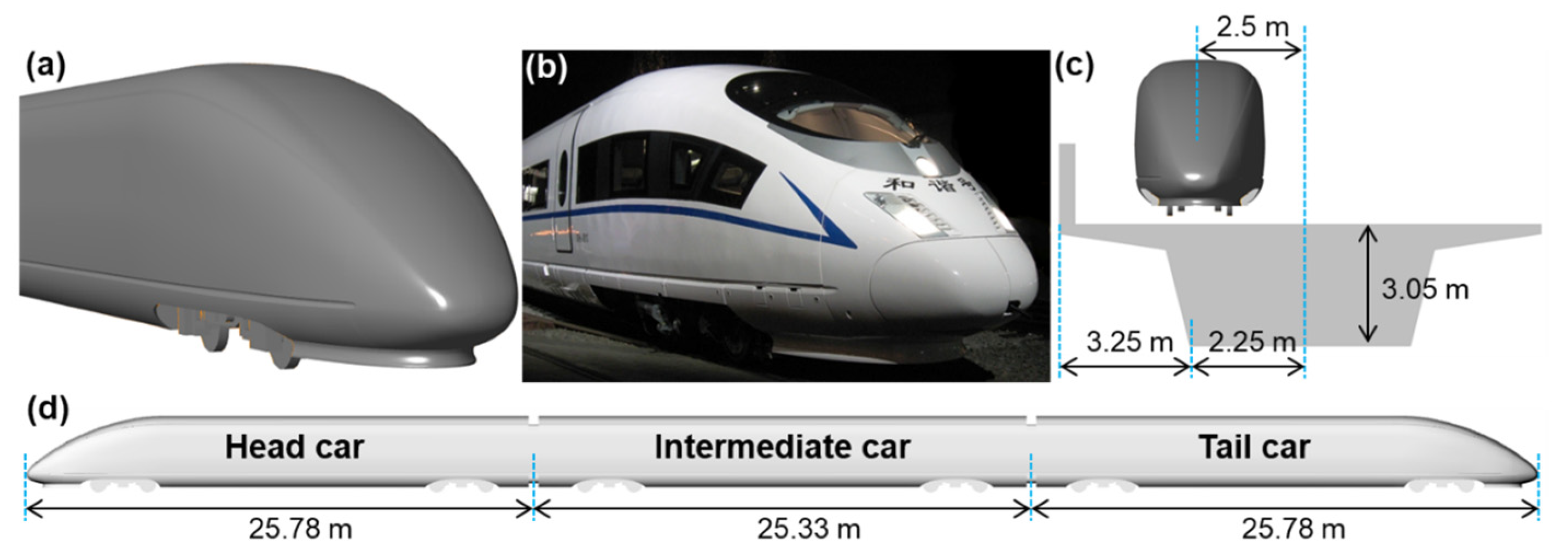
2.1. Model Description

As shown in Figure 1, the train used in the current study was the classic Chinese CRH3 high-speed train, which has the same scale as the real one. The train consisted of a head car, an intermediate car, and a tail car. Their lengths were 25.78 m, 25.33 m, and 25.78 m, respectively, which made the entire train 76.9 m long. The width and height of the train were 3.26 m and 3.89 m, respectively. To improve the efficiency of grid generation and numerical simulation, some geometric details on the train, such as doors, windows, handles, etc., were ignored, while geometric features that may potentially affect the dynamic response of the train, such as bogies and windshields, were preserved. The lowest end of the train (the lower vertex of the bogie wheelset) was 0.2 m away from the bridge deck to reproduce the ground clearance brought by the railway track.

The cross-section profile of the bridge was the 32 m simply supported box girder commonly used in Chinese high-speed railways, and the pier, track, and other ancillary structures were ignored. The distance between the two tracks was 5.0 m, and the train was located on the windward track, where the train has a greater risk of overturning, making the result more conservative. In this study, the train ran on a bridge with a length of 600 m, and only the middle 200 m was subjected to an ambient crosswind so that the transient performance of the aerodynamic performance of the train when passing through the crosswind area could be studied simultaneously. The wind barrier (if available) was installed upstream of the train to provide wind protection. Its width was 0.4 m, and its length was equal to that of the crosswind area.

2.2. Numerical Method

Various methods, such as Large Eddy Simulation (LES) and Detached Eddy Simulation (DES), show a major accuracy advantage in representing the precise shift inflow structures when simulating flow fields with large Reynolds numbers. However, as the mesh resolution and time-step become more stringent, computational efficiency suffers, and these methods are challenging to complete the work mentioned in this analysis. Furthermore, the Unsteady Reynolds-Averaged Navier–Stokes (URANS) equations turbulence model is commonly used in simulating flow structures similar to those in this analysis. As a result, in the present investigation, the 3D unsteady RNG k–ɛ turbulence model was used to simulate the flow field as HSTs travel through the bridge.

The STAR CCM+ 13.06 commercial software was used to perform the calculations. A pressure-based solver based on the finite volume method was used to obtain the pressure data. A second-order upwind scheme was applied to discretize the convection and diffusion concepts. An implied scheme with second-order accuracy was used to deal with the time term, and the time-step was set as 5 × 10⁻⁴ s was the physical time stage scale. Each time stage had 20 iterations, and the residual of each turbulent equation was at least 10 × 10⁻⁵ at each step.

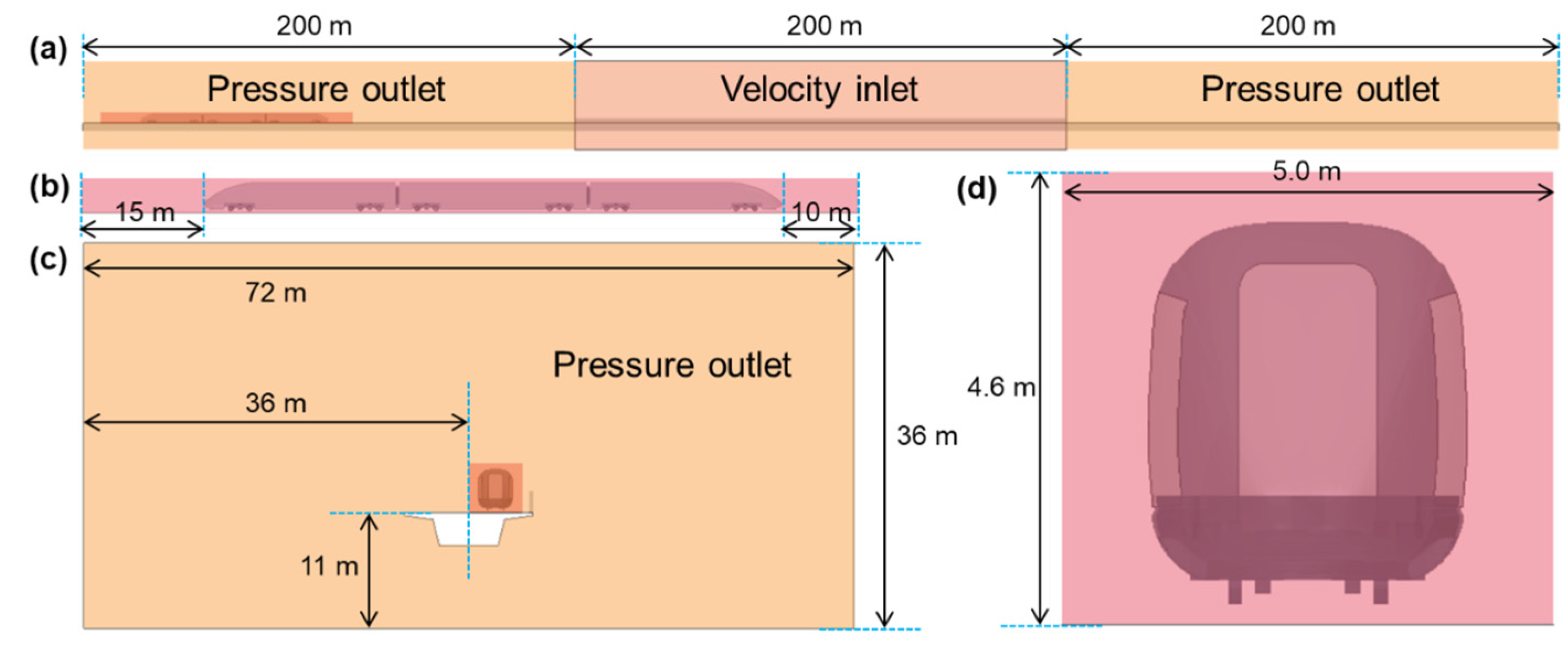
2.3. Computational Domain and Boundary Conditions

As shown in Figure 2, the entire calculation domain was 600 m long, 72 m wide, and 36 m high. The train was located in the middle of the width of the computational domain and was lower in the height direction. As described in Section 2.1, the entire computational domain could be divided into three sections in the length direction (shown in Figure 2a). Only the middle section of 200 m in length was filled with a crosswind given by a velocity inlet, and its speed $V_w$ was applied to a constant of 20 m/s. The other outer surfaces of the domain were all pressure outlets to replicate the reality. As shown in Figure 2b, an overset mesh was applied in current simulations to produce a relative motion of the train, bringing many more flexible mesh modifications during motion than the traditional meshing strategy. It had an independent grid distribution and exchanged real-time grid information with the background domain. The nose tip of the train head was 10 m away from the front end of this overset region, and the nose tip of the tail was 15 m away from another end, which ensured the flow development and stable information exchange between the two domains. This overset region had a total length of 102 m, a width of 5 m, and a height of 4.6 m, as shown in Figure 2d. The interfaces between the overset region and the larger domain were set to overset mesh boundary conditions, and the bottoms were set to the wall boundary. The distance from the train surface to the outer surfaces of the overset region allowed enough grid layers to be distributed in the space between the exchange surface and the train surface, making information exchange more reliable. The nose tip of the head of the train was initially located at a position 100 m away from the crosswind region and ends until the nose tip of the tail car reached 100 m out of the crosswind region, and the entire travel distance was 477 m. With a train speed $V_t$ of 300 km/h, the physical time for the simulation was 5.724 s.

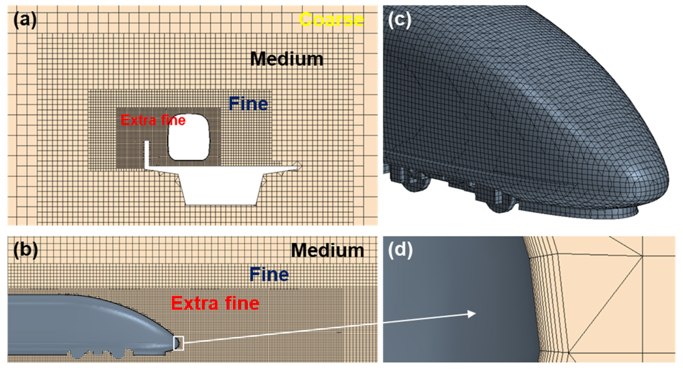
2.4. Meshing Strategy

In these simulations, the computational domains were discretized using the STAR CCM+ software’s unstructured hexahedral grids generator. Three different levels of refinement boxes were used for the transition from the grids at the domain’s outer surfaces to the train and bridge wall, as shown in Figure 3a,b. This allowed for more efficient use of computing resources. A 10-layer prism layer mesh with a thickness growth factor of 1.1 was used to control the cells attaching the train surfaces from growing in the normal direction of the train surface, resulting in better capture of the near-wall flow structure shown in Figure 3d.

Three different meshes named coarse, medium, and fine meshes containing 15.9, 24.4, and 40.8 million cells, respectively, were formed based on different near-wall processing and local densification strategies to perform a mesh sensitivity test, where Figure 3 shows the distribution of grids of the medium mesh. For the medium mesh, the background region’s cell number was 19.7 million. The train-included overset region’s cell number was 4.7 million, which gives a total number of cells in all domains of 24.4 million.

2.5. Parameter Definition

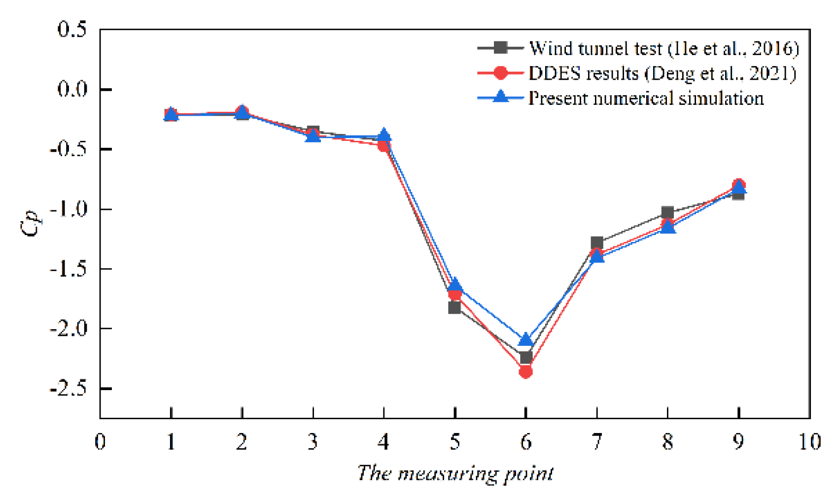
The aerodynamic drag contributes to energy consumption and has a minor impact on train safety. As shown in Figure 4, the main focus of this research was on the changing characteristics of lateral force ($F_y$), lift force ($F_z$), rolling moment ($M_x$), pitching moment ($M_y$), and yawing moment ($M_z$). All the time-varying values were monitored and saved when each time step ends. As shown in Figure 4, the origin of the moment coordinate system of each car was located at the center of gravity of the car, and the local coordinate system was also assigned the same motion as the train.

The pressure distribution on the train surface was also employed to give a comparison of the flow pattern. For a more systematic comparison with existing works, these aerodynamic forces and moments were given as a dimensionless form below:

$$c_s=\frac{F_y}{\frac{1}{2}\rho V^{2}S},$$

(1)

$$c_l=\frac{F_z}{\frac{1}{2}\rho V^{2}S},$$

(2)

$$c_{M_x}=\frac{M_x}{\frac{1}{2}\rho V^{2}SH},$$

(3)

$$c_{M_y}=\frac{M_y}{\frac{1}{2}\rho V^{2}SH},$$

(4)

$$c_{M_z}=\frac{M_z}{\frac{1}{2}\rho V^{2}SH},$$

(5)

$$c_p=\frac{P-P_0}{\frac{1}{2}\rho V^2},$$

(6)

where $F_y$, $F_z$, $M_x$, $M_y$, $M_z$, and $c_p$ are the side force, lift force, rolling moment, pitching moment, yawing moment, and pressure aerodynamic coefficients, respectively; S is the train’s cross-sectional area; $V$ is the resultant velocity in the domain; $P_0$ is the ambient atmospheric pressure; P is the train surface pressure, and H is the height of the train.

3. Validation

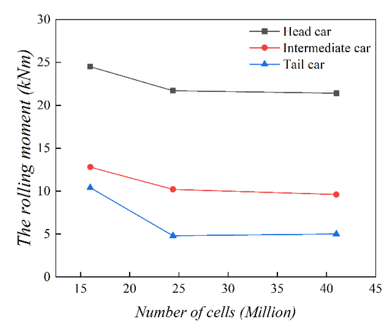
3.1. Grid Sensitivity Test

As an essential reference, the maximum rolling moment of the three cars during the entire passing by the bridge was to compare to test the sensitivity of the grid numbers. Here, the velocity of the train $V_t$ was 300 km/h and that of the crosswind $V_w$ was 20 m/s. The results are presented in Figure 5. It can be seen that the coarse mesh could not produce a convergent result, while the medium and fine meshes provided a good consistency. Accordingly, the coarse mesh was incapable of predicting the flow field around the train, especially near the tail car. In contrast, the medium mesh showed reasonable results and was, therefore, used in the current simulations.

3.2. Experimental Validation

The present methodology was verified using a wind tunnel test conducted at the Central South University. A wind barrier was installed on the bridge, which gave a similar condition as the present simulations. The low-speed test section of the wind tunnel had a length of 18 m, a width of 12 m, and a height of 3.5 m. The wind speed varied between 2 and 20 m/s, and the turbulence rate was less than 2%. The wind pressure is measured using a DTC electronic pressure scanning system. The sampling time for each measurement was 30 s, and the sampling frequency was 330 Hz. As shown in [17], the two-car train model was a 1:25 CRH2 train widely used in China’s high-speed railways. The bridge model used a five-span bridge with 32 m of simply reinforced box girders. Each span was 1280 mm in length. The bridge pier was 400 mm tall, and the gap between the two tracks was 200 mm in the middle. The wind barrier was 0.1 m high, the wind speed was 10 m/s, and the train was stationary, resulting in a 90° yaw angle. The same measuring points were arranged according to [17,20], and the mean pressure coefficient of measuring points 1–9 (can be seen in [17]) on the windward side and the top of the middle carriage are shown in Figure 6.

It can be seen that the numerical simulation results obtained by using the present methodology in this study were generally in good agreement with the previous studies. However, the transition between the windward and the top surfaces of the train (i.e., the measurement points 5 and 6) were found to be slightly smaller than that reported by [17]. The discrepancy of the current results is due to the insufficient prediction accuracy of URANS to solve the flow separation at this region. Nevertheless, the error between the current numerical simulation results and the experimental results is within 10%, sufficient to guide engineering problems.

4. Results

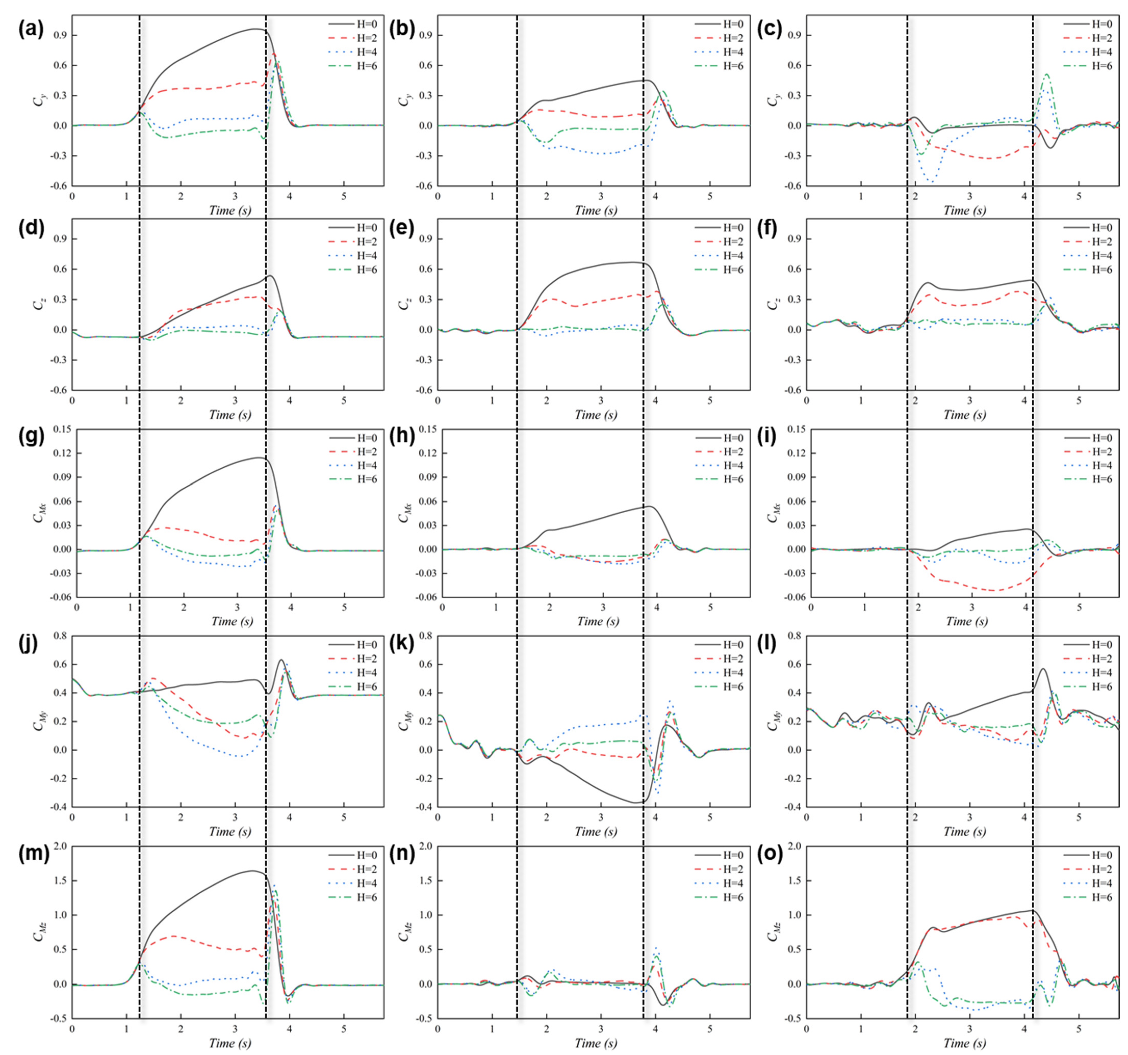
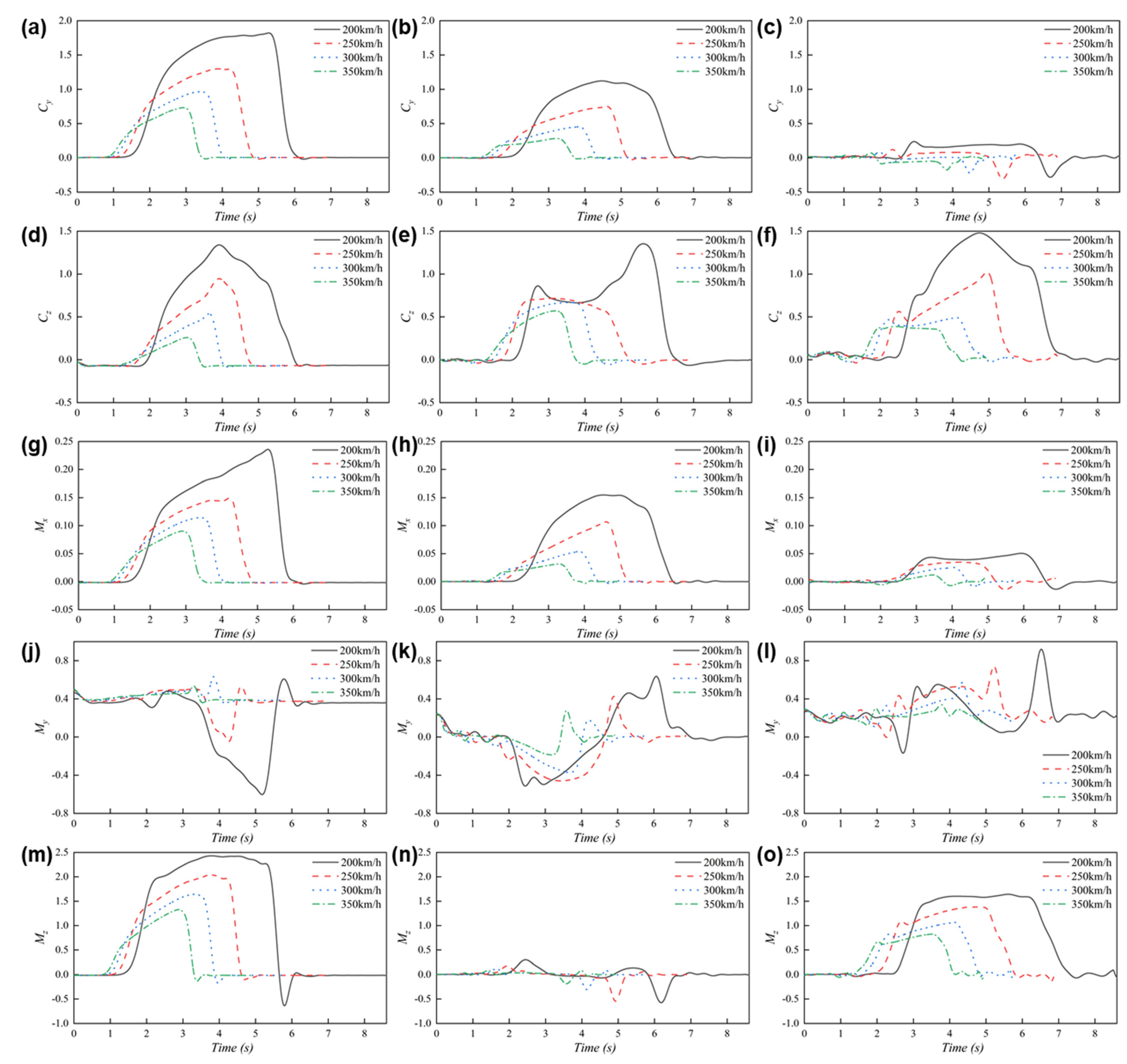
4.1. Time-Varying Aerodynamic Coefficients

Figure 7 shows the time history of the aerodynamic coefficients of each car during the train’s passing from 100 m before the crosswind region to 100 m after the tail car exits. The speed of the train and the crosswind was 83.33 m/s and 20 m/s, respectively. In each figure, the times when the vehicle of interest entered and left the crosswind region were marked to correspond to the change in its aerodynamic coefficients. The results under different wind-protection conditions are included in each figure to compare the protective capacity of the wind barrier and the transient changes of the aerodynamic performance of the train passing through the wind barrier. Each coefficient is given a unified vertical axis range to compare the performance of different cars. The peak-to-peak value of the aerodynamic coefficients obtained when each car of the train entered and left the crosswind area was calculated and shown in

Table 1. Peak-to-peak values of the aerodynamic coefficients when each car entered and left the crosswind region with different wind barriers.

Coefficient	Car	Entering				Exiting
		H = 0 m	H = 2 m	H = 4 m	H = 6 m	H = 0 m	H = 2 m	H = 4 m	H = 6 m
$c_s$	Head	0.441	0.279	0.157	0.228	0.925	0.661	0.544	0.787
	Intermediate	0.219	0.127	0.241	0.204	0.426	0.226	0.460	0.393
	Tail	0.137	0.221	0.552	0.309	0.226	0.169	0.433	0.513
$c_l$	Head	0.092	0.079	0.076	0.033	0.574	0.342	0.244	0.231
	Intermediate	0.370	0.275	0.065	0.009	0.606	0.298	0.313	0.249
	Tail	0.419	0.312	0.074	0.081	0.393	0.227	0.270	0.196
$c_{M_x}$	Head	0.050	0.022	0.017	0.011	0.110	0.049	0.073	0.064
	Intermediate	0.022	0.004	0.005	0.007	0.047	0.021	0.021	0.019
	Tail	0.002	0.030	0.015	0.012	0.032	0.028	0.015	0.010
$c_{M_y}$	Head	0.014	0.097	0.137	0.075	0.238	0.453	0.474	0.462
	Intermediate	0.096	0.078	0.092	0.084	0.532	0.435	0.649	0.481
	Tail	0.223	0.198	0.170	0.124	0.331	0.256	0.392	0.352
$c_{M_z}$	Head	0.772	0.515	0.255	0.283	1.780	1.509	1.668	1.644
	Intermediate	0.116	0.134	0.184	0.215	0.305	0.504	0.830	0.729
	Tail	0.678	0.703	0.158	0.409	0.655	0.490	0.637	0.527

, which numerically assisted the interpretation of fluctuations. Here, the period of “entering” and “exiting” was captured from 0.1 s before the corresponding car started to enter the crosswind region to 0.1 s after it ultimately left it. In this way, the periods for the head, intermediate, and tail car entering the crosswind region were 1.100–1.609 s, 1.409–1.913 s, and 1.713–2.223 s, respectively, and they exited the region at 3.500–4.010 s, 3.810–4.313 s, and 4.113–4.624 s, respectively.

As shown in Figure 7a–c, the lateral force of different cars showed great differences. When there was no wind barrier, the lateral force received from the head car to the tail car decreased in order. The $c_s$ value of the head car in the crosswind area without a wind barrier kept increasing, and the growth rate was the fastest when it just entered this area due to the increase in the blocking area to the crosswind. When it left the crosswind area, the $c_s$ value quickly dropped to 0, which was the same as before entering the region. Wind barrier of different heights gave significant changes to the vehicle’s aerodynamic coefficients: among them, a 2 m-high wind barrier significantly reduced the lateral force of the head car when it passed through the crosswind area, and a 4 m-high wind barrier gave the head car a $c_s$ value of almost 0, while the 6m-high windshield exhibited excessive wind protection, causing the head car to receive a reverse lateral force. Although the wind barriers brought smaller lateral forces, the wind barrier ends essentially changed the local flow pattern, which was reflected in the apparent fluctuations in the aerodynamic coefficients when the train entered and exited the wind barrier, especially for the leaving time. For the intermediate car, the 2 m-high wind barrier showed a good windproof effect, while the higher wall (4 m- and 6 m-high) caused the intermediate car to obtain opposite lateral forces. Due to the existence of the wind barriers, the tail car was subjected to a significant sudden change in lateral force when entering and leaving the crosswind region, and the amplitude was much larger than that without a wind barrier.

As shown in Figure 7d–f, there was no noticeable difference in the maximum lift of the three cars in the crosswind region, but they showed different changes with time: from entering to leaving, the $c_l$ value of the head car increased almost linearly with time, while the growth rate of $c_l$ value acting on the intermediate car gradually slowed, and the tail car reached its maximum value and then remained until it left the crosswind region. The aerodynamic lift was mainly formed by the pressure difference between the upper and lower surfaces of the train. With the presence of wind barriers, the flow rate under the train was more directly suppressed, the lift of the train was, therefore, effectively weakened. Among them, the 4 m- and 6 m-high wind barriers almost completely eliminated the lift received by the train because the airflow both above and below the car body was synchronously filtered, but they gave a relatively high $c_l$ value when the train left the crosswind region.

As a combination of lateral and lift forces, the overturning moment acting on different cars passing through the crosswind region without a wind barrier showed a similar trend with different values, as exhibited in Figure 7g–h. The wind barriers always restrained the $c_{M_x}$ value of the train to a large extent. It should be noted that the wind barrier with a 2 m height can cause the tail car to produce a reverse overturning moment, which was even more significant than the positive $c_{M_x}$ value received without any wind barriers. It can be attributed to the effect of the side force shown in Figure 7c.

A significant difference was found in the trend and the value of the pitching moments of different cars. The pitching moments of the head and tail cars were always positive, while the intermediate car showed a negative $c_{M_y}$ value for more than half of the time. The wind barriers try to make the $c_{M_y}$ value of each car closer to 0, but their effect was not monotonously increasing with the height of the barrier.

A low yawing moment was found when the intermediate car passed through the crosswind region, and those of the head and the tail cars changed significantly because they were only connected to other vehicles at one end. The 2 m-high wind barriers effectively reduced the $c_{M_z}$ value acting on the head car and had almost no effect on the tail car. A higher wind barrier reduced them to 0 and even a negative value. When leaving the crosswind area, the fluctuations that the end of the wind barrier brought to the head car were the most obvious among all aerodynamic coefficients because the difference in lateral force between the front and rear of a car was the largest. It should be noted that the reason why the intermediate car was obviously different from the head and the tail cars for $c_{M_y}$ and $c_{M_z}$ values is that it was geometrically symmetrical in the length direction, while the head and tail cars have a strong asymmetric flow due to the presence of streamlined structures so that different time-varying $c_{M_y}$ and $c_{M_z}$ values were generated.

Figure 7 and Table 1 show that almost all the aerodynamic coefficient fluctuations of cars exiting the crosswind region were larger than that entering the region. Their changes also reflected the effect of the height of the wind barrier on the wind-protection performance, taking into consideration the over-protection.

The influence of the running speed of the train on the aerodynamic forces and moments is also shown in Figure 8. The table showing their peak-to-peak value of the aerodynamic coefficients when each car of the train entering and leaving the crosswind area is also given in

Table 2. Peak-to-peak values of the aerodynamic coefficients when each car entered and left the crosswind region with different running speeds.

Coefficient	Car	Entering				Exiting
		200 km/h	250 km/h	300 km/h	350 km/h	200 km/h	250 km/h	300 km/h	350 km/h
$c_s$	Head	0.993	0.653	0.441	0.312	1.744	1.222	0.925	0.723
	Intermediate	0.604	0.314	0.219	0.097	0.852	0.693	0.426	0.279
	Tail	0.206	0.126	0.137	0.099	0.417	0.329	0.226	0.122
$c_l$	Head	0.603	0.227	0.092	0.041	0.830	0.882	0.574	0.324
	Intermediate	0.790	0.633	0.370	0.092	1.253	0.484	0.606	0.533
	Tail	0.649	0.500	0.419	0.325	0.951	0.914	0.393	0.253
$c_{M_x}$	Head	0.111	0.075	0.050	0.034	0.233	0.142	0.110	0.086
	Intermediate	0.069	0.032	0.022	0.005	0.117	0.094	0.047	0.029
	Tail	0.038	0.013	0.002	0.004	0.055	0.037	0.032	0.019
$c_{M_y}$	Head	0.098	0.019	0.014	0.019	1.112	0.579	0.238	0.132
	Intermediate	0.347	0.193	0.096	0.062	0.508	0.520	0.532	0.460
	Tail	0.699	0.438	0.223	0.156	0.717	0.485	0.331	0.111
$c_{M_z}$	Head	1.555	1.117	0.772	0.562	2.902	2.063	1.780	1.425
	Intermediate	0.167	0.119	0.116	0.060	0.597	0.485	0.305	0.199
	Tail	1.267	0.993	0.678	0.517	1.029	0.837	0.655	0.499

.

Compared to the influence given by the height of the wind barrier, the running speed of the train seemed to provide a difference in the aerodynamic coefficient values instead of the developing pattern. With the same crosswind, when the train runs at a lower speed, a larger yaw angle can result from a synthesis between the train speed and the crosswind. Therefore, at a lower vehicle speed, it was easier to obtain a greater aerodynamic coefficient when calculating the aerodynamic coefficient. On the one hand, the yaw angle directly changed the contribution of the resultant wind to the lateral force of the train. On the other hand, it also changed the flow pattern near the train body, which may cause a mode change in the time-varying force coefficients of the train, as shown in Figure 8b,e. According to Table 2, for the aerodynamic coefficients’ peak-to-peak value when each car of the train entered and left the crosswind region, the value-based sorting relationship among the head, the intermediate, and the tail cars was almost the same regardless of the running speed of the train. For $c_s$, $c_z$ and $c_{M_x}$, the value of the head car to the tail car was decremented, and the opposite relationship could be found in $c_{M_y}$. For $c_{M_z}$, the head car always had the highest value, while the intermediate car had the lowest value. Moreover, as the train speed increased, the obtained value of various aerodynamic coefficients always showed a decreasing trend.

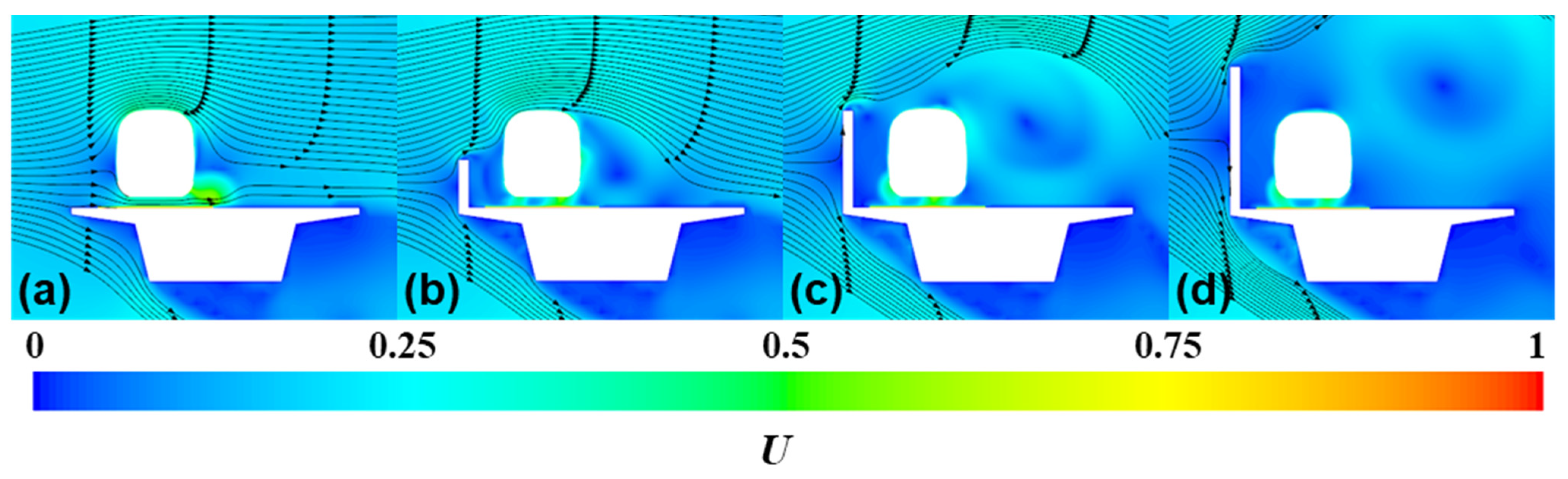
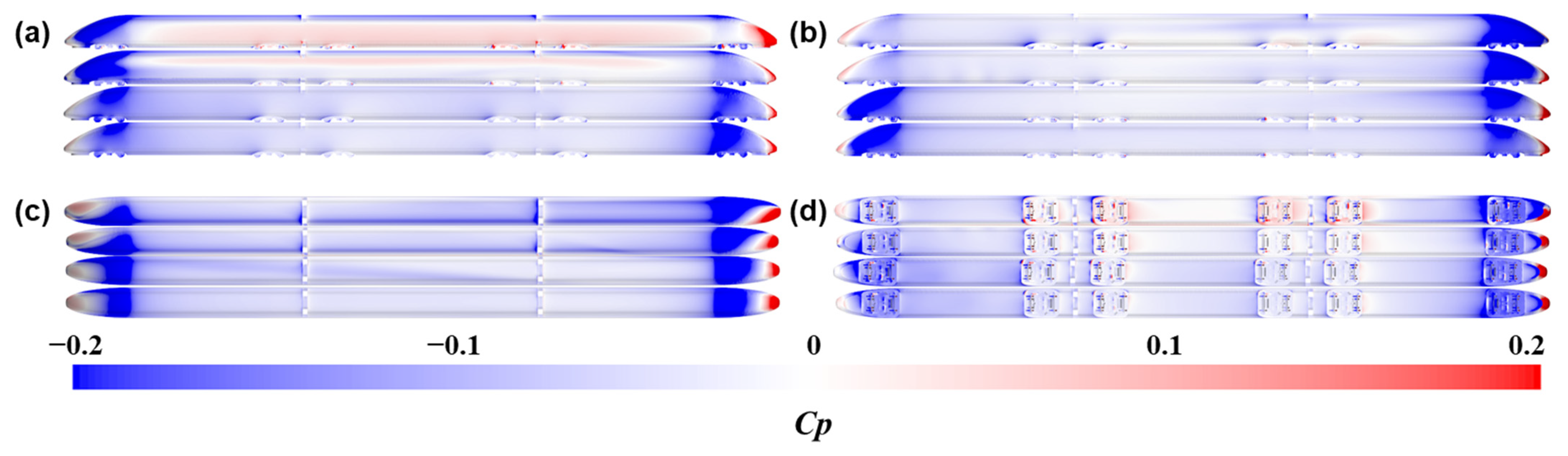
4.2. Flow Field and Train Surface Pressure

Figure 9 shows the distribution of the dimensionless velocity U and the streamlines projected on the y-z plane at the middle length of the head car downstream various wind barriers. Here, the value of U can be calculated as:

$$U=\frac{u}{V},$$

(7)

where u is the velocity of the flow in the domain obtained by the numerical result. This comparison was based on the time when the train arrived in the middle of the crosswind region. As the height of the wind barrier increased, its blocking effect on the crosswind became greater, and the airflow acted less directly on the train but moved up and down under the guidance of the wall. When there was no wind barrier, the speed distribution around the vehicle was almost symmetrical with a slight yaw angle, and the existence of the windshield broke this symmetry. As the height of the wind barrier increased, the higher speed region at the bottom of the train body gradually moved from the leeward side to the upwind side of the train. Under the protection of the 2 m high wind barrier, a low-speed region caused by the vortex was formed near half the height of the leeward side of the train. The height and scale of this vortex also increased with the height of the wind barrier, as shown in Figure 9b,d. There was also a lower speed in the area between the windshield and the car body. The high-speed area on the top of the train body only existed in the working condition where the wind barrier was less than 2 m.

Figure 10 shows the pressure distribution on the surfaces of the train when it was located in the same position as Figure 9 from four different perspectives. The pressure distribution on the windward side of the train is shown in Figure 10a. When the train was running without the protection of a wind barrier, the windward side of the nose of the head car obtained the largest positive pressure area, and wind barriers in different heights significantly reduced the area, and there was little difference among these cases with wind barriers. When the heights of the wind barriers wall were 0 m and 2 m, the streamlined structure of the tail car was almost entirely covered by negative pressure, while the 4 m and 6 m barriers weakened the negative pressure near the nose. In addition to the streamlined structure of the head and tail cars, the absence of the wind barrier led to the largest positive pressure area distributed in the middle and lower areas of the main body of the train, and the 2 m high wind barrier made the area of this region smaller and upward. This area of positive pressure disappeared when a higher wind barrier existed. This was consistent with the results caused by the flow pattern shown in Figure 9. For the leeward side shown in Figure 10b, as the height of the wind barrier increased, the negative pressure value and area distributed on the head car were reduced, while the negative pressure on the tail car was strengthened. There was no significant difference in the pressure distribution on the leeward side of the main train body. It can be seen from Figure 10c that the spanwise symmetry of the positive pressure distribution in the nose area of the head car increased with the height of the wind barrier, and the negative pressure distribution at the tail car was also the same. The pressure on the top surface of the train under the protection of the high wind barriers was closer to zero. Low negative pressure was distributed under the train, and as the wind barrier height increased, the positive pressure in the bogie cabins was weakened.

4.3. Dynamic Response

The transient aerodynamic load during the passing was inputted into the train–bridge coupled dynamic system to realize a dynamic analysis of running safety. The train–bridge system can be divided into train and track–bridge subsystems. For the sake of simplicity, the current study did not describe the dynamic system model specifically, which can be seen in Deng’s research [17].

According to the previous studies, the head car was exposed to higher operational safety risks than the intermediate and tail cars due to more significant aerodynamic fluctuations. The running safety of the head car was, therefore, focused on studying the effect of the wind barrier and running speed on the train DC and WLRR. The posture changes of the train passing through the crosswind region under different wind barrier conditions and at different speeds were also studied.

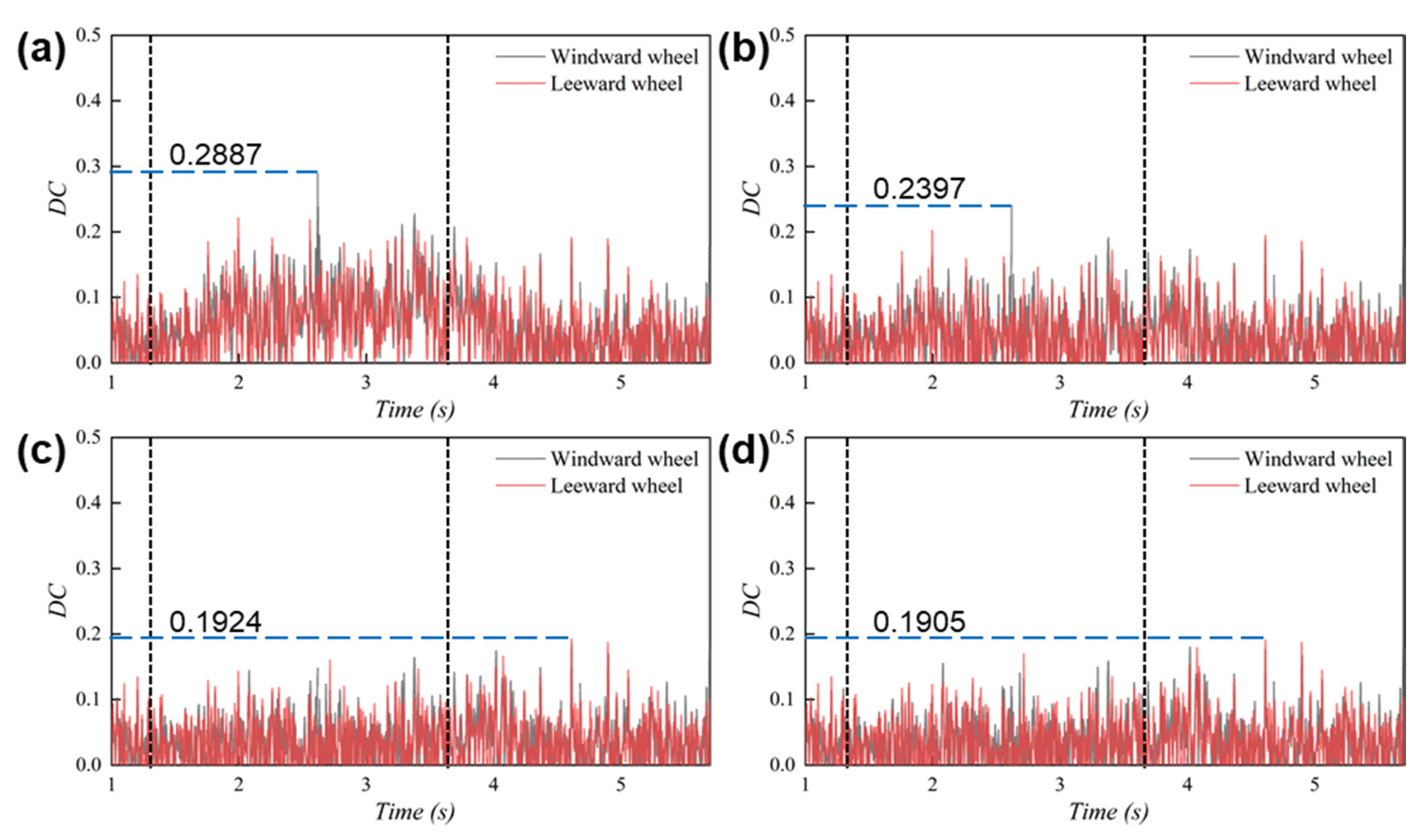
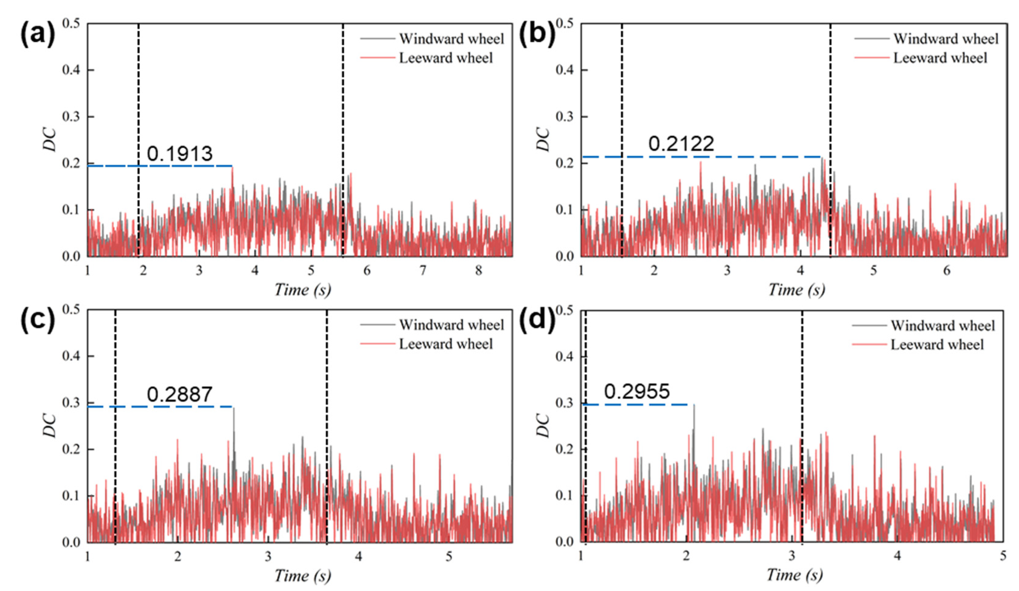
4.3.1. Derailment Coefficient

The train derailment coefficient of the trains can be calculated by the contact force of the wheels according to the TB10621-2009 standard, which can be given:

$$DC=\frac{Q}{P}\le 0.8,$$

(8)

where Q and P are the lateral and vertical forces acting on the wheels, respectively. Figure 11 and Figure 12 give the time-varying DC values of the first wheelset of the head car under different wind-protection conditions and running speeds, and the two black dotted lines in each figure means the time points when the wheel entered and left the crosswind region, respectively.

When the train passed the bridge without a wind barrier, the DC of the first wheelset showed higher values when the train ran in the crosswind region. No obvious difference was found in the DC performance of the windward and leeward wheels. The windward wheel gave the maximum DC value found in the whole running for the 0 m and 2 m wind barrier, while the leeward wheel exhibited a higher maximum value when the wind barrier was higher. The maximum DC value kept decreasing from 0.2887 to 0.1905 with the increase in the height of wind barriers, although the difference between 4 m and 6 m height was not apparent. As shown in Figure 12, the time-axis was not on the same scale due to the different speeds of the train. It can be seen that as the running speed of the train increased, the fluctuation range and maximum of the DC value of the first wheel were both increased. The maximum value of the DC always occurred when the train passes the crosswind region, and the higher maximum of the DC value was presented when the train ran with higher speeds.

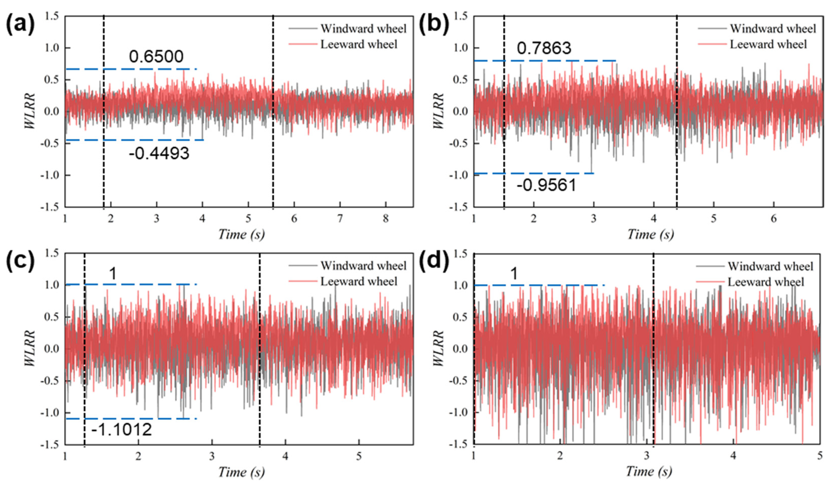
4.3.2. Wheel Load Reduction Rate

When the train ran at high speed, the wheels moved up and down with the vibration process, and the wheel weight of the wheelset increased or decreased. Even if the lateral force on the side of the reduced wheel weight is small (or even no), there may be lateral relative displacement with the wheels, which leads to a derailment. The criteria of WLRR was, therefore, considered in the evaluation of the running safety:

$$\{\begin{array}{c}\frac{\Delta P}{P}\le 0.8\\ \frac{\Delta P}{P}>0.8, \Delta t<0.035s\end{array}$$

(9)

where ΔP is the load reduction in the wheel load, P is the average static wheel load of the wheelset, and $\Delta t$ is the maximum overrun duration. Figure 13 and Figure 14 give the time-varying WLRR values of the first wheelset of the head car under different wind-protection conditions and running speeds.

No noticeable difference in the WLRR value was found when the train ran on a bridge with a wind barrier at different heights. In addition, both the fluctuation amplitude and maximum of the WLRR value increased with the running speed.

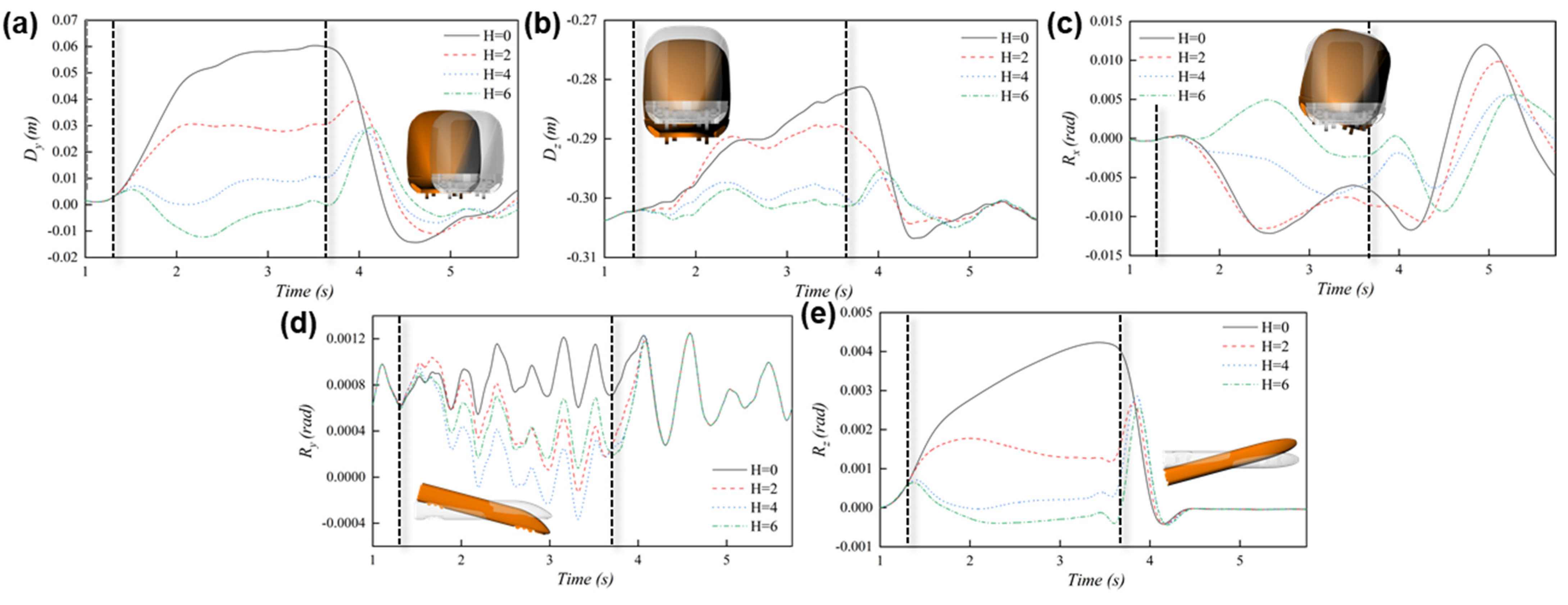
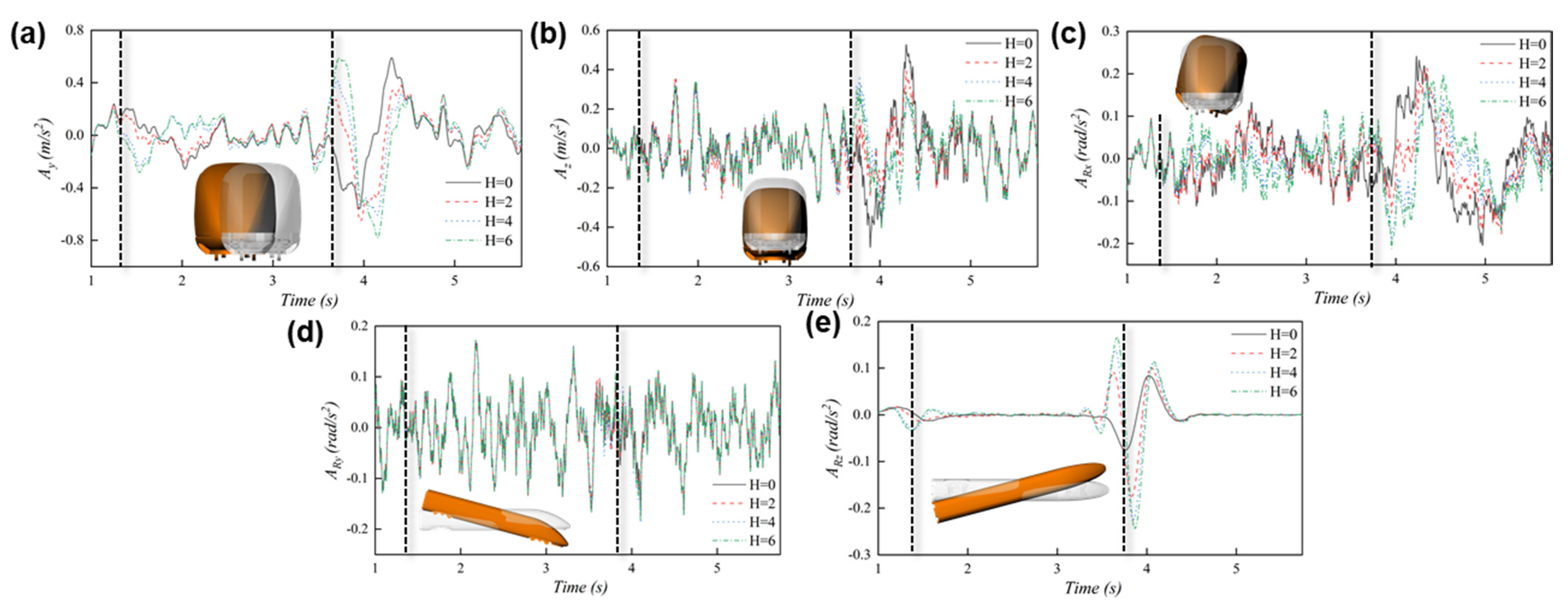
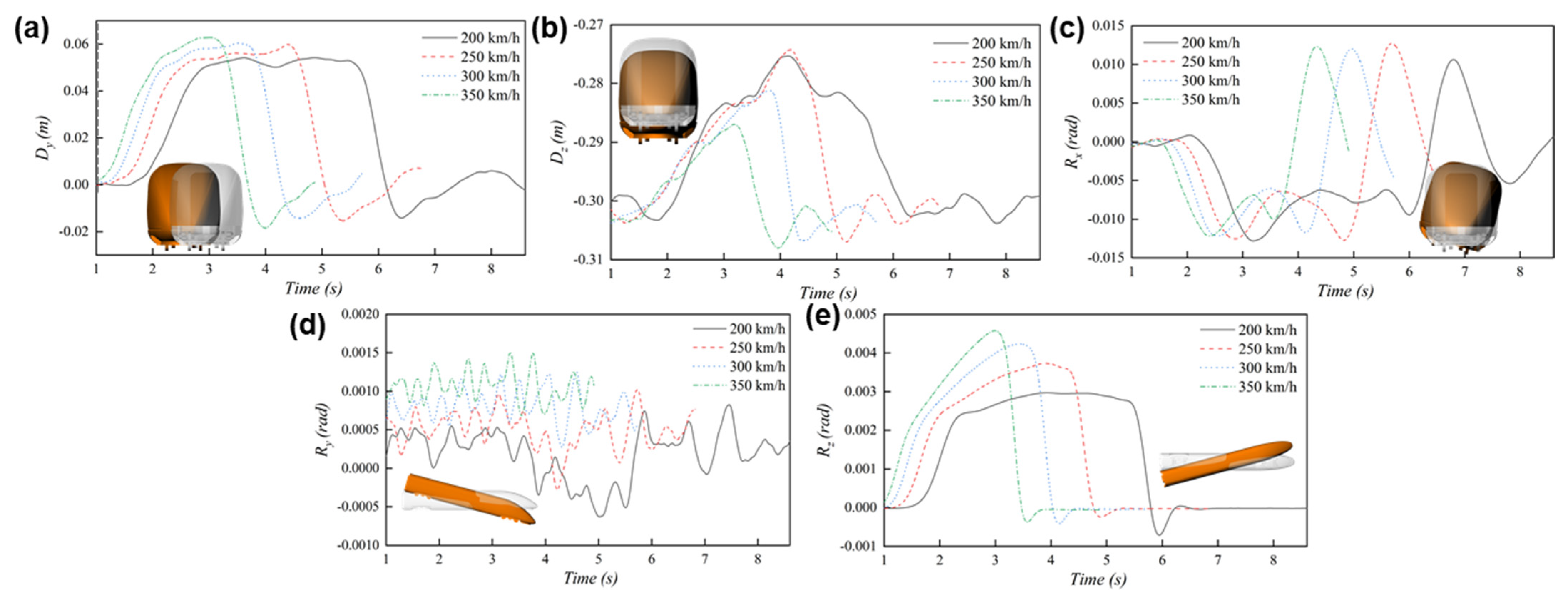
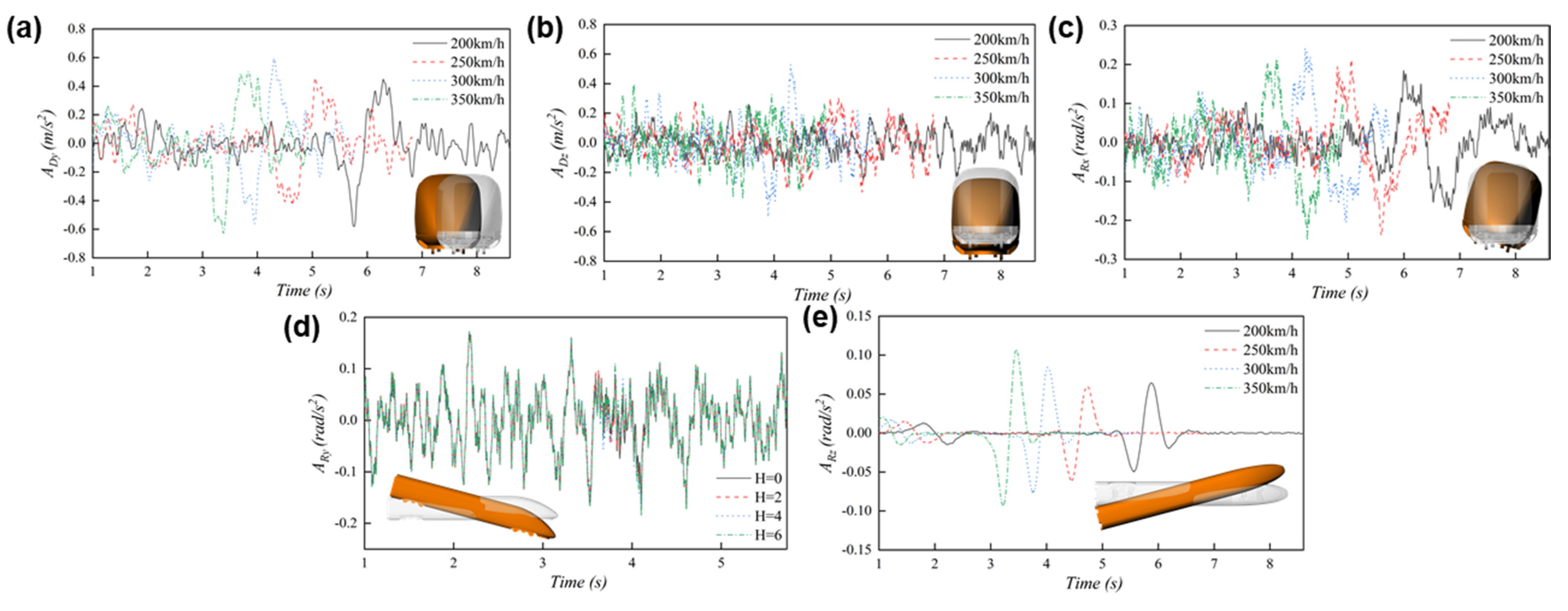
4.3.3. Running Posture

Furthermore, the DC and WLRR and based on the coordinate system given in Figure 4, the train–bridge coupled dynamic system provides the posture with respect to changes in the train passing through the crosswind area under different wind barrier conditions and at different speeds. As in Section 4.3.1 and Section 4.3.2, the changes and acceleration of the head car in five degrees of freedom (lateral and vertical displacement and rotation in three directions) were compared and analyzed.

Figure 15 shows the changes of different degrees of freedom indexes when the train passed the bridge under the protection of different heights of the windshield. In the figure, Dy, Dz, Rx, Ry, Rz are the lateral and vertical displacements (unit: m) of the head car and the rotation of the x, y, and z axes (unit: rad). Figure 16 shows their acceleration, where Ay, Az, A_Rx, A_Ry, A_Rz are the accelerations of Dy, Dz, Rx, Ry, Rz, respectively. The diagram of the running posture of the train is also given in each figure, where the transparent one means the original position, and another is the posture caused by the crosswind. As shown in Figure 15a, when the train entered the crosswind region, a displacement corresponding to the crosswind was applied to the train, among them, the 0 m and 2 m height barriers could not effectively reduce this displacement, while the 4 m height barrier always kept the head car move laterally with 0.01 m, which was regarded as the best wind-protection effect. However, a displacement opposite to the crosswind direction was found at the train under a 6 m height wind barrier due to the over-protection. The crosswind raised the height position of the head car while the barriers weakened this effect, where the 4 m height and 6 m height gave a similar response, as shown in Figure 15b. The crosswind tended to provide a negative Rx value to make the train overturn, where the 2 m height wind barrier seemed not to bring any protection. Same as the performance of the Dy, the 4 m height barrier effectively decreased the Rx while the higher one gave an over-protection. Many fluctuations were found in the change in Ry; the presence of the wind barriers always provided a good reduction in the Ry value to ease the pitching moment of the head car. As shown in Figure 15d, the varying yawing moment showed a sensitive change to the height of the wind barrier. As shown in Figure 16, the difference among the accelerations along five degrees of freedom of the head car was not as evident as the displacements and rotations. Although the wind barrier can effectively maintain the running posture of the train in the crosswind region, its existence will bring greater fluctuations when the train enters or leaves the barrier region.

Similarly, Figure 17 shows the changes of different degrees of freedom indexes when the train passed the bridge at different speeds, and Figure 18 gives their accelerations. In addition to the time difference brought about by different speeds, the sensitivity of Dy and Rx to the running speed of the train was slight, as shown in Figure 17a,c. A higher running speed resulted in smaller Dz and greater Ry and Rz. The acceleration also exhibited complex changes over time, but the peak value of acceleration always increased with increasing speed.

5. Conclusions

The URANS model was used to obtain the transient aerodynamic load of the train passing a bridge with a crosswind region. Based on the variance characteristics of the train derailment coefficient and wheel load reduction rate, the effect of wind barrier height and the running speed on running safety were also studied. The time-varying changes of the train’s running posture and acceleration in five degrees of freedom were also compared and analyzed. The main conclusions can be concluded as below:

• Wind barriers of different heights provided significant changes to the train’s aerodynamic coefficients. The ends of the wind barrier essentially changed the local flow pattern, which is reflected in the obvious fluctuations in the aerodynamic coefficients when the train enters and exits the wind barrier, especially for the leaving. The running speed of the train gives a difference in the aerodynamic coefficient values instead of the developing pattern.
• The maximum Derailment coefficient continued to decrease with the increase in the height of wind barriers, which hardly affected the wheel load reduction rate. The fluctuation range and maximum value of the Derailment coefficient and the wheel load reduction rate of the first wheel increased with the train speed.
• For a general high-speed train running on a bridge in the crosswind, the 4 m high wind barrier was proven to effectively protect the running posture of the train, while the 6 m high one consistently exhibited over-protection. The 2 m high wind barrier had no apparent influence on the train’s posture.
• Further work may lie in the optimization of the severe aerodynamic changes and safety threats of the train passing by the wind barrier ends. It may be achieved by adding a longitudinally extended transition wall at the ends.

References

1. Guo, Z.; Liu, T.; Chen, Z.; Xia, Y.; Li, W.; Li, L. Aerodynamic influences of bogie’s geometric complexity on high-speed trains under crosswind. J. Wind. Eng. Ind. Aerodyn. 2020, 196, 104053. [Google Scholar] [CrossRef]
2. Deng, E.; Yang, W.; He, X.; Ye, Y.; Zhu, Z.; Wang, A. Transient aerodynamic performance of high-speed trains when passing through an infrastructure consisting of tunnel–bridge–tunnel under crosswind. Tunn. Undergr. Space Technol. 2020, 102, 103440. [Google Scholar] [CrossRef]
3. Guo, Z.; Liu, T.; Chen, Z.; Liu, Z.; Monzer, A.; Sheridan, J. Study of the flow around railway embankment of different heights with and without trains. J. Wind. Eng. Ind. Aerodyn. 2020, 202, 104203. [Google Scholar] [CrossRef]
4. Gallagher, M.; Morden, J.; Baker, C.; Soper, D.; Quinn, A.; Hemida, H.; Sterling, M. Trains in crosswinds—Comparison of full-scale on-train measurements, physical model tests and CFD calculations. J. Wind. Eng. Ind. Aerodyn. 2018, 175, 428–444. [Google Scholar] [CrossRef] [Green Version]
5. Yang, W.; Deng, E.; Zhu, Z.; He, X.; Wang, Y. Deterioration of dynamic response during high-speed train travelling in tunnel–bridge–tunnel scenario under crosswinds. Tunn. Undergr. Space Technol. 2020, 106, 103627. [Google Scholar] [CrossRef]
6. Diedrichs, B.; Sima, M.; Orellano, A.; Tengstrand, H. Crosswind stability of a high-speed train on a high embankment. Proc. Inst. Mech. Eng. Part F J. Rail Rapid Transit 2007, 221, 205–225. [Google Scholar] [CrossRef]
7. Noguchi, Y.; Suzuki, M.; Baker, C.; Nakade, K. Numerical and experimental study on the aerodynamic force coefficients of railway vehicles on an embankment in crosswind. J. Wind. Eng. Ind. Aerodyn. 2019, 184, 90–105. [Google Scholar] [CrossRef]
8. Barcala, A.M.; Meseguer, J. An experimental study of the influence of parapets on the aerodynamic loads under cross wind on a two-dimensional model of a railway vehicle on a bridge. Proc. Inst. Mech. Eng. Part F J. Rail Rapid Transit 2007, 221, 487–494. [Google Scholar] [CrossRef]
9. Xia, H.; Guo, W.; Zhang, N.; Sun, G. Dynamic analysis of a train–bridge system under wind action. Comput. Struct. 2008, 86, 1845–1855. [Google Scholar] [CrossRef]
10. Song, M.-K.; Noh, H.-C.; Choi, C.-K. A new three-dimensional finite element analysis model of high-speed train–bridge interactions. Eng. Struct. 2003, 25, 1611–1626. [Google Scholar] [CrossRef]
11. Kozmar, H.; Procino, L.; Borsani, A.; Bartoli, G. Sheltering efficiency of wind barriers on bridges. J. Wind. Eng. Ind. Aerodyn. 2012, 107–108, 274–284. [Google Scholar] [CrossRef] [Green Version]
12. Bitog, J.; Lee, I.-B.; Shin, M.-H.; Hong, S.-W.; Hwang, H.-S.; Seo, I.-H.; Yoo, J.-I.; Kwon, K.-S.; Kim, Y.-H.; Han, J.-W. Numerical simulation of an array of fences in Saemangeum reclaimed land. Atmospheric Environ. 2009, 43, 4612–4621. [Google Scholar] [CrossRef]
13. Hong, S.-W.; Lee, I.-B.; Seo, I.-H. Modelling and predicting wind velocity patterns for windbreak fence design. J. Wind. Eng. Ind. Aerodyn. 2015, 142, 53–64. [Google Scholar] [CrossRef]
14. Chen, N.; Li, Y.; Wang, B.; Su, Y.; Xiang, H. Effects of wind barrier on the safety of vehicles driven on bridges. J. Wind. Eng. Ind. Aerodyn. 2015, 143, 113–127. [Google Scholar] [CrossRef]
15. Xue, F.; Han, Y.; Zou, Y.; He, X.; Chen, S. Effects of wind-barrier parameters on dynamic responses of wind-road vehicle–bridge system. J. Wind. Eng. Ind. Aerodyn. 2020, 206, 104367. [Google Scholar] [CrossRef]
16. Gu, H.; Liu, T.; Jiang, Z.; Guo, Z. Research on the wind-sheltering performance of different forms of corrugated wind barriers on railway bridges. J. Wind. Eng. Ind. Aerodyn. 2020, 201, 104166. [Google Scholar] [CrossRef]
17. Deng, E.; Yang, W.; He, X.; Zhu, Z.; Wang, H.; Wang, Y.; Wang, A.; Zhou, L. Aerodynamic response of high-speed trains under crosswind in a bridge-tunnel section with or without a wind barrier. J. Wind. Eng. Ind. Aerodyn. 2021, 210, 104502. [Google Scholar] [CrossRef]
18. Deng, E.; Yang, W.; Lei, M.; Zhu, Z.; Zhang, P. Aerodynamic loads and traffic safety of high-speed trains when passing through two windproof facilities under crosswind: A comparative study. Eng. Struct. 2019, 188, 320–339. [Google Scholar] [CrossRef]
19. Chu, C.-R.; Chang, C.-Y.; Huang, C.-J.; Wu, T.-R.; Wang, C.-Y.; Liu, M.-Y. Windbreak protection for road vehicles against crosswind. J. Wind. Eng. Ind. Aerodyn. 2013, 116, 61–69. [Google Scholar] [CrossRef]
20. He, X.; Zou, Y.; Wang, H.; Han, Y.; Shi, K. Aerodynamic characteristics of a trailing rail vehicles on viaduct based on still wind tunnel experiments. J. Wind. Eng. Ind. Aerodyn. 2014, 135, 22–33. [Google Scholar] [CrossRef]
Figure 1. Geometric models employed in the numerical simulation: (a) The train model; (b) A realistic CRH3 train; (c) The bridge model and location of the train; (d) The length components of the train.
Applsci 11 04126 g001
Figure 2. Computational domain and boundary conditions: (a) An overall side view; (b) The side view of the overset region; (c) The front view of the computational domain; (d) The front view of the overset region.
Applsci 11 04126 g002
Figure 3. Computational mesh employed in the simulations: (a) front view of mesh density in the computational domain; (b) side view of mesh density in the computational domain; (c) mesh distribution on the surface of the nose; (d) the prism layer cells attaching to the train surface.
Applsci 11 04126 g003
Figure 4. The Parameter definition and the origin of the moment coordinate system.
Applsci 11 04126 g004
Figure 5. Maximum rolling moment of three cars predicted by different meshes (in V t = 300 km/h; V w = 20 m/s).
Applsci 11 04126 g005
Figure 6. The distribution of the pressure on the train surface obtained by the present and previous studies.
Applsci 11 04126 g006
Figure 7. The time-varying aerodynamic coefficients of each car of the train passing the bridge with various wind barriers: (a) c s of the head car; (b) c s of the intermediate car; (c) c s of the tail car; (d) c l of the head car; (e) c l of the intermediate car; (f) c l of the tail car; (g) c M x of the head car; (h) c M x of the intermediate car; (i) c M x of the tail car; (j) c M y of the head car; (k) c M y of the intermediate car; (l) c M y of the tail car; (m) c M z of the head car; (n) c M z of the intermediate car; (o) c M z of the tail car.
Applsci 11 04126 g007
Figure 8. The time-varying aerodynamic coefficients of each car of the train passing the bridge with various running speeds: (a) c s of the head car; (b) c s of the intermediate car; (c) c s of the tail car; (d) c l of the head car; (e) c l of the intermediate car; (f) c l of the tail car; (g) c M x of the head car; (h) c M x of the intermediate car; (i) c M x of the tail car; (j) c M y of the head car; (k) c M y of the intermediate car; (l) c M y of the tail car; (m) c M z of the head car; (n) c M z of the intermediate car; (o) c M z of the tail car.
Applsci 11 04126 g008
Figure 9. Distribution of U and the streamlines projected on the y-z plane at the middle length of the head car with various wind barriers: (a) H = 0 m; (b) H = 2 m; (c) H = 4 m; (d) H = 4 m.
Applsci 11 04126 g009
Figure 10. Distribution of c p on the surface of the train with various wind barriers: (a) Windward side; (b) Leeward side; (c) Roof; (d) Bottom. The heights of the wind barrier are 0 m to 6 m from top to bottom in each figure.
Applsci 11 04126 g010
Figure 11. Time-varying DC values of the first wheelset of the head car under various wind-protection conditions: (a) H = 0 m; (b) H = 2 m; (c) H = 4 m; (d) H = 6 m.
Applsci 11 04126 g011
Figure 12. Time-varying DC values of the first wheelset of the head car with various running speeds: (a) 200 km/h; (b) 250 km/h; (c) 300 km/h; (d) 350 km/h.
Applsci 11 04126 g012
Figure 13. Time-varying WLRR values of the first wheelset of the head car with various wind-protection conditions: (a) H = 0 m; (b) H = 2 m; (c) H = 4 m; (d) H = 6 m.
Applsci 11 04126 g013
Figure 14. Time-varying WLRR values of the first wheelset of the head car with various running speeds: (a) 200 km/h; (b) 250 km/h; (c) 300 km/h; (d) 350 km/h.
Applsci 11 04126 g014
Figure 15. Time-varying values of the indicators along five degrees of freedom of the head car with various wind barriers: (a) Dy; (b) Dz; (c) Rx; (d) Ry; (e) Rz.
Applsci 11 04126 g015
Figure 16. Time-varying values of the accelerations along five degrees of freedom of the head car with various wind barriers: (a) Ay; (b) Az; (c) ARx; (d) ARy; (e) ARz.
Applsci 11 04126 g016
Figure 17. Time-varying values of the indicators along five degrees of freedom of the head car with various running speeds: (a) Dy; (b) Dz; (c) Rx; (d) Ry; (e) Rz.
Applsci 11 04126 g017
Figure 18. Time-varying values of the accelerations along five degrees of freedom of the head car with various running speeds: (a) Ay; (b) Az; (c) ARx; (d) ARy; (e) ARz.
Applsci 11 04126 g018