Visual Simulation of Turbulent Foams by Incorporating the Angular Momentum of Foam Particles into the Projective Framework

Abstract

In this paper, we propose an angular momentum-based advection technique that can express the turbulent foam effect. The motion of foam particles, which are strongly bound to the motion of the underlying fluid, is viscous, and sometimes clumping problems occur. This problem is a decisive factor that makes it difficult to express realistic foam effects. Since foam particles, which are secondary effects, depend on the motion of the underlying water, in order to exaggerate the foam effects or express more lively foam effects, it is inevitable to tune the motion of the underlying water and then readjust the foam particles. Because of such a cumbersome process, the readjustment of the foam effects requires a change in the motion of the underlying water, and it is not easy to produce such a scene because the water and foam effects must change at the same time. In this paper, we present a method to maintain angular momentum-based force from water particles without tuning the motion of the underlying water. We can restore the lost turbulent flow by additional advection of foam particles based on this force. In addition, our method can be integrated with screen-space projection frameworks, allowing us to fully embrace all the advantages of this approach. In this paper, the turbulence of the foam particles was improved by minimizing the viscous motion of the foam particles without tuning the motion of the underlying water, and as a result, lively foam effects can be expressed.

1. Introduction

In fluid simulations dealing with water, smoke, fire, etc., studies have been continuously attempted to express turbulent flow by restoring details lost by numerical dissipation: Particle-based fluids techniques such as MPM (Material Point Method) [1,2], FLIP (Fluid-Implict Particle) [3,4,5], APIC (Affine Particle-In-Cell) [6,7], Polynomial PIC [8], and SPH (Smoothed Particle Hydrodynamics) [9,10,11] are useful in creating splashes and expressing free surfaces in detail, so they have been widely used in computer graphics in recent years. Chen et al. proposed a particle-grid hybrid framework for synthesizing turbulent flow [12]. Zhao et al. proposed a technique to express fluid turbulence more efficiently by upsampling the grid structure [13]. Yoon et al. proposed a technique to express turbulent smoke by upsampling the vortex particles method to a higher resolution grid [14]. Weissmann et al. expressed vorticity using vortex filaments [15]. Barnat and Pollard expressed more accurate vortex filaments by improving the resampling scheme proposed in the above technique [16].

Physically-based fluid simulations often deal with turbulent flows expressed in fluid–solid interactions or large fluid bodies. Key issues in expressing turbulent fluids are the generation and preservation of small-scale details: Methods have been proposed to solve this problem based on physics [17,18,19,20,21] or noise and texture [22,23,24]. Depending on the fluid materials corresponding to these issues, the expression technique should be modeled differently. For example, when expressing water, the motion of the main body and the turbulent flow are important, but the secondary effects (e.g., splash, foam, bubble, mist, etc.) resulting from it are also important. However, most approaches have a strong linking structure in which secondary effects are expressed only by the underlying water simulation. Since it is difficult to independently control the motion of the foam effects created in the strong linking structure, even the motion of the underlying water needs to be modified in order to control the motion of the foam particles in detail. The Navier–Stokes equation is often used to simulate the splash or foam effects with complicated motion in wild water flows. However, in the process of calculating the foam particles, it is necessary to check all the water particles, so a huge computational cost and resources are required [25]. In addition, since it is bound to the movement of water particles, it is difficult to properly express intrinsic patterns or styles expressed in foam. Recently, Kim et al. expressed foam effects efficiently using 2D projective space and expressed intrinsic patterns of foam by proposing a clamping function based on curvature [26,27]. This method tried to express intrinsic patterns by controlling foam generation like a curvature-based mask map. However, since it does not affect the motion, it does not dynamically enhance the motion of the foam particles.

In the existing methods, it is difficult to express wave patterns or dynamic motion of foam because the foam particles are advected while being strongly bound to the underlying water simulation. In addition, it is difficult to intuitively control the foam effects because the user has to modify the underlying water to control the secondary effects. In this paper, not only foam particles are expressed based on the motion of the underlying water, but also lively foam effects can be expressed by adding the angular momentum of water particles to the foam advection process.

Problem Statement

Before entering into the details of the problem statement, the following summarizes the shortcomings of the prior technique for realistically simulating foam patterns:

• Foam patterns are generated only by the depth-based curvature difference, not by water flow.
• While this does not appear to be a mask map, it is difficult to depict detailed foam motion for reasons (1).
• It’s particularly challenging to convey the complexity of foam, which is largely dependent on water velocity, such as the movement of a bubble being drawn in.

In general, secondary effects such as foam are based on the motion of water particles. Among the various secondary effects, foam particles not only have intrinsic patterns, but also exhibit dynamic and complex movements compared to water particles. Since it is strongly linked to the underlying water simulation, if there is little movement of the water particles, the foam particles are clumped. However, if the turbulence of water particles is strongly applied to express the foam effect, the water flow itself is severely deformed. Kim et al. proposed a curvature-based clamping function to alleviate the clumping problem of foam [26,27] (see Figure 1).

As shown in Figure 1, intrinsic patterns of foam can be expressed using depth-based curvature flow, but like a mask map, it only affects the foam generation process, so the movement of foam particles still depends only on the underlying water. Recently, Kim and Lee proposed a technique of advection according to the type of foam by dividing it into wave and surface [26]. They expressed a cloud-like surface foam by adding a spring force such as SPH, but still rely on the underlying water motion.

Figure 2 shows the results of the previous techniques that modeled foam patterns based on curvature in more detail, and the wave patterns shown in the red line of Figure 1a are shown as a chart. In the technique of Kim et al., foam patterns were modeled by dividing the area where the foam particles would be generated and the area where the foam particles would not be generated [26,27]. As a result, foam particles are generated in the areas where values exist in the upper part of Figure 2, and they are not generated in the ’No foam particles’ area. As mentioned earlier, this is a weight in the same way as the mask map, and this value does not affect the foam advection and only maintains the foam pattern. In other words, it has no effect on the movement of the foam particles. To address these issues, this paper proposes a method to enhance the advection of foam particles by calculating angular momentum from water particles, which are the underlying fluids. To implement the proposed method, the following sub-problems must be solved from the input water particles:

• Calculation of angular momentum from water particles. Tuning the motion of the underlying fluids whenever controlling the foam effects is a very cumbersome task, and as a result, it becomes difficult to model the scene in the manner in which the user desires. Therefore, we calculate the angular momentum to advect the foam particles without affecting the position of the water particles.
• Advection of foam particles reflecting angular momentum. We reliably advect the foam particles using the angular momentum calculated from the water particle.
• Integration with existing foam effects techniques. Foam particles with angular momentum are integrated into the foam generation framework of existing techniques.

With the first sub-problem we can calculate the angular velocity from the water particles. This process should be able to maintain angular momentum by integrating the force without affecting the position of the water particles. This process calculates the force for advection of the foam particles. It should be able to maintain angular momentum by integrating the force without affecting the position of the water particles. Through the second sub-problem, the foam particles are advected based on the angular velocity. In this process, the angular velocity must be properly integrated into the linear momentum of the foam particles so that the foam particles do not become unstable. Finally, since the angular advection process can be flexibly integrated with the existing foam generation algorithm, foam effects can be efficiently expressed.

2. Related Work

In this section, we briefly review the physics-based foam generation methods and the screen space-based foam generation methods, which are closely related to the proposed method.

2.1. Physically-Based Foam Modeling Approaches

Several studies have been published on the expression of foam effects in the field of physics-based simulation. Takahashi et al. analyzed the motion of the underlying fluid based on curvature and expressed splash and foam effects by applying the state change rules to the area with large motion [28]. However, their method is not sufficient to express various foam effects because it generates motion similar to grains of sand rather than foam. Geiger et al. proposed a multi-layer method to efficiently process the foam generation process and expressed foam, splash, bubble, and mist individually in each layer [29]. However, in this method, the quality of the result is low because the foam particles are clumped, and it is not sufficient to realistically express the foam effects because its focus is only on generating and rendering the foam without the advection process.

When using the Eulerian approach, secondary effects such as splash are expressed usually using particle level-set [30] or marker-particle [31] techniques. Kim et al. introduced a way to express splashes and bubbles without discarding marker-particles away from water surfaces [32]. Since the foam particles generated through this method have a ballistic motion, it was difficult to express detailed foam effects. Losasso et al. expressed splash by improving this method through particle level-set technique, and applied SPH technique to splash particles to improve ballistic-like motion [33]. This technique expresses diffuse phenomena that are intermediate between air and splash particles, which are difficult to express in existing particle approaches. However, this method focuses only on splash, and foam effects are expressed using texture.

Mihalef et al. solved the dissolved gas problem based on SPH and realistically expressed carbonated drinks, which were difficult to express in the past [34]. Ihmsen et al. proposed a unified framework that can express splash, foam, and bubble using only SPH, a meshless framework [25]. However, since the quality of the results depends a lot on the number of water particles, a huge number of SPH particles are required to produce high quality results, and the calculation time increases accordingly. Additionally, since the SPH kernel is isotropic, the foam particles are clumped. Wang et al. [35] improved the method of Ihmsen et al. [25] efficiently by proposing a hybrid technique that mixed SPH and Lattice–Boltzmann techniques. However, splash effects were mainly expressed, and foam or bubble effects were insignificant.

2.2. Screen-Space Foam Modeling Approaches

The foam expression method using screen-space is being actively used in applications that require real-time performance, such as games and VR (Virtual Reality). Van der Laan et al. proposed a framework for rendering water particles on screen-space to avoid the tessellation problem found in grid-based approaches [36]. They mitigated the noise appearing in the 2D screen-space projection process by using the curvature flow filtering technique. In this method, foam effects were expressed using a simple noise texture, and realistic foam effects were difficult to express. Bagar et al. created more realistic foam effects by treating different types of fluid as separate layers [37]. Although the screen rendering technique has been extended in various ways, it is not sufficient to express realistic foam movement because only 2D space is considered.

To solve this problem, Kim et al. improved the efficiency and quality of foam by utilizing both 2D and 3D space [27]. First, they used 2D space to quickly find the location where the foam particles would be generated, and inverse-transformed this space into a 3D space to advect the foam particles in 3D space. Recently, Kim and Lee proposed a technique for advection by classifying foam types into wave and surface [26]. The quality of foam effects was improved by distinguishing between wave foams with distinct intrinsic patterns and cloudy surface foams and advecting them in different ways. However, it was difficult to control the dynamic foam effects because it only modeled the features appearing on the surface and wave foam, and it is a structure that is coupled to the motion of the underlying fluids.

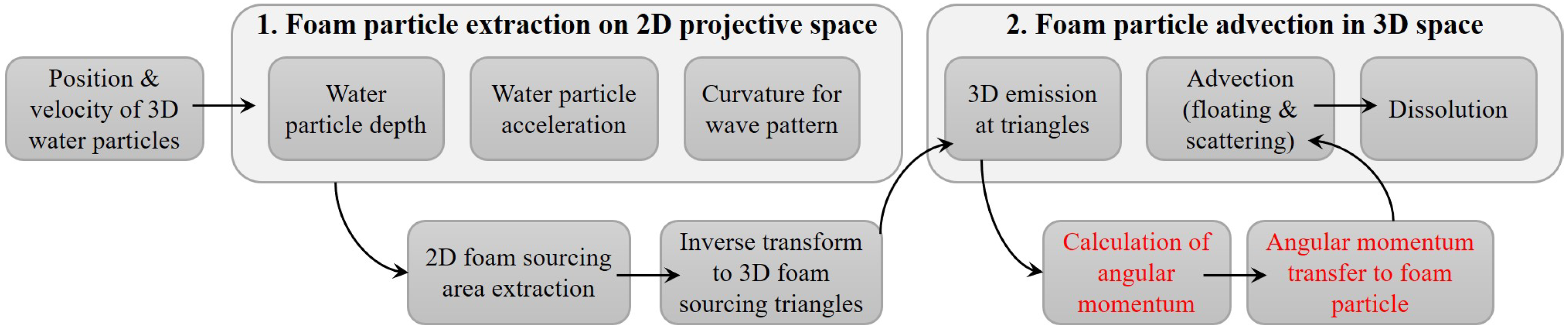
3. Proposed Framework

In this paper, the water particles are advected by calculating the underlying fluid simulation using the FLIP (Fluid-implicit particle) method, which is one of the hybrid methods using the particle-grid method. For foam generation, the previously proposed screen-space projection technique is used. The basic foam generation method is briefly reviewed in Section 3.1, and then the proposed method is explained in detail. A list of symbols is available in

Table 1. Simulation variables and parameters.

Name	Description	Value
r	Radius of water particle	–
$\mathbf{Z}$	Depth map	–
$\mathbf{D}$	Acceleration map	–
$\mathbf{P}$	Projection matrix	–
$\mathbf{Q}$	Inverse projection matrix	–
$x_p,y_p,z_p$	Projected coordinate	–
$r_x,r_y,r_z$	Projected radius	–
$d_p$	Projected acceleration	–
$\mathbf{C}$	Candidate region in 2D	–
${\mathbf{C}}^{*}$	Final candidate region in 2D	–
$\mathbf{F}$	Depth map based curvature	–
${\tau }_p$	Torque of water particle	–
${\mathbf{L}}_p$	Angular momentum of water particle	–
${\mathsf{\omega }}_p$	Angular velocity of water particle	–
$I_p$	Scalar inertia moment of water particle	–
${\mathsf{\omega }}_{pf}$	Relative angular velocity of water and foam particles	–
$H^{*}$	Mean curvature of the depth map	–
$\Delta$ t	Time-step	0.006
$\alpha$	Angular momentum transfer	10.0
$\beta$	Curvature threshold	0.1
k	Weight for inertia moment	$\frac{1}{30}$
h	Projective spacing	2.0
$N_x\times N_y$	Projective space res.	400 × 300

. The algorithm overview presented in this paper is depicted in Figure 3. The first step analyzes/extracts the flow from the two-dimensional space, while the second step advects the foam using angular momentum. The algorithm proposed in this paper is executed in the following order:

• Water particles advected using FLIP are projected onto screen-space through a projection matrix. Acceleration and depth values, which are physical quantities of water particles, are projected at the projected location.
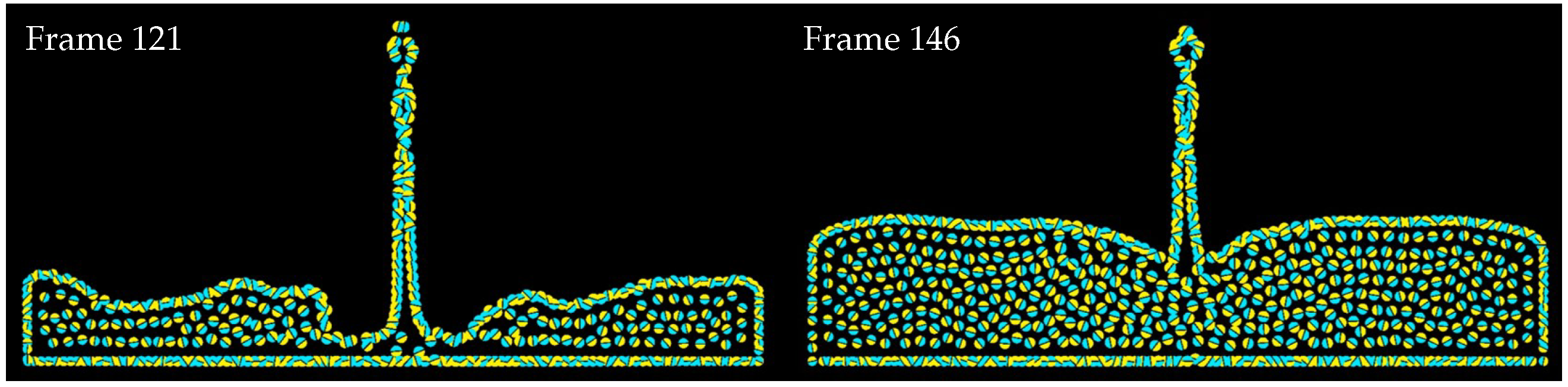
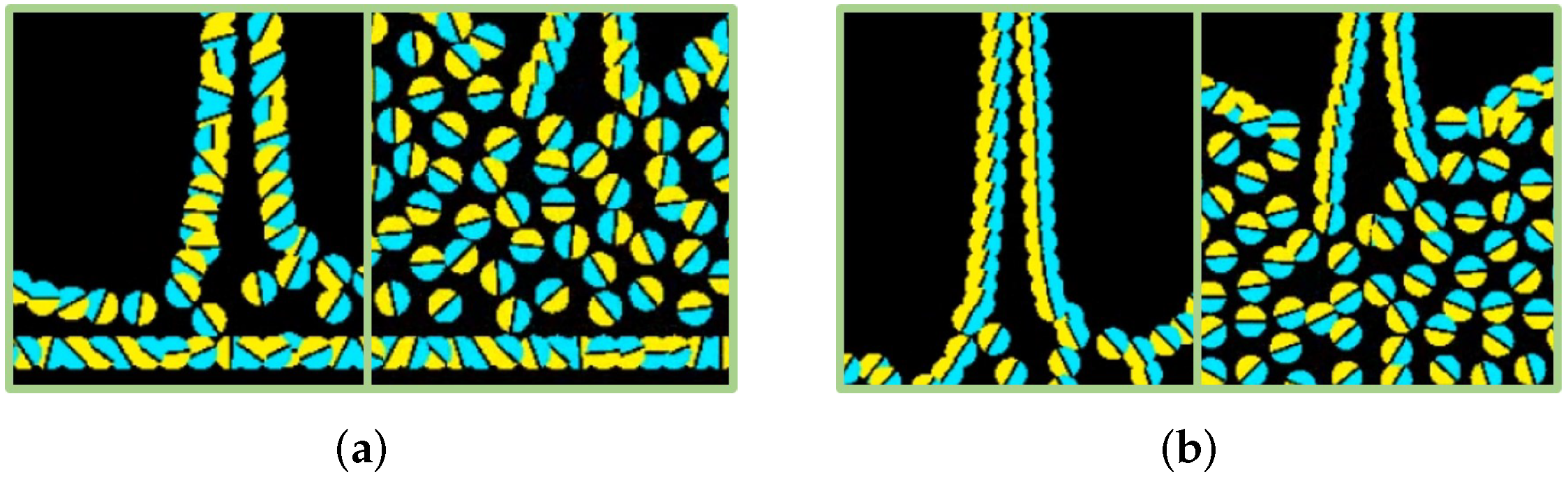
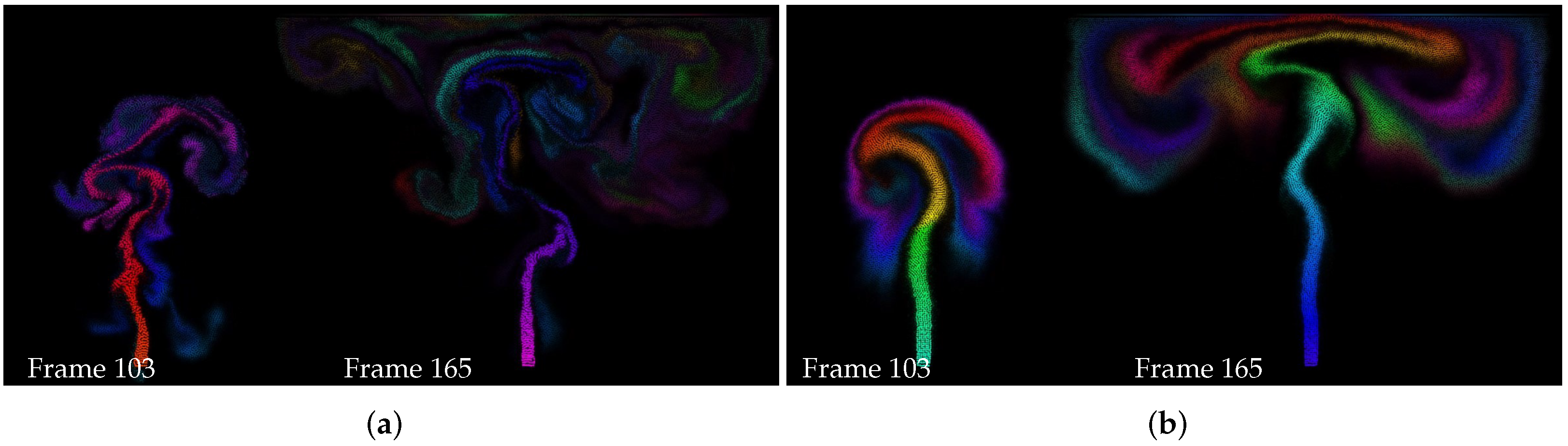
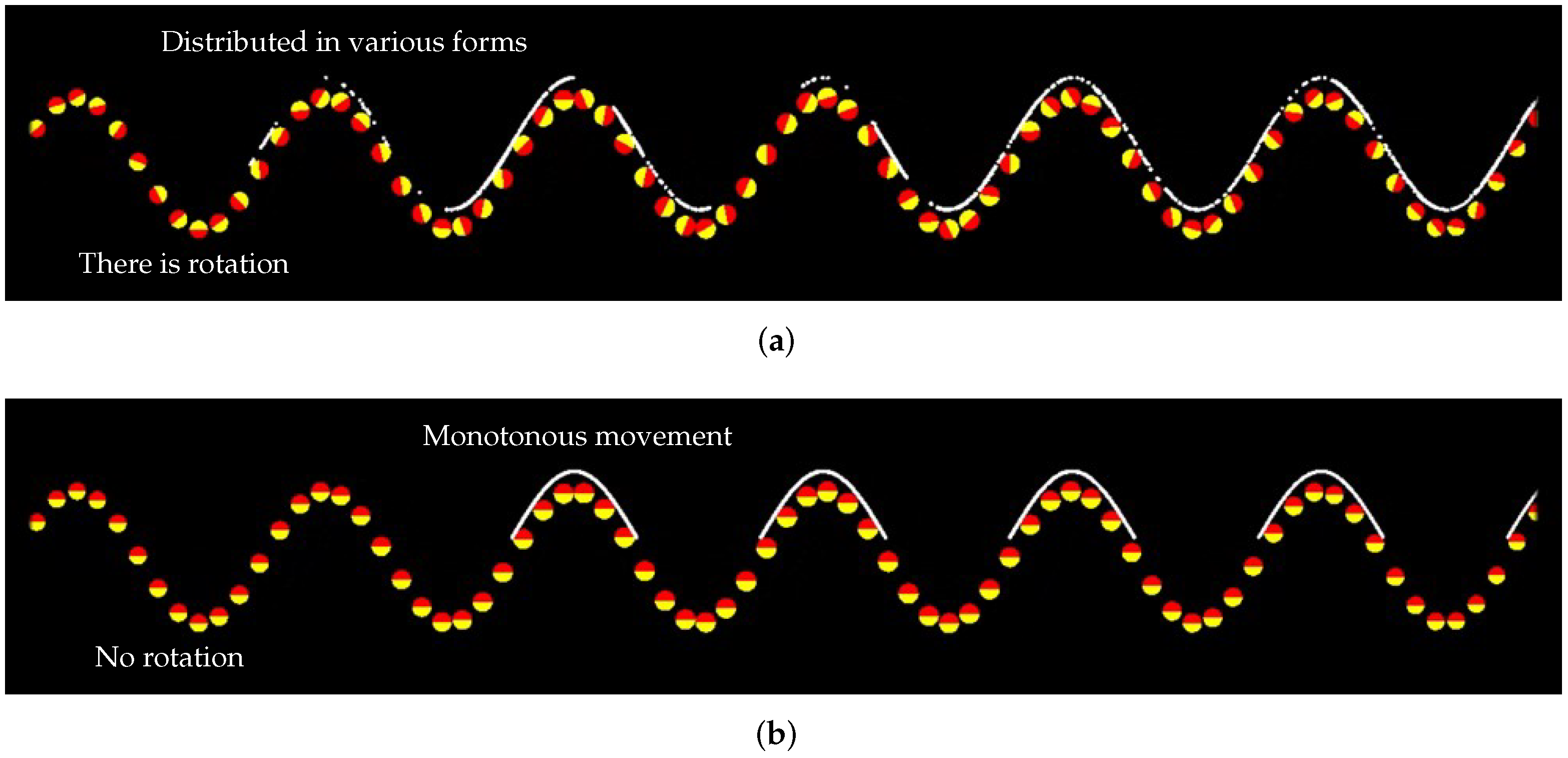
• The angular momentum is calculated from the water particles. In general particle-based simulation, since particles do not have volume or directionality, changes in angular momentum due to torque are not considered. We model this force and use it to advect the foam particles.
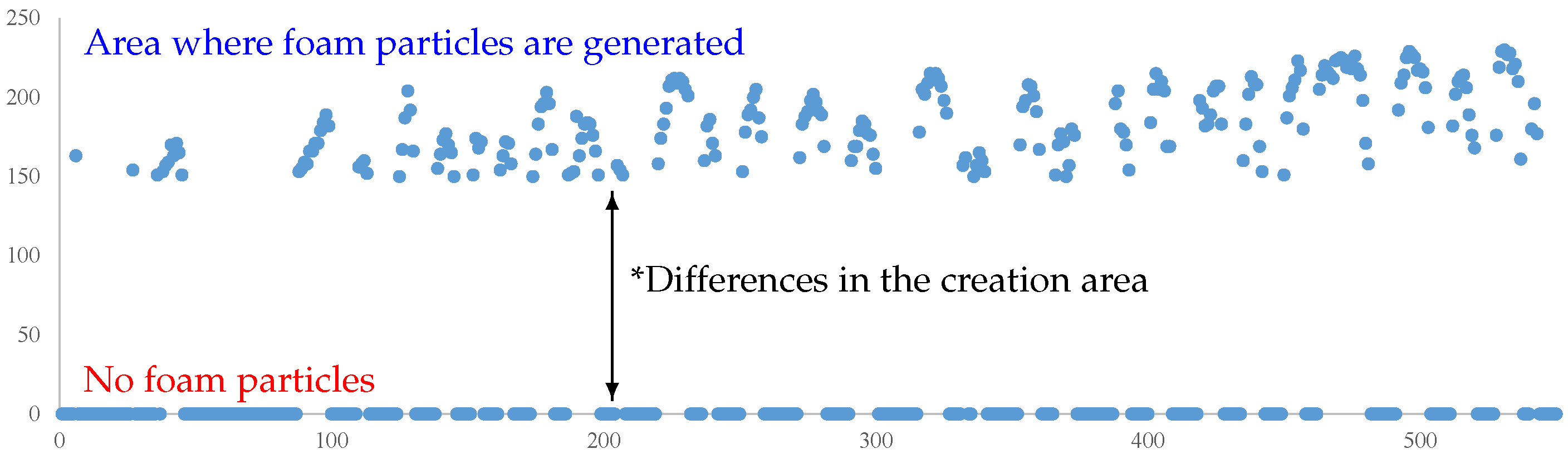
• Using the projected acceleration map, the place where the foam particles will be generated is quickly searched in 2D screen-space.
• Through inverse transformation from screen-space to 3D space, foam particles are generated in 3D space and advected based on angular velocity.
• Some foam particles are removed based on their lifespan or momentum.

3.1. Foam Effects Based on Projective-Space

3.1.1. Projection Map Generation from Fluid Particles

This section briefly describes the projective-space-based foam generation technique used in this paper. First, water particles in 3D space are projected onto screen space, and two maps are created that store the acceleration and depth values at the projected location, respectively. The meaning of each symbol in the following explanation is as follows: W and H are the horizontal and vertical pixel resolutions of the screen-space, respectively, $N_x\times N_y$ is the resolution of the regular grid divided by the projection interval h, and r is the radius of the water particles. r is a user-adjustable value to get a map where the values run smoothly after projection. As mentioned above, $z_{ij}$, which is the depth value of the water particles, and $d_{ij}$, which is the acceleration, are stored at the projected location, respectively, and each map is composed as follows: depth map $\mathbf{Z}\in {\mathbb{R}}^{N_x\times N_y}$, acceleration map $\mathbf{D}\in {\mathbb{R}}^{N_x\times N_y}$. The acceleration $d_{ij}$ of the water particle is calculated from the difference in velocity between frames: $\frac{|{\mathbf{v}}_{t+\Delta t}-{\mathbf{v}}_t|}{\Delta t}$.

A particle $\mathbf{x}$ at 3D location ${[x,y,z,1]}^T$ is projected onto 2D space using the projection matrix $\mathbf{P}$ (see Equation (1)).

$$\left[\begin{array}{c}{x}^{\prime }\\ y^{\prime }\\ z^{\prime }\\ w\end{array}\right]=\mathbf{P}\left[\begin{array}{c}x\\ y\\ z\\ 1\end{array}\right]$$

(1)

To avoid distortion of z values during projection, perspective division is applied only to the x and y coordinates. Using this method, the coordinates $(x_p,y_p),z_p$ where the 3D fluid particle is projected and the projected acceleration $d_p$ are calculated (see Equation (2)).

$$\underset{projectedcoordinatesanddepth}{\underbrace{\left[\begin{array}{c}{x}_p\\ y_p\\ z_p\end{array}\right]=\left[\begin{array}{c}W·\left(\frac{1}{2}+\frac{1}{2}{x}^{\prime }/w\right)\hfill \\ H·\left(\frac{1}{2}+\frac{1}{2}{y}^{\prime }/w\right)\hfill \\ z^{\prime }\hfill \end{array}\right]}},\underset{acceleration}{\underbrace{\left[\begin{array}{c}{x}_d\\ y_d\\ d_p\end{array}\right]=\left[\begin{array}{c}{x}_p\hfill \\ y_p\hfill \\ d\hfill \end{array}\right]}},$$

(2)

where $(x_d,y_d)$ is the index of the array in which $d_p$, the acceleration on screen space, is stored. The radius r of a particle in 3D space is projected using the following method (see Equation (3)):

$$\left[\begin{array}{c}{r}_x\\ r_y\\ r_z\end{array}\right]=\left[\begin{array}{c}rW\sqrt{p_{1,1}^2+p_{1,2}^2+p_{1,3}^2}/w\hfill \\ rH\sqrt{p_{2,1}^2+p_{2,2}^2+p_{2,3}^2}/w\hfill \\ r\sqrt{p_{3,1}^2+p_{3,2}^2+p_{3,3}^2}\hfill \end{array}\right],$$

(3)

where $p_{i,j}$ is an element of the projection matrix $\mathbf{P}$. Both $r_x$ and $r_y$ were set to $r_p$ to obtain isotropically projected radius values. There are three radius values in 3D and two in 2D via the projection step; in this paper, the $r_x$ value is used to obtain the isotropically projected radius value, and using the $r_y$ value is not a problem. What matters is that we use a single radius value to represent isotropic property. Based on the virtual camera settings used to compose the 3D scene, the projection matrix is constructed as a 4 × 4 matrix. Because this procedure follows the basic graphics pipeline used by OpenGL and Direct3D libraries, specific explanations are omitted.

Since a large number of fluid particles can be projected on the same node in screen space, the depth and acceleration values are updated as follows (see Equation (4)):

$$z_{ij}\leftarrow min(z_{ij},z_p-r_z{h}_{ij}),d_{ij}\leftarrow argmin\left(z_{ij}\right)$$

(4)

where

$$h_{ij}=\sqrt{1-\frac{{(ih-x_p)}^2+{(jh-y_p)}^2}{r_p^2}}$$

(5)

In the above equation, ${(ih-x_p)}^2+{(jh-y_p)}^2\le r_p^2$ is a condition for checking whether the projected coordinate is affected by other nodes in the projection space. As the depth buffer works, if $z_p-r_z{h}_{ij}$, which is the depth value of the projected coordinates, is smaller than $z_{ij}$, $z_{ij}$ and $d_{ij}$ are updated using Equation (4). An example of the acceleration map can be seen in Figure 4. (i, j) is the grid index in screen space. As shown in Table 1, the screen space in this paper is composed of a grid with a resolution of 400 × 300, and (i, j) in Equation (5) is the grid index near the projected location of the particle ($x_p$, $y_p$).

3.1.2. Foam Particle Generation

In this section, we extract 2D candidate regions where foam can be generated using the projection map described above (see Equation (6)).

$$\mathbf{C}=\left\{(i,j,k)|d>\gamma ,z\in \mathbf{Z},d\in \mathbf{D},(i,j)\in {\mathbb{R}}^{N_x\times N_y}\right\},$$

(6)

where $\gamma$ is the threshold used to find the fast flow region, and in this paper, it is set to 0.0001. $\mathbf{Z}$ and $\mathbf{D}$ are the depth and acceleration maps obtained through projection. If the $\gamma$ value is reduced, foam is generated even in the slow flow region, and the user can easily control the amount of foam generated by using this value. The ‘Marching Squares’ algorithm [38] was used to triangulate the extracted 2D foam area, and as a result, the candidate group of foam particles consists of 2D triangles. These triangles are transformed into 3D space through the inverse transformation of Equations (1) and (2). The coordinates of the transformed triangle are calculated with Equation (7).

$$\left[\begin{array}{c}x\\ y\\ z\\ 1\end{array}\right]=\mathbf{Q}\left[\begin{array}{c}(-1+2x_p/W)w\\ (-1+2y_p/H)w\\ z_p\\ w\end{array}\right],$$

(7)

where

$$w=\frac{1-q_{4,3}{z}_p}{q_{4,1}(-1+2x_p/W)+q_{4,2}(-1+2y_p/H)+q_{4,4}},$$

(8)

where $q_{i,j}$ is an element of the inverse projection matrix $\mathbf{Q}$, and as mentioned earlier, perspective division does not apply to $z_p$ [38]. The number of foam particles is determined based on the Weber number. (It is recommended to read the paper of Kim et al. [26,27] for more details.)

The next step is to calculate the wave pattern of the foam using the refined projection map. First, we calculate flow-based curvature in the projected space using the method proposed by Van der Lann et al. [36] (see Equation (9)).

$$\frac{\partial z}{\partial t}=H^{*},$$

(9)

Here, t is the time-step, and $H^{*}$ is the mean curvature of the depth map calculated in the 2D projection space. The depth map used in this process is $\mathbf{Z}$. Since the method of Van der Lann et al. [36] contains a noise pattern, it is necessary to repeatedly calculate the curvature in order to weaken it. Since this method erases the change pattern of the original curvature, in this paper, the wave pattern of the foam is calculated by modifying Equation (6) as Equation (10).

$${\mathbf{C}}^{*}=\left\{(i,j,k)|d>\gamma \cap f>\beta ,f\in \mathbf{F},(i,j)\in {\mathbb{R}}^{N_x\times N_y}\right\},$$

(10)

where $\mathbf{F}$ is the curvature of the depth map, and $\beta$ is a threshold value for finding a high curvature region, which is set to 0.1 in this paper. For advection of foam particles, the grid velocity field and water particles calculated through FLIP were used. In this process, Kim and Lee’s approach [26,27] was used as it is. (It is recommended to read the paper for a more detailed explanation.)

3.2. Angular Momentum of Water Particle and Advection of Foam Particle

In general, when a force is applied to an object with mass, a change occurs in the linear momentum of the object, and a torque is applied to an object with a volume depending on the point where the force is applied, resulting in a change in angular momentum. In most particle-based fluids, the change in angular momentum due to torque is not considered because particles do not have volume and directionality. The absence of angular momentum affects secondary effects that depend on the motion of the underlying fluids, causing viscous motion. In this paper, the angular momentum of water particles is modeled by converting the force acting on the neighboring water particles into a torque that affects the rotation of the particles. The calculated angular momentum is advected by the particles and designed to affect the foam particles. Angular motion through water particles is delivered to the foam particles in the following order:

• The force calculated by the neighbor water particles is converted into a torque acting on the particles. The calculated rotation momentum is integrated with time to maintain rotation.
• The rotation momentum of the water particles is applied to the force of the foam particles and incorporated into the advection process.

3.2.1. Angular Momentum Calculation in Fluid Particles

Rotational momentum is generated by the torque($\tau$ = $\mathbf{r}\times \mathbf{f}$) due to the difference in position($\mathbf{r}$) between the point of action of the force($\mathbf{f}$) acting on the object and the center of the mass of the object. However, since the point of action of the force applied to the water particles is the position of the particle, it has been considered to generate only linear momentum without angular momentum. In this paper, it is assumed that the force applied to the neighbor particle becomes the torque of the given particle, and the obtained torque is as Equation (11).

$${\tau }_p=\sum _{np}(({\mathbf{x}}_p-{\mathbf{x}}_{np})\times {\mathbf{f}}_{np})W_{p,np}$$

(11)

where ${\tau }_p$ is the torque applied to the particle. ${\mathbf{x}}_p$ and ${\mathbf{x}}_{np}$ are the positions of a given particle and its neighbor particle, $W_{p,np}$ is the smoothing weight function of the two water particles, and ${\mathbf{f}}_{np}$ is the force acting on the neighbor particle. × is a cross product operator. We calculated the torque acting on the water particle using Equation (11), and based on this, we update the angular momentum of the water particle by integrating with time as Equation (12).

$${\mathbf{L}}_p^{n+1}={\mathbf{L}}_p^n+{\tau }_p^n\Delta t$$

(12)

where ${\mathbf{L}}_p$ is the angular momentum of the water particle, and $\Delta t$ is the time-step. The angular velocity of the water particle is calculated with Equation (13).

$${\mathsf{\omega }}_p=I_p^{-1}{\mathbf{L}}_p^{n+1}$$

(13)

where ${\mathsf{\omega }}_p$ is the angular velocity of the water particle, and $I_p$ is the scalar inertia moment of the particle. In this paper, the inertia moment was calculated by approximating $I_p=k{m}_p$, and the value of $k=\frac{1}{30}$ was used.

3.2.2. Angular Momentum Transfer to Foam Particles

The angular momentum of the water particles calculated earlier should affect the momentum of the foam particles so that they rotate. To calculate the amount of change in the linear momentum of the foam particle due to angular momentum, we calculate the relative angular velocity between the water particle and the foam particle with Equation (14).

$${\mathsf{\omega }}_{pf}=\frac{({\mathbf{x}}_f-{\mathbf{x}}_p)\times ({\mathbf{v}}_f-{\mathbf{v}}_p)}{|{\mathbf{x}}_f-{\mathbf{x}}_p{|}^2}$$

(14)

where ${\mathsf{\omega }}_{pf}$ is the relative angular velocity of the foam particle around the water particle. ${\mathbf{x}}_f$ and ${\mathbf{x}}_p$ are the positions of foam particle and water particle, respectively, and ${\mathbf{v}}_f$ and ${\mathbf{v}}_p$ are the velocities of foam particle and water particle. In order for the angular velocity of the water particles to affect the linear momentum of the foam particles, we update the velocity of the foam particles as Equation (15).

$${\mathbf{v}}_f^{n+1}={\mathbf{v}}_f^{*}+\alpha \sum _p\left({\mathsf{\omega }}_p-{\mathsf{\omega }}_{pf}\right)\times ({\mathbf{x}}_f-{\mathbf{x}}_p)W_{pf}$$

(15)

where ${\mathbf{v}}_f^{*}$ is the velocity of the foam particle before angular motion is applied, and $W_{pf}$ is the isotropic weighting function between the foam particle and the water particle. $\alpha$ is the angular momentum transfer constant of the water particle, and in this paper, it is set to 10. Equation (15)’s aim is to transfer the water particle’s angular velocity (${\mathsf{\omega }}_p$) to the foam particle’s linear motion. As a result, the difference in angular velocity was utilized to induce the foam particle’s relative angular velocity (${\mathsf{\omega }}_{pf}$) to the water particle’s relative angular velocity (${\mathsf{\omega }}_p$).

3.2.3. Dissolution

The lifespan approach is used as a condition to remove the foam particles. The lifespan was maintained by accumulating the momentum of the foam particles in every frame, and the foam particles with a lifespan below the user-defined threshold were deleted. Recently, Kim and Lee proposed a method for efficiently reducing foam particles using a screen density calculated using the number of foam particles [26]. This method can be an add-on to our approach and is recommended for efficient reduction of foam particles.

4. Implementation

This study was implemented in the following environment: Intel i7-7700k 4.20 GHz. CPU 32 GB RAM, and NVIDIA GeForce GTX 1080 Ti graphics card. A FLIP-based fluid solver was used as the underlying water simulation, and a GPU-based preconditioned conjugate gradient method was used as a numerical matrix solver to calculate the fluid pressure. All momentum was stored in a FLIP grid using the ’Staggered Marker-and-Cell’ method [39], and the boundary particle method [40] proposed by Akinci et al. was used to handle the collision between fluid and solid.

In this paper, the particles were rendered by ray-tracing without reconstructing the surface of the fluid. The color of the water particles was set to (0.8, 0.5, 0.3), the color of the foam particle was set to (1.0, 1.0, 1.0), and the alpha value was used as 0.07. Each particle is projected into the image space to be rendered, and the pixels within a 3 × 3 range around the projected position are updated with Equation (16).

$$p_{i,j}=\left\{\begin{array}{c}{p}_{i,j}^r\leftarrow c_a{c}_r+(1-c_a)p_{i,j}^r\\ p_{i,j}^g\leftarrow c_a{c}_g+(1-c_a)p_{i,j}^g\\ p_{i,j}^b\leftarrow c_a{c}_b+(1-c_a)p_{i,j}^b\end{array}\right.,$$

(16)

where ($p_{i,j}^r,p_{i,j}^g,p_{i,j}^b$) is the pixel color, ($c_r,c_g,c_b$) is the particle color projected onto the image space, and $c_a$ is the alpha value.

There are three radius values in 3D and two in 2D via the projection step; in this paper, the $r_x$ value is used to obtain the isotropically projected radius value, and using the $r_y$ value is not a problem. What matters is that we use a single radius value to represent isotropic property.

Based on the virtual camera settings used to compose the 3D scene, the projection matrix is constructed as a 4 × 4 matrix. Because this procedure follows the basic graphics pipeline used by OpenGL and Direct3D libraries, specific explanations are omitted.

5. Results and Discussion

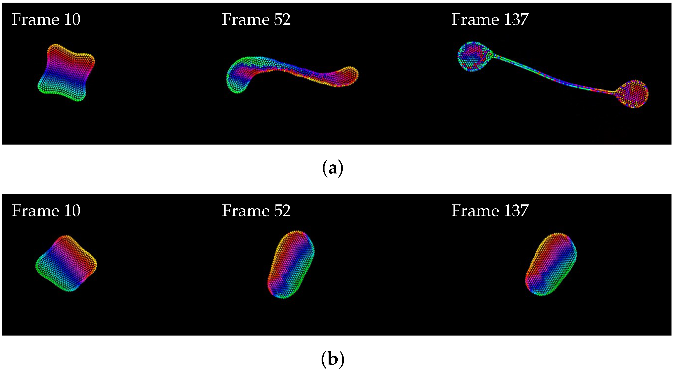
5.1. Validation Test for Angular Momentum

We conduct experiments in four scenarios to test the validation of the angular momentum method proposed in this paper.

In the first experiment, the angular momentum proposed in this paper was applied to rotational motion conversion (see Figure 5). The particles were placed in a normal distribution in 2D space, and initial velocity and angular velocity were applied. In order for the particle to rotate, the initial velocity of the particle, ${\mathbf{v}}_p^0$, was set as follows according to the relative position based on ${\mathbf{x}}_0$, the center of mass of the area where the particles are distributed: ${\mathbf{v}}_p^0=({\mathbf{x}}_0-{\mathbf{x}}_p)\times {\mathsf{\omega }}_0$ where ${\mathsf{\omega }}_0$ is the initial angular velocity and was set to $(0,0,10)$ in the above experiment. The experiment in Figure 5a shows the result when all particles move with angular velocity ${\mathsf{\omega }}_p={\mathsf{\omega }}_0$, and the experiment in Figure 5b shows the general particle-based fluids. In Figure 5a, as the particles continue to rotate while maintaining their initial rotation momentum, the region is separated by centrifugal force, and it is confirmed that the rotation momentum of the separated region is also maintained. In Figure 5b, it can be seen that the rotation momentum gradually weakens.

Second, we tested the rotational motion of particles in a particle-based water simulation (see Figure 6). In the falling water scene, rotational motion expressed when water particles interact with each other was observed. In the figure, the particle color is set to easily recognize the rotational motion, and when the falling water particles interact, it can be seen that the rotational motion is strongly expressed in the swaying area. Figure 7 shows a close-up of the part where the particles interact. In Figure 7b, the rotational motion of particles is hardly expressed, whereas in Figure 7a, our method well expresses the particle rotation by angular momentum that appears in the process of the particles interacting with each other. This rotational motion also affects the foam particles, improving the detail of secondary effects.

In the third scenario, we tested the rotational motion of particles in a particle-based smoke simulation with buoyancy force (see Figure 8). It was designed to source smoke particles after filling the simulation space with ghost particles. The smoke particle color is expressed by diffusing the color instead of the smoke density in a way that diffuses to nearby smoke and ghost particles, and the SPH gradient kernel (∇W) is used. Position-based fluids [11] were used as the basic algorithm.

In the fourth scenario, a two-dimensional experiment was conducted to check whether the intrinsic patterns of foam particles were well expressed by the angular momentum we proposed (see Figure 9). The movement of the water particles was controlled by the wave function, and the experiment was conducted based on the same distribution of foam particles. The wave function to move the water particles is as Equation (17)).

$$\left(x_i,y_i\right)\leftarrow \left(x_{i0}+v_0^{x}t,y_{0}sin\left(2\pi \frac{x}{{\lambda }_0}\right)cos\left(2\pi f_{0}t\right)\right)$$

(17)

where $v_0^x$ is the velocity of the wave, and $x_{i0}$ is the initial X-axis coordinate of the water particle. ${\lambda }_0$ is the wave length and $f_0$ is the wave frequency. Both experiments are based on the same wave and there is only difference in the presence or absence of angular momentum. For this experiment, the initial angular momentum of the water particles was randomly set in the first frame, and the water particles were designed to move while its value was maintained.

As can be seen from the experimental results, if angular momentum is not applied, the foam particles only follow the motion of the water particles, so a monotonous pattern that moves depending only on the water particles on the liquid surface appears (see Figure 9b). However, if angular momentum is applied to the advection of the foam particles, it can be confirmed that the foam particles continuously show dynamic movement due to the angular momentum of the water particles (see Figure 9a). In particular, the angular momentum is different according to the change in altitude such as wave crest, and this causes the foam particles to be dispersed in various shapes than in Figure 9b. Similar experimental results were also shown in Figure 2. As shown in Figure 2, different intrinsic patterns are created depending on the location of the foam particles. However, while the previous methods are static methods like a mask map that does not consider the motion of water, our method reflects the motion of water better. This characteristic is more evident in the animation of successive frames than in single frame.

In the 2D validation test shown earlier, the position of water particles was updated using angular velocity to show the effect of angular momentum. The angular momentum technique proposed in this paper reliably expresses the rotational motion of particles in various scenarios. In the next section, it can be seen that the turbulent flow of the foam is improved by applying angular momentum to the foam advection process.

5.2. Foam Effects with Angular Momentum

Three scenarios were devised to analyze the angular momentum-based foam advection technique proposed in this paper under various conditions. Based on these scenarios, the quality of foam effects using our method was compared with Kim and Lee’s method, which is a recent foam effects technique.

First, as a simple test scenario to prove the superiority of the proposed technique, a scene in which water particles are sourced was produced. In this scene, the time-step was set to 0.006 and more than 200,000 water particles were used. Figure 10 is a foam simulation using the method of Kim and Lee [26]. When the sourced water particles interact with the still water surface, angular momentum is strongly generated and rotational motion appears in the foam particles as well. This phenomenon is similarly shown in Figure 7, and the motion in which the foam particles are rolled more strongly by angular momentum compared to the previous technique is well expressed (see $\mathbf{A}$ in Figure 10a). As shown in $\mathbf{B}$ to $\mathbf{D}$, most of the angular motions were expressed well, and in the wave crest (the highest part of a wave, see Figure 11), remarkably lively foam particle motion was expressed.

Figure 12 is a scene where two boxes stir water, and foam effects are naturally created according to the movement path of the box. Due to the interaction of the water particles and the box, the vortex motion was clearly conveyed to the foam effects (see $\mathbf{A}$ and $\mathbf{B}$ in Figure 12). Additionally, as shown in $\mathbf{C}$ to $\mathbf{E}$, the wave crest created by the interaction of water particles clearly shows the motion as if the foam particles are being rolled in. As a result, compared to the previous method that expressed foam effects in an over-cloudy manner due to viscous foam particles, our method expressed the foam effects lively and showed clear foam patterns.

Figure 13 is the foam effects that appear when an external force in the form of tornado is added. If the previous results were generated by the sourcing of water particles or the impact of the solid, Figure 13 is the foam effects that are expressed due to the external force that is gradually strengthened. In addition, we examined how angular momentum affects the foam effects by using an external force of an unusual form such as tornado. In the 38th and 53rd frames of Figure 13a showing the gradual rotation, our technique expressed the foam effects symmetrically, whereas the previous technique did not reflect the angular momentum, so the effect of the tornado force was not well shown.

Figure 14 shows the foam effects created by the interaction of water particles inside the U-shaped corridor. In this figure, the blue region is where there is no angular momentum, and as the color goes from green to red, the angular momentum becomes stronger. It can be seen that the angular momentum of the foam particles is also strongly expressed as the water is bent into a curved shape by the interaction between the water particles and the wall (see $\mathbf{A}$ in Figure 14). As mentioned earlier, angular momentum was strong in the wave crest (see $\mathbf{B}$ and $\mathbf{C}$ in Figure 14), and foam particles that simply bounce into the air like splashes have relatively weak angular momentum, so it can be seen that they are expressed in blue (see $\mathbf{D}$ in Figure 14).

Figure 15 shows the difference of foam effects with or without our method. The red particles are generated using the previous technique [26], and the white particles are generated by advection based on angular momentum. Although the results were made in the scenes of the same configuration, the difference in motion of the foam particles was clearly revealed.

We present a method to improve the detail of secondary effects without tuning the original water particles. There are various methods for modeling turbulent flow in the field of fluid simulation, but it is difficult to control secondary effects using them because they are focused only on expressing the details of the underlying fluids. To make the foam effects more turbulent, the motion of the underlying water had to be tuned, and in the process, the motion of the original water was changed, so it was not easy to control both the underlying water and the foam effects at the same time. As seen in the previous results, our method updated the force without affecting the position of the original water particles by integrating only the angular momentum from the original water particles, and the foam effects were expressed vividly by incorporating the force into the foam advection process.

Table 2. Size of our example scene (Water: water particles, Foam: foam particles, Solid: triangles of the solid, Grid res.: grid resolution).

Figures	Water	Foam	Solid	Grid Res.	Projective Space Res.	Projective Spacing
Figure 5	1 k	–	–	–	–	–
Figure 6	3 k	–	–	–	–	–
Figure 8	45 k	–	–	–	–	–
Figure 9	100	5000	–	–	–	–
Figure 10	2.5 m	3.1 m	–	${150}^3$	400 × 300	2.0
Figure 12	1.7 m	1.2 m	48	${150}^3$	400 × 300	2.0
Figure 13	1.7 m	3.5 m	–	${150}^3$	400 × 300	2.0
Figure 14	1.2 m	3.3 m	70	${150}^3$	400 × 300	2.0

shows the parameters used to produce the experimental results in this study.

6. Conclusions

In this paper, the turbulent flow expression of the foam effect was improved by proposing a technique for advection of the foam particles using the angular momentum of the water particles. We experimented with foam effects under various scenarios and confirmed that the detail was improved due to angular momentum-based advection compared to the latest technique.

As the angular momentum becomes stronger, the foam effects appearing increasingly cloudy in the previous method have been greatly improved by introducing our method. The user can express the surface foam by controlling the angular momentum according to the characteristics of the scene to be produced, but this is not a perfect solution. Another trick is to apply our method only to the wave foam particles where the foam patterns are clearly expressed, so that the angular momentum can be expressed while maintaining the surface foam effects. In the future, based on LOD (Level-of-detail), adaptive, and anisotropic characteristics, we will study a method to reduce the number of foam particles while minimizing the quality loss of turbulent flow.

References

1. Stomakhin, A.; Schroeder, C.; Chai, L.; Teran, J.; Selle, A. A material point method for snow simulation. ACM Trans. Graph. (TOG) 2013, 32, 1–10. [Google Scholar] [CrossRef]
2. Yue, Y.; Smith, B.; Batty, C.; Zheng, C.; Grinspun, E. Continuum foam: A material point method for shear-dependent flows. ACM Trans. Graph. (TOG) 2015, 34, 1–20. [Google Scholar] [CrossRef]
3. Zhu, Y.; Bridson, R. Animating sand as a fluid. ACM Trans. Graph. (TOG) 2005, 24, 965–972. [Google Scholar] [CrossRef]
4. Sato, T.; Wojtan, C.; Thuerey, N.; Igarashi, T.; Ando, R. Extended narrow band FLIP for liquid simulations. In Computer Graphics Forum; Wiley Online Library: Malden, MA, USA, 2018; Volume 37, pp. 169–177. [Google Scholar]
5. Nielsen, M.B.; Bridson, R. Spatially adaptive FLIP fluid simulations in bifrost. In ACM SIGGRAPH 2016 Talks; Association for Computing Machinery: New York, NY, USA, 2016; pp. 1–2. [Google Scholar]
6. Jiang, C.; Schroeder, C.; Selle, A.; Teran, J.; Stomakhin, A. The affine particle-in-cell method. ACM Trans. Graph. (TOG) 2015, 34, 1–10. [Google Scholar] [CrossRef]
7. Ding, O.; Shinar, T.; Schroeder, C. Affine particle in cell method for MAC grids and fluid simulation. J. Comput. Phys. 2020, 408, 109311. [Google Scholar] [CrossRef]
8. Fu, C.; Guo, Q.; Gast, T.; Jiang, C.; Teran, J. A polynomial particle-in-cell method. ACM Trans. Graph. (TOG) 2017, 36, 1–12. [Google Scholar] [CrossRef] [Green Version]
9. Müller, M.; Charypar, D.; Gross, M.H. Particle-based fluid simulation for interactive applications. In Proceedings of the 2003 ACM SIGGRAPH/Eurographics Symposium on Computer Animation, San Diego, CA, USA, 26–27 July 2003; pp. 154–159. [Google Scholar]
10. Becker, M.; Teschner, M. Weakly compressible SPH for free surface flows. In Proceedings of the 2007 ACM SIGGRAPH/Eurographics Symposium on Computer Animation, San Diego, CA, USA, 2–4 August 2007; pp. 209–217. [Google Scholar]
11. Macklin, M.; Müller, M. Position based fluids. ACM Trans. Graph. (TOG) 2013, 32, 1–12. [Google Scholar] [CrossRef]
12. Chen, F.; Zhao, Y.; Yuan, Z. Langevin Particle: A Self-Adaptive Lagrangian Primitive for Flow Simulation Enhancement. In Computer Graphics Forum; Blackwell Publishing Ltd.: Oxford, UK, 2011; Volume 30, pp. 435–444. [Google Scholar]
13. Zhao, Y.; Yuan, Z.; Chen, F. Enhancing Fluid Animation with Adaptive, Controllable and Intermittent Turbulence. In Symposium on Computer Animation; Eurographics Association: Madrid, Spain, 2010; pp. 75–84. [Google Scholar]
14. Yoon, J.C.; Kam, H.R.; Hong, J.M.; Kang, S.J.; Kim, C.H. Procedural synthesis using vortex particle method for fluid simulation. In Computer Graphics Forum; Blackwell Publishing Ltd.: Oxford, UK, 2009; Volume 28, pp. 1853–1859. [Google Scholar]
15. Weißmann, S.; Pinkall, U. Filament-based smoke with vortex shedding and variational reconnection. In ACM SIGGRAPH 2010 Papers; Association for Computing Machinery: New York, NY, USA, 2010; pp. 1–12. [Google Scholar]
16. Barnat, A.; Pollard, N.S. Smoke sheets for graph-structured vortex filaments. In Proceedings of the 11th ACM SIGGRAPH/Eurographics Conference on Computer Animation, Lausanne, Switzerland, 29–31 July 2012; pp. 77–86. [Google Scholar]
17. Kim, D.; Lee, S.W.; Song, O.y.; Ko, H.S. Baroclinic turbulence with varying density and temperature. IEEE Trans. Vis. Comput. Graph. 2011, 18, 1488–1495. [Google Scholar]
18. Hong, J.M.; Shinar, T.; Fedkiw, R. Wrinkled flames and cellular patterns. ACM Trans. Graph. (TOG) 2007, 26, 47-es. [Google Scholar] [CrossRef]
19. Kim, D.; Song, O.Y.; Ko, H.S. Stretching and wiggling liquids. In ACM SIGGRAPH Asia 2009 Papers; Association for Computing Machinery: New York, NY, USA, 2009; pp. 1–7. [Google Scholar]
20. Mercier, O.; Beauchemin, C.; Thuerey, N.; Kim, T.; Nowrouzezahrai, D. Surface turbulence for particle-based liquid simulations. ACM Trans. Graph. (TOG) 2015, 34, 1–10. [Google Scholar] [CrossRef]
21. Pfaff, T.; Thuerey, N.; Gross, M. Lagrangian vortex sheets for animating fluids. ACM Trans. Graph. (TOG) 2012, 31, 1–8. [Google Scholar] [CrossRef]
22. Pfaff, T.; Thuerey, N.; Cohen, J.; Tariq, S.; Gross, M. Scalable fluid simulation using anisotropic turbulence particles. In ACM SIGGRAPH Asia 2010 Papers; Association for Computing Machinery: New York, NY, USA, 2010; pp. 1–8. [Google Scholar]
23. Kim, T.; Thürey, N.; James, D.; Gross, M. Wavelet turbulence for fluid simulation. ACM Trans. Graph. (TOG) 2008, 27, 1–6. [Google Scholar]
24. Pfaff, T.; Thuerey, N.; Selle, A.; Gross, M. Synthetic turbulence using artificial boundary layers. In ACM SIGGRAPH Asia 2009 Papers; Association for Computing Machinery: New York, NY, USA, 2009; pp. 1–10. [Google Scholar]
25. Ihmsen, M.; Akinci, N.; Akinci, G.; Teschner, M. Unified spray, foam and air bubbles for particle-based fluids. Vis. Comput. 2012, 28, 669–677. [Google Scholar] [CrossRef]
26. Kim, J.H.; Lee, J. Synthesizing Large-Scale Fluid Simulations with Surface and Wave Foams via Sharp Wave Pattern and Cloudy Foam. Comput. Animat. Virtual Worlds 2021, 32, e1984. [Google Scholar] [CrossRef]
27. Kim, J.H.; Lee, J.; Cha, S.; Kim, C.H. Efficient representation of detailed foam waves by incorporating projective space. IEEE Trans. Vis. Comput. Graph. 2016, 23, 2056–2068. [Google Scholar] [CrossRef] [PubMed]
28. Takahashi, T.; Fujii, H.; Kunimatsu, A.; Hiwada, K.; Saito, T.; Tanaka, K.; Ueki, H. Realistic animation of fluid with splash and foam. In Computer Graphics Forum; Blackwell Publishing Ltd.: Oxford, UK, 2003; Volume 22, pp. 391–400. [Google Scholar]
29. Geiger, W.; Leo, M.; Rasmussen, N.; Losasso, F.; Fedkiw, R. So real it’ll make you wet. In ACM SIGGRAPH 2006 Sketches; Association for Computing Machinery: New York, NY, USA, 2006; p. 20-es. [Google Scholar]
30. Hieber, S.E.; Koumoutsakos, P. A Lagrangian particle level set method. J. Comput. Phys. 2005, 210, 342–367. [Google Scholar] [CrossRef]
31. Nishida, T.; Sugihara, K.; Kimura, M. Stable marker-particle method for the Voronoi diagram in a flow field. J. Comput. Appl. Math. 2007, 202, 377–391. [Google Scholar] [CrossRef] [Green Version]
32. Kim, J.; Cha, D.; Chang, B.; Koo, B.; Ihm, I. Practical animation of turbulent splashing water. In Symposium on Computer Animation; A K Peters/CRC Press: Natick, MA, USA, 2006; pp. 335–344. [Google Scholar]
33. Losasso, F.; Talton, J.; Kwatra, N.; Fedkiw, R. Two-way coupled SPH and particle level set fluid simulation. IEEE Trans. Vis. Comput. Graph. 2008, 14, 797–804. [Google Scholar] [CrossRef]
34. Mihalef, V.; Metaxas, D.; Sussman, M. Simulation of two-phase flow with sub-scale droplet and bubble effects. In Computer Graphics Forum; Blackwell Publishing Ltd.: Oxford, UK, 2009; Volume 28, pp. 229–238. [Google Scholar]
35. Wang, C.b.; Zhang, Q.; Kong, F.l.; Qin, H. Hybrid particle–grid fluid animation with enhanced details. Vis. Comput. 2013, 29, 937–947. [Google Scholar] [CrossRef]
36. van der Laan, W.J.; Green, S.; Sainz, M. Screen space fluid rendering with curvature flow. In Proceedings of the 2009 Symposium on Interactive 3D Graphics and Games; Association for Computing Machinery: New York, NY, USA, 2009; pp. 91–98. [Google Scholar]
37. Bagar, F.; Scherzer, D.; Wimmer, M. A layered particle-based fluid model for real-time rendering of water. In Computer Graphics Forum; Blackwell Publishing Ltd.: Oxford, UK, 2010; Volume 29, pp. 1383–1389. [Google Scholar]
38. Müller, M.; Schirm, S.; Duthaler, S. Screen space meshes. In Proceedings of the 2007 ACM SIGGRAPH/Eurographics Symposium on Computer Animation, San Diego, CA, USA, 2–4 August 2007; pp. 9–15. [Google Scholar]
39. Harlow, F.H.; Welch, J.E. Numerical calculation of time-dependent viscous incompressible flow of fluid with free surface. Phys. Fluids 1965, 8, 2182–2189. [Google Scholar] [CrossRef]
40. Akinci, N.; Cornelis, J.; Akinci, G.; Teschner, M. Coupling elastic solids with smoothed particle hydrodynamics fluids. Comput. Animat. Virtual Worlds 2013, 24, 195–203. [Google Scholar] [CrossRef]
Figure 1. Extracted wave patterns. The color of each pixel indicates the curvature value (red: high, blue: low). (a) Base water flow (red line: evaluation region, see Figure 2). (b) Intrinsic patterns of foam with Kim et al. [26,27].
Applsci 12 00133 g001
Figure 2. Curvature values at the evaluation region (see red line in Figure 1a).
Applsci 12 00133 g002
Figure 3. Algorithm overview.
Applsci 12 00133 g003
Figure 4. Acceleration map projected onto screen-space (red: fast acceleration, blue: slow acceleration, inset image: simulation view) (a) Frame 115. (b) Frame 243.
Applsci 12 00133 g004
Figure 5. Angular momentum in the process of rotation. The related video has been submitted as Supplementary Material. (a) With angular momentum (our method). (b) Without angular momentum.
Applsci 12 00133 g005
Figure 6. Two-dimensional water particle simulation with our method. The related video has been submitted as Supplementary Material.
Applsci 12 00133 g006
Figure 7. Comparison of close-up views in Figure 6. The related video has been submitted as Supplementary Material. (a) Our method. (b) Without angular momentum.
Applsci 12 00133 g007
Figure 8. Comparison of 2D particle-based smoke simulation results. The related video has been submitted as Supplementary Material. (a) Our method. (b) Without angular momentum.
Applsci 12 00133 g008
Figure 9. Comparison of movement and pattern change of foam particles. The related video has been submitted as Supplementary Material. (a) Our method. (b) Without angular momentum.
Applsci 12 00133 g009
Figure 10. Comparison of the rotating-emitter scene in water simulation. The related video has been submitted as Supplementary Material. (a) Our method. (b) Kim and Lee [26].
Applsci 12 00133 g010
Figure 11. Wave concepts.
Applsci 12 00133 g011
Figure 12. Rotating two boxes in water simulation. The related video has been submitted as Supplementary Material. (a) Our method (inset image: simulation view). (b) Kim and Lee [26].
Applsci 12 00133 g012
Figure 13. Tornado scene. The related video has been submitted as Supplementary Material. (a) Our method. (b) Kim and Lee [26].
Applsci 12 00133 g013
Figure 14. Foam effects by fluid–solid interaction using our method as the water flows along the U-shaped corridor (blue: no angular momentum, green to red: stronger angular momentum). The related video has been submitted as Supplementary Material.
Applsci 12 00133 g014
Figure 15. Motion difference with (white) or without (red) angular momentum-based advection. The related video has been submitted as Supplementary Material.
Applsci 12 00133 g015