STHarDNet: Swin Transformer with HarDNet for MRI Segmentation

Abstract

In magnetic resonance imaging (MRI) segmentation, conventional approaches utilize U-Net models with encoder–decoder structures, segmentation models using vision transformers, or models that combine a vision transformer with an encoder–decoder model structure. However, conventional models have large sizes and slow computation speed and, in vision transformer models, the computation amount sharply increases with the image size. To overcome these problems, this paper proposes a model that combines Swin transformer blocks and a lightweight U-Net type model that has an HarDNet blocks-based encoder–decoder structure. To maintain the features of the hierarchical transformer and shifted-windows approach of the Swin transformer model, the Swin transformer is used in the first skip connection layer of the encoder instead of in the encoder–decoder bottleneck. The proposed model, called STHarDNet, was evaluated by separating the anatomical tracings of lesions after stroke (ATLAS) dataset, which comprises 229 T1-weighted MRI images, into training and validation datasets. It achieved Dice, IoU, precision, and recall values of 0.5547, 0.4185, 0.6764, and 0.5286, respectively, which are better than those of the state-of-the-art models U-Net, SegNet, PSPNet, FCHarDNet, TransHarDNet, Swin Transformer, Swin UNet, X-Net, and D-UNet. Thus, STHarDNet improves the accuracy and speed of MRI image-based stroke diagnosis.

1. Introduction

Strokes pose a threat to human health because of their high incidence, mortality rate, and potential for causing disabilities. Strokes can be diagnosed using a variety of advanced testing methods, among which brain computed tomography (CT) or magnetic resonance imaging (MRI) are often used. The CT scan is the best method for classifying acute cerebral infarction and brain hemorrhage and is performed first in patients suspected of having strokes to determine initial treatment. In the case of cerebral infarction, it is displayed as a low density, and in the case of a stroke, it is displayed as high density. However, the infarction part does not appear well in the early stage of cerebral infarction. An MRI test is similar to a CT scan, but it has the advantage that it can accurately find small lesions or lesions in the brain region that are difficult to find in CT scans because it has much better imaging power. Many studies have been conducted on stroke diagnosis using computer vision technology to help doctors with diagnosis [1,2,3]. Conventional CT or MRI image-based diagnoses have often used U-Net models [4] with encoder–decoder structure using the convolution neural network (CNN) structure and obtained good results.

Recently, with the application of transformers to the computer vision field, many segmentation models using transformers have also been proposed [5,6]. A transformer is a successful example of applying the method of processing sequence data in natural language processing (NLP) analysis to the field of computer vision. Transformers currently exhibit good performance in the field of computer vision, including detection [7], segmentation [8], and classification [9]. Furthermore, models that have an encoder–decoder structure by combining a CNN model and a vision transformer (ViT) model have also performed well in medical image analysis [10,11]. Currently, many combination models of CNN and ViT use transformers in the bottleneck of the CNN-based encoder–decoder model so that parameters of the encoder and decoder can be delivered more effectively [12,13]. However, CNN-based encoder–decoder models are large in size and slow in terms of calculation speed, and ViT models have the problem that the calculation amount of the model increases sharply as the image size increases. One of the reasons why the transformer is used in the bottleneck in conventional combination models of CNN and ViT is to minimize the effect that the transformer has on the overall calculation speed as the size of the input feature map increases.

This study combines a HarDNet block [14], a lightweight model structure among CNN models, and a Swin Transformer model, which solves the problem of the calculation amount increasing sharply in the transformer model as the image size increases in the ViT model. This is to solve the existing problem and, at the same time, obtain high performance.

To this end, an encoder–decoder model in the form of U-Net is constructed with HarDNet blocks. Unlike a method that uses a transformer layer in the bottleneck of the encoder–decoder in past studies, this study uses a Swin Transformer [15] model in the first skip connection layer of the encoder model. As a result, the Swin Transformer model maintains the advantages of shifted windows approach based on self-attention and hierarchical feature extraction because a larger feature map is applied compared to when it is used in the bottleneck. The STHarDNet model proposed in this study has the following characteristics:

• Using HarDNet blocks, the proposed model improves slow computational speed, a disadvantage of the conventional CNN-based encoder–decoder structure model.
• Using the Swin Transformer, the proposed model solves the problem in which the memory use and computations increase as the image size increases in the ViT model.
• Using the first skip connection layer in the encoder of the Swin Transformer model in the encoder–decoder model that has the U-Net structure, it accepts a feature map larger than the bottleneck as input and maintains the Swin Transformer model’s shifted windows approach and hierarchical transformer characteristics.

This study used the Anatomical Tracings of Lesions After Stroke (ATLAS) to conduct comparative experiments of performance. The ATLAS dataset is a standardized open dataset built for performance comparison of various algorithms that manually segment lesion locations in the MRI images of 229 stroke patients. In the ATLAS data, the MRI images of 177 patients were used as training data, and the data of the remaining 52 patients were used as validation data to conduct the comparative experiments of performance with existing state-of-the-art (SOTA) models. In the results, the proposed model’s Dice, IoU, precision, and recall were 0.5547, 0.4185, 0.6764, and 0.5286, respectively, indicating that the proposed model performed better than the conventional model. Furthermore, it showed faster performance in the comparative calculation speed test of the models.

2. Related Work

2.1. HarDNet Block

The HarDNet Block consists of multiple harmonic dense blocks (HDBs). In the HarDNet Block, a depthwise-separable convolution layer is used for connection between HDBs. This reduced the convolutional input/output (CIO) by 50% compared to when a 1 × 1 convolutional layer and a 2 × 2 average pooling layer were used in DenseNet [14]. In the connection method between HDBs, when the value of $k-2^n$ is larger than 0, and the value of $\frac{2^n}{k}$ is a natural number, the $k$-th layer is connected to the $k-2^n$-th layer, as shown in Equation (1). In Equation (1), $k$ is the position of the layer in HDB, $n$ is the layer connected to $k$ in the HDB, and $N$ is a natural number.

$$C_k=k-2^n, if\hspace{1em}\frac{2^n}{k}\in N,\hspace{1em}k-2^n\ge 0$$

(1)

2.2. Swin Transformer Block

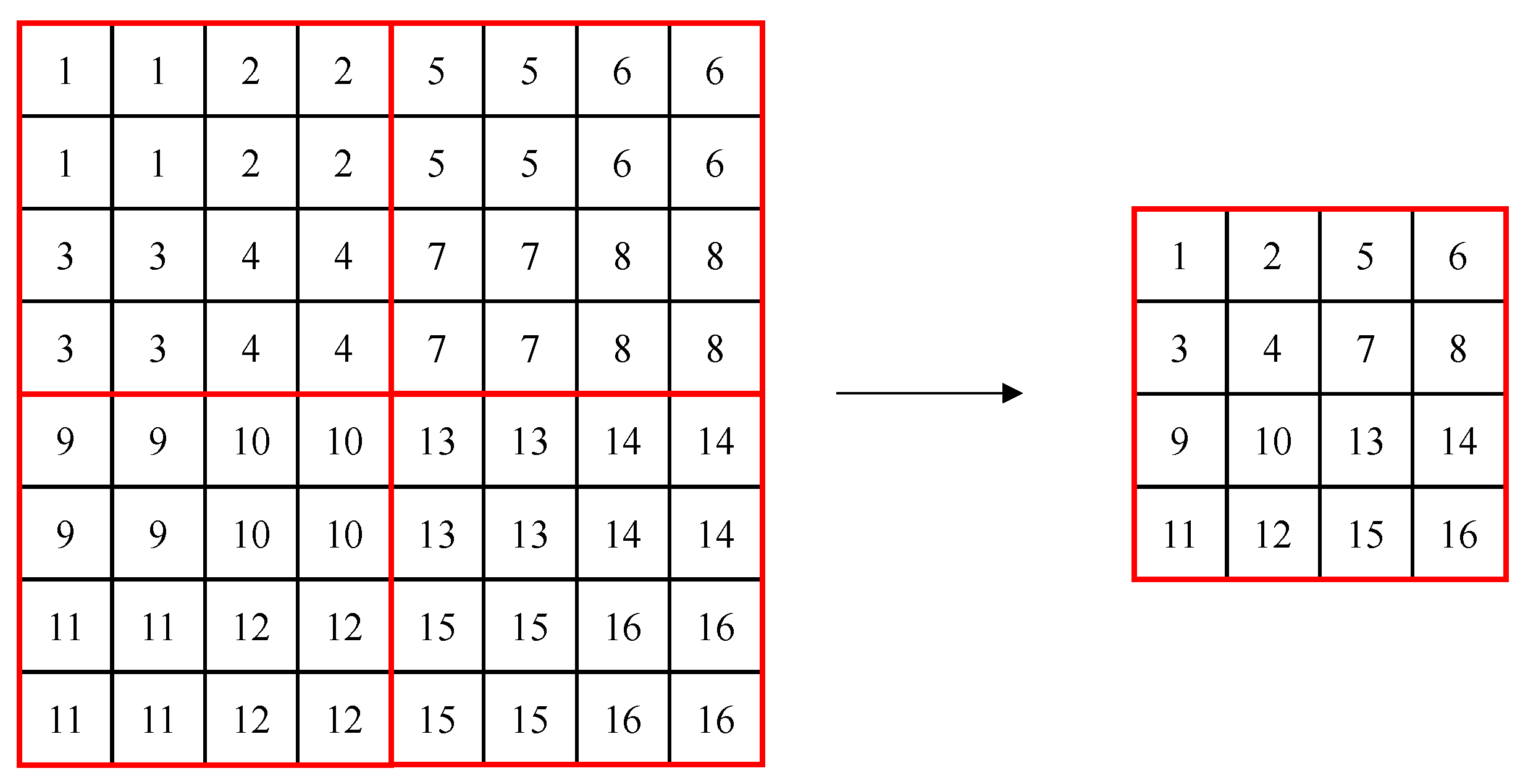
The Swin Transformer consists of Swin transformer blocks, which are created to be suitable for detection and segmentation by introducing the concept of a hierarchical feature map and shifted windows to ViT. In conventional transformers, self-attention is performed by creating tokens with the same patch size, but the Swin Transformer uses a method of merging adjacent patches gradually, starting from a patch size of 4 × 4, like the hierarchical structure of the feature pyramid network. This allows using each hierarchical feature map’s information, like U-Net. Figure 1 shows the patch merging process, where, in the figure, a red box refers to a window, the small box (1–16) refers to a patch (token) with a size of 4 × 4, and patch merging merges 2 × 2 patches into one. In the process of patch merging, the feature map’s size is down-sampled to (W/2, H/2).

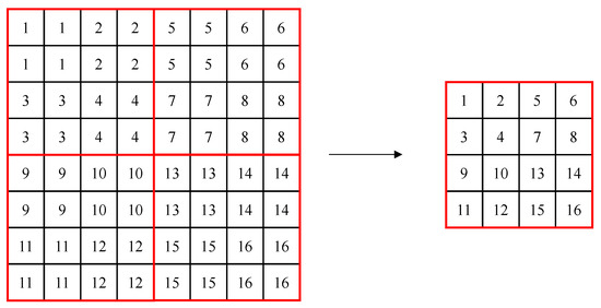
Figure 1. Example of patch merging in windows of the Swin Transformer.

For Swin transformer blocks, self-attention is performed in respective windows only, and merging is performed in the last feature map. This solves the problem of increasing computations when the image size increases in conventional ViT. However, the positions of the windows are fixed, and the relationship between the windows is not represented because self-attention is performed in the fixed windows only. Therefore, to calculate the relationship between two windows, the window is shifted to the right (→) and down (↓) directions by window size/2, and the self-attention is performed once more [15]. As a result, the Swin Transformer facilitates the analysis of the entire input image with self-attention alone in respective windows.

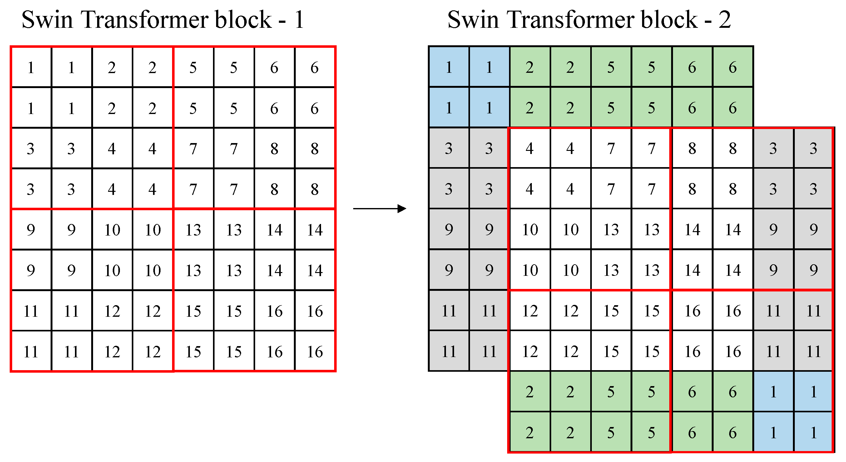
Figure 2 shows an example of the shifted windows approach. In Figure 2, a red box means a window, and a small box (1–16) means a patch (token) with a size of 4 × 4. In the figure, there are four windows with a window size of 4. In Swin transformer block 2, the windows are shifted based on Swin transformer block 1. In Swin transformer block 2, the windows are shifted in the right (→) and down (↓) directions by the window size/2, and the feature parts that the windows lack are supplemented, as shown in colors in the figure.

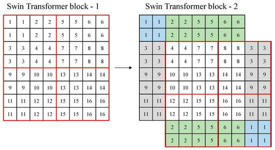
Figure 2. Example of a shifted window approach of the Swin Transformer.

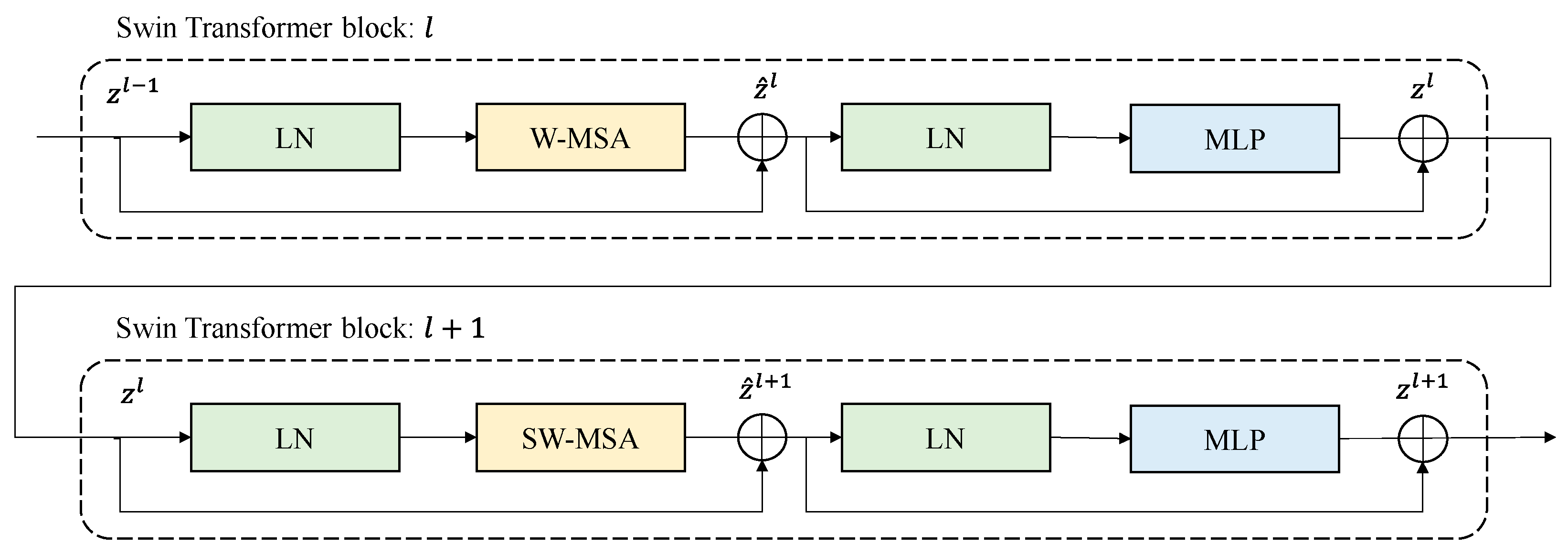
Figure 3 below shows a schematic diagram for connecting two Swin transformer blocks. As shown in the figure, the standard windows-based, multi-head, self-attention (W-MSA) module and shifted window-based, multi-head, self-attention (SW-MSA) module are used sequentially in the Swin transformer block. There is LayerNorm (LN) in front and back of S(W)-MSA, and the last MPL consists of two GELU non-linearities. Therefore, the Swin transformer block is used in multiples of two [16].

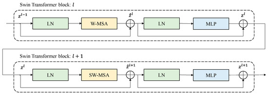
Figure 3. Examples of connections of the Swin transformer blocks.

Connections of Swin transformer blocks can be expressed in Equations (2)–(5) below, where ‘${\widehat{z}}^l$’ is the output of (S)W-MSA, ‘$z^l$’ is the output of MLP, and ‘$l$’ denotes the position of the Swin transformer block.

$${\widehat{z}}^l=W-MSA\left(LN\left(z^{l-1}\right)\right)+z^{l-1}$$

(2)

$$z^l=MLP\left(LN\left(\widehat{z}\right)\right)+{\widehat{z}}^l$$

(3)

$${\widehat{z}}^{l+1}=SW-MSA\left(LN\left(z^l\right)\right)+z^l$$

(4)

$$z^{l+1}=MLP\left(LN\left({\widehat{z}}^{l+1}\right)\right)+{\widehat{z}}^{l+1}$$

(5)

2.3. Past Studies on Models Constructed Based on the ATLAS Dataset

Qi et al. [17] proposed an X-Net with an encoder–decoder structure using 2D CNN to analyze the ATLAS data. The X-block used in X-Net consisted of three (3 × 3) depthwise-separable convolution layers, a 1 × 1 convolution layer, and one 1 × 1 convolution layer that connects input and output. The size of the input and output of X-Net was 224 × 192, and when training the model, the sum of Dice loss and cross-entropy loss was used in the loss function. In the experimental results using the five-fold cross-validation method with the ATLAS dataset, the following performances were obtained: a Dice of 0.4867, IoU of 0.3723, precision of 0.6, and recall of 0.4752.

Zhou et al. [18] proposed a dimension-fusion-UNet (D-UNet) of an encoder–decoder structure that combined 2D and 3D CNNs. Zhou et al. [2] combined four grayscale images into one 3D image, where the inputs of D-UNet were 192 × 192 × 4 in 2D form and 192 × 192 × 4 × 1 in 3D form. The output of D-UNet was 192 × 192 × 1, which was based on the ground truth value corresponding to the third MRI scan image in the four grayscale images used for the generation of a 3D image. D-UNet was trained using the MRI scan images of 183 patients in the ATLAS dataset and validated using the MRI scan images of 46 patients, obtaining a Dice of 0.5349.

Basak et al. [19] modified the CNN decoder in the D-UNet’s decoder into a parallel partial decoder (PPD) and the obtained performances were Dice, IoU, precision, and recall of 0.5457, 0.4015, 0.6371, and 0.4969, respectively. Zhang et al. [20] obtained good performance by preprocessing the ATLAS data using the large deformation diffeomorphic metric mapping (LDDMM) method and inputting them into U-Net. Furthermore, they compared the performance of 2D U-Net and 3D U-Net with the same dataset and obtained the following results: when the data without preprocessing was used, the Dice of 2D U-Net was 0.4554, and that of 3D U-Net was 0.5296; when the preprocessed dataset was used, the Dice of 2D U-Net was 0.4954, and that of 3D U-Net was 0.5672. Therefore, the model’s performance improved when the ATLAS data were preprocessed using the LDDMM method, and the performance of 3D U-Net was relatively better than that of 2D U-Net. However, it was appropriate to conclude that a 3D model is better than a 2D model in MRI image analysis because, in the experiment of [4], 3D U-Net received a 49 × 49 × 49 × 1 image as input, whereas 2D U-Net received a 233 × 197 × 1 image, showing significant differences in the layer depth and parameter settings between the two models.

3. ATLAS Dataset

The ATLAS dataset is a standardized open dataset built to train and test algorithms for segmenting lesions of strokes and compare performance [21,22]. The ATLAS dataset was created by collecting 189 MRI scan images with a resolution of 197 × 233 pixels from 229 patients. Thus, in the ATLAS dataset, there are 189 MRI scans (which are 3D scans) and 43,281 slices are annotated with two classes: normal pixels, and pixels with a disease. In this study, the MRI scan images of 177 patients were used (177 $\times$ 189 slices), where 80% of the total data was randomly assigned as training data and the data of the remaining 52 patients was designated as validation data (52 $\times$ 189 slices).

4. Proposed Method: STHarDNet

4.1. HarDNet

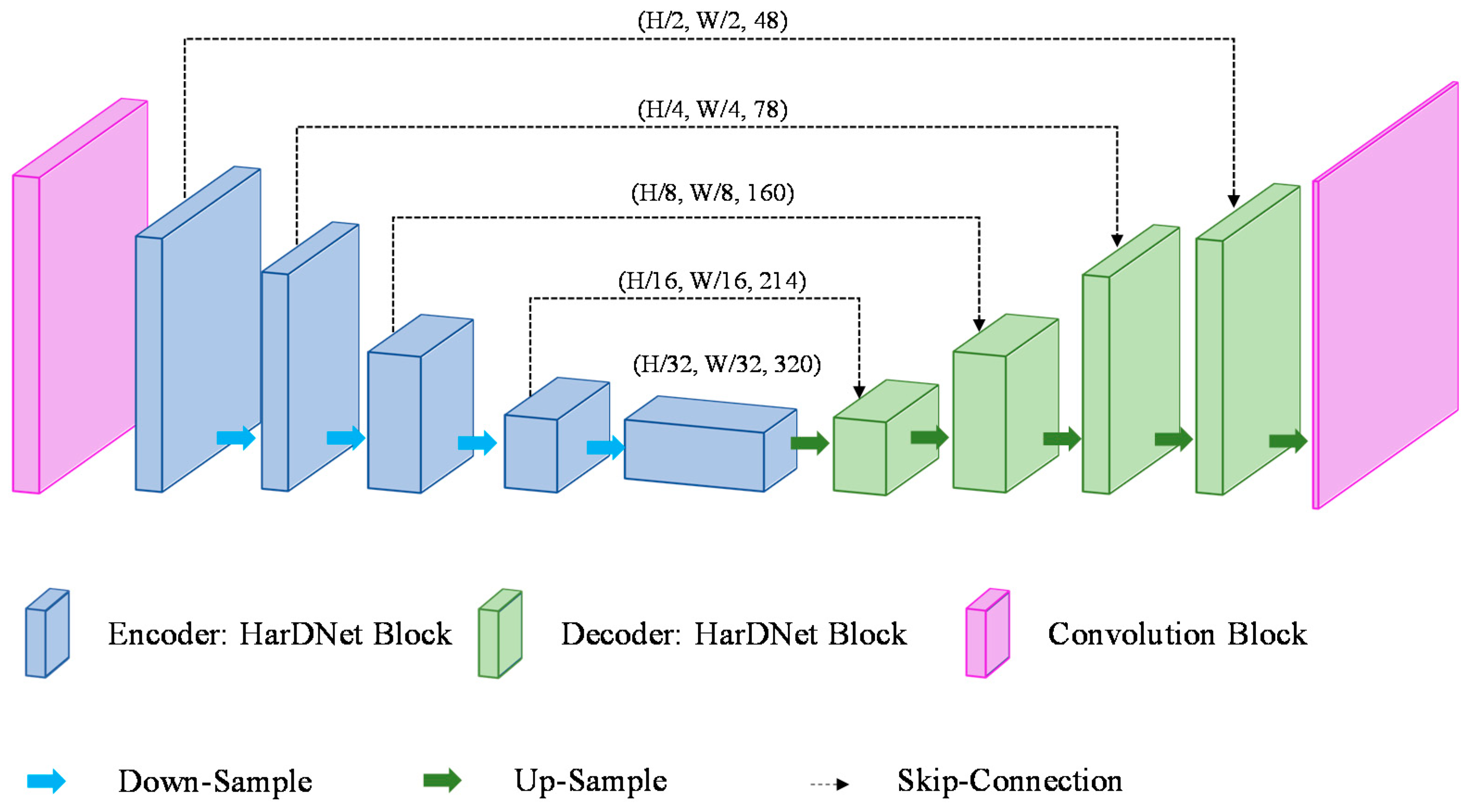
HarDNet is a model of U-Net form with an encoder–decoder structure built with the HarDNet block as a backbone. Figure 4 shows the structure of the HarDNet model. The encoder refers to a process of extracting a feature map while reducing the image size through the down-sampling process and the encoder consists of one convolution block, four HarDNet blocks, and four down-sampling blocks. The convolution block consists of a convolution layer where filter = 24, kernel size = 3, and stride = 2, and a convolution layer where filter = 48, kernel size = 3, and stride = 1. A down-sampling block consists of a convolution layer with kernel size = 1 and an AvgPoll2d layer with kernel size = 2 and stride = 2. The transition section (bottleneck) uses a HarDNet block to complete the parameter transfer of the encoder and the decoder. The decoder up-samples the feature map received from the bottleneck into the same size as the input and, at the same time, it finds the disease region in the feature map and displays it in the output image. The decoder outputs the final image of (W, H) size after going through four HarDNet blocks, five up-sampling blocks, and the last convolution layer with kernel size = 1. An up-sampling block consists of an interpolate function that uses the “bilinear” mode and a convolution layer with kernel size = 1.

Figure 4. Architecture of HarDNet.

If an input image is expressed in terms of (W (width), H (height), and C (channels)), the shape of the feature map calculated through the encoder’s convolution block is (W/2, H/2, 48). The feature map of (W/32, H/32, 286) is output through four HarDNet blocks and four down-sampling blocks. The decoder receives the feature map of (W/32, H/32, 320) output from the bottleneck as input and then outputs a feature map of (W, H, class) (the class refers to the number of disease categories in the data). Table 1 shows the HarDNet’s detailed structure and output examples, where the output size column shows examples where a grayscale image with a size of 224 × 224 is used as input.

Table 1. HarDNet’s structure and output examples.

Stage	Block Name	Details	Output Size
Input			224 × 224 × 1
Encoder	Conv Block	2 × Convolution	112 × 112 × 48
	HarDNet Block	4 × Convolution	112 × 112 × 48
	Down-sampling Block	1 × Convolution 1 × AvgPool2d	56 × 56 × 64
	HarDNet Block	4 × Convolution	56 × 56 × 78
	Down-sampling Block	1 × Convolution 1 × AvgPool2d	28 × 28 × 96
	HarDNet Block	8 × Convolution	28 × 28 × 160
	Down-sampling Block	1 × Convolution 1 × AvgPool2d	14 × 14 × 160
	HarDNet Block	8 × Convolution	14 × 14 × 214
	Down-sampling Block	1 × Convolution 1 × AvgPool2d	7 × 7 × 286
Bottle Neck	HarDNet Block	8 × Convolution	7 × 7 × 320
Decoder	Up-sampling Block	1 × Upsample 1 × Convolution	-
	HarDNet Block	8 × Convolution	14 × 14 × 214
	Up-sampling Block	1 × Upsample 1 × Convolution	-
	HarDNet Block	8 × Convolution	28 × 28 × 160
	Up-sampling Block	1 × Upsample 1 × Convolution	-
	HarDNet Block	4 × Convolution	56 × 56 × 78
	Up-sampling Block	1 × Upsample 1 × Convolution	-
	HarDNet Block	4 × Convolution	112 × 112 × 48
	Up-sampling Block	1 × Upsample 1 × Convolution	-
Output	Conv Block	1 × Convolution	224 × 224 × 2

4.2. Swin Transformer Block

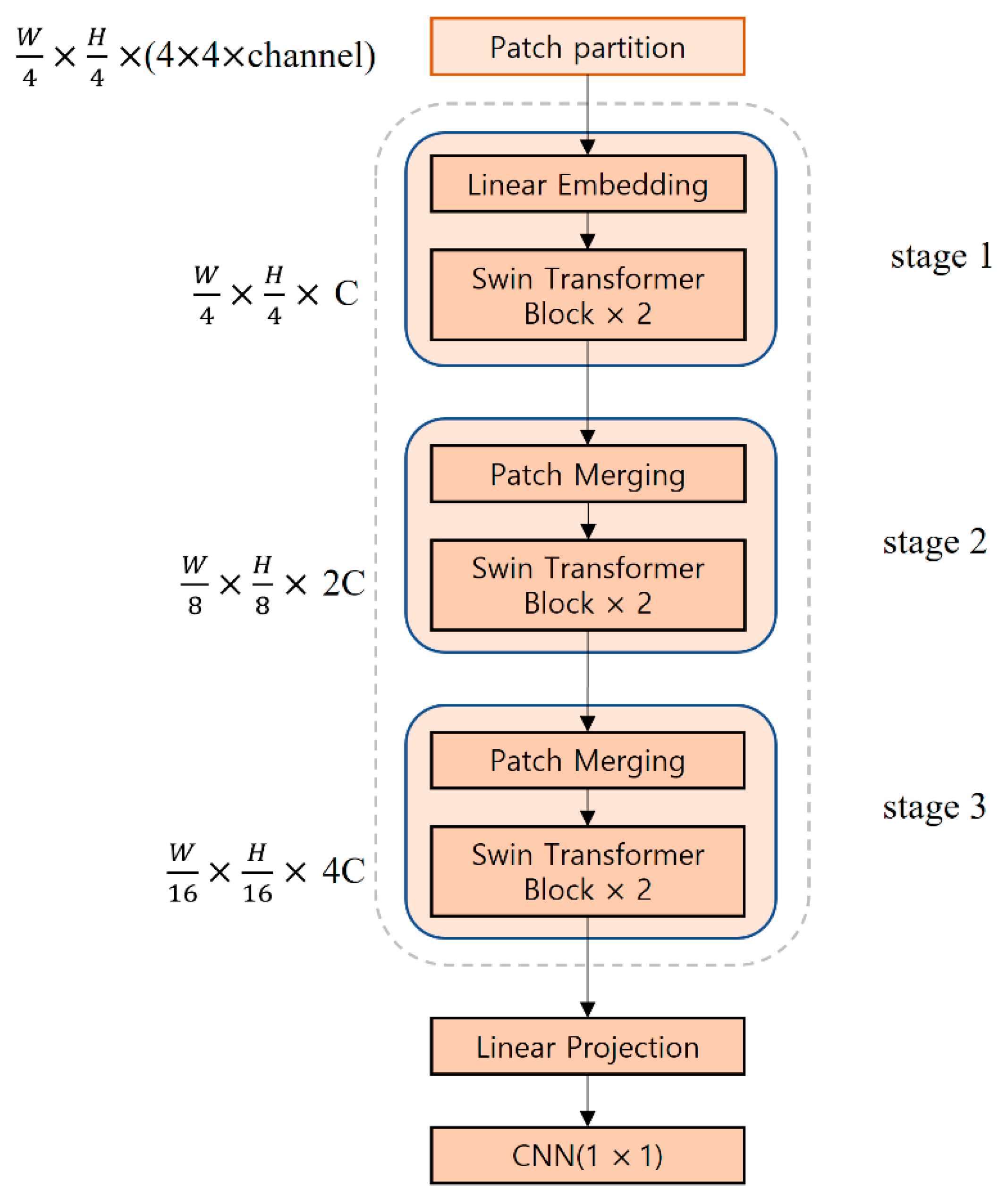
Figure 5 shows the structure of the Swin Transformer model used in this study. The input image passes through the patch partition layer and is segmented into patches with a 4 × 4 size to generate patch tokens having a shape of (W/4, H/4, 4 × 4 × channel). The generated patch tokens go through the linear embedding in stage 1. Afterward, they are input into two connected Swin transformer blocks to generate tokens of (W/4, H/4, C) where C refers to an arbitrary dimension. Stages 2 and 3 consist of patch merging and Swin transformer blocks, respectively. In patch merging, adjacent 2 × 2 patches are merged into one patch, and the tokens are down-sampled to 1/2, whereas C is doubled. In stages 2 and 3, the shape of the tokens is (W/8, H/8, 2C) and (W/16, H/16, 4C), respectively. In the Swin Transformer’s last “Linear Projection”, the feature dimension is expanded to eight times the input dimension, and after going through a 1 × 1 convolution, a feature map of the same shape is output. The Swin Transformer model receives a 112 × 112 × 48 feature map that was output from the first HarDNet block of the encoder, which is then connected to the last HarDNet block of the decoder. The window size of the Swin Transformer model used in this study is seven.

Figure 5. Architecture of the Swin Transformer.

4.3. STHArDNet: Combination of Swin Transformer with HarDNet

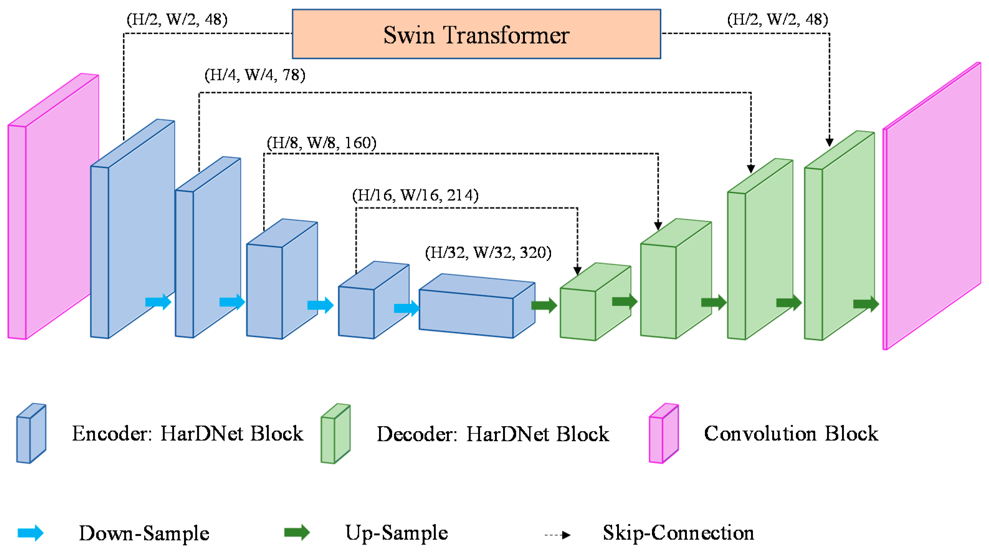
To combine the convolution with the vision transformer, this study proposes a STHarDNet model structure, as shown in Figure 6. STHarDNet consists of (1) the HarDNet with the encoder–decoder structure of the U-Net form and (2) the Swin Transformer used in skip connection that connects the encoder and the decoder.

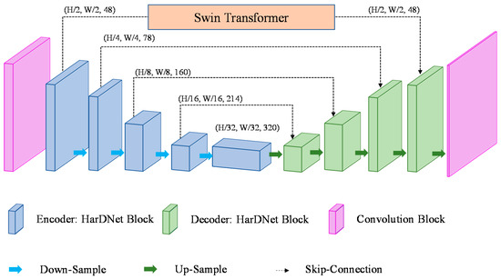
Figure 6. Architecture of the proposed STHarDNet model.

The Swin Transformer uses a hierarchical transformer to extract hierarchical feature maps and uses the shifted windows approach to calculate the relationship between patches in the whole feature map. Therefore, it has a more suitable model structure for segmentation than the transformer. However, the hierarchical transformer down-samples the feature map’s size by merging adjacent 2 × 2 patches to generate a hierarchical feature map. Therefore, if the input feature map’s size is small, the Swin Transformer cannot extract a deep hierarchical feature map.

Conventional combined models of CNN and transformer used the transformer in the bottleneck of the encoder and the decoder; however, the bottleneck has a small size (7 × 7) because its input is the feature map output at the end of the encoder. This is not suitable for the purpose of using the hierarchical transformer of the Swin Transformer in this study. Therefore, the Swin Transformer was not used at the bottleneck of the encoder and the decoder in this study, but used it in the first skip connection, where the size of the feature map was the largest among skip connections.

5. Experiments

5.1. Performance Evaluation Method

This study used four metrics—Dice, IoU (Intersection over Union, Jaccard index), precision, and recall—to evaluate the model’s performance. Dice is a metric used to measure the similarity between the predicted and actual values, and its value ranges from 0 to 1. The calculation equation is the same as that of F1-score, but there is a tendency to emphasize Dice more in the medical image segmentation field. Dice is also expressed as Dice coefficient, Dice similarity coefficient (DSC), and Dice score, depending on papers. IoU is a performance metric used in object detection and semantic segmentation studies and refers to the ratio of the intersection area to the union area for the predicted values and the actual values. IoU has the same meaning as Jaccard index. Precision refers to the percentage of the pixels predicted accurately in the prediction result of the model. Recall refers to how well the model detected the ground truths.

Dice, IoU, precision, and recall can all be calculated using True Positive (TP), True Negative (TN), False Positive (FP), and False Negative (FN) of the classification confusion matrix. Equations (6)–(9) show the calculation methods of the performance metrics, respectively.

$$Dice=\frac{2TP}{2TP+FP+FN}$$

(6)

$$IoU=\frac{TP}{TP+FP+FN}$$

(7)

$$Precision=\frac{TP}{TP+FP}$$

(8)

$$Recall=\frac{TP}{TP+FN}$$

(9)

As explained in Section 3, the ATLAS dataset has 3D MRI scan images, and the model’s performance was evaluated by measuring the performance at the patient level. In other words, instead of measuring the performance in the prediction result of one image, the disease of a patient was predicted using 189 MRI scan images captured for the patient as the input values of the model. In this study, the data of 52 patients were used as the validation data and obtained a total of 52 prediction results, which were then averaged

5.2. Experimental Setup and Parameter Settings

Table 2 shows the experimental setup used in this study. In the training process, the size of the input images in every model was set to 224 × 224 and the batch size was set to 16. Adam was used as an optimization function. The initial learning rate was set to 0.001, and if the validation loss did not decrease in five epoch cycles, the learning rate was decreased by 0.2 times. If the validation loss did not decrease in ten epoch cycles, early stopping was executed. As regards the loss function, the sum of the Dice loss and cross-entropy was used with the same weight.

Table 2. Experimental setup.

Device	Specifications
OS	Windows 10
CPU	Intel Core i9-9900KF 3.6GHz
GPU	NVIDIA GeForce RTX 2080Ti × 1
RAM	112GB
Storage	1TB SSD
Language	Python 3.7, PyTorch = 1.5

5.3. Performance Comparison Experiments

To validate the model proposed in this study, performance comparison experiments were conducted after selecting nine models that showed good performance in SOTA methods and the ATLAS dataset in past semantic segmentation studies. The SOTA models used in the experiments were typical U-Net-based models (U-Net, SegNet, PSPNet, and HarDNet) in the segmentation field with a CNN-based encoder–decoder structure; segmentation models (Swin Transformer and Swin UNet) using vision transformers; a model (TransHarDNet) that combined the CNN and vision transformer; and X-Net and D-UNet constructed to analyze the ATLAS data.

Table 3 shows the experimental results. The performances shown in Table 3 were obtained from the validation dataset after training the model with a separated dataset. In Table 3, the column “input type” refers to the input image shape of the model, “2D” refers to 2D grayscale images, and “3D” refers to 3D grayscale images. A 3D image was created by combining consecutive MRI scan images and the “output type” of every model was a 2D image. The 2D output corresponding to a 3D image input was based on the target value of the third image in the four consecutive MRI scan images that produced the 3D image and was the same as the 3D input/output used in D-UNet [2].

Table 3. Performance comparison of models in the ATLAS dataset.

Model Name	Input Type	Output Type	Dice	IoU	Precision	Recall
U-Net [4]	2D	2D	0.4517	0.3333	0.4831	0.5118
SegNet [23]	2D	2D	0.3751	0.2675	0.4418	0.3767
PSPNet [24]	2D	2D	0.4465	0.3282	0.5653	0.4200
HarDNet [14]	2D	2D	0.5066	0.3774	0.7358	0.4331
TransHarDNet	2D	2D	0.5051	0.3816	0.5785	0.5176
Swin Transformer [15]	2D	2D	0.1640	0.1053	0.7306	0.1247
Swin UNet [16]	2D	2D	0.4034	0.2883	0.5871	0.3402
X-Net [17]	2D	2D	0.4859	0.3670	0.6277	0.4391
D-UNet [18]	2D+3D	2D	0.4759	0.3570	0.4780	0.5248
STHarDNet	2D	2D	0.5170	0.3866	0.6222	0.4979
STHarDNet (Proposed)	3D	2D	0.5547	0.4184	0.6764	0.5286

As shown in Table 3, the STHarDNet proposed in this study resulted in a Dice of 0.517, IoU of 0.387, precision of 0.622, and recall of 0.498 when the “input type” and “output type” were both 2D. These performances were higher than those of existing SOTA models and stroke diagnostic models. Furthermore, when a 3D image was input and a 2D image was output, the proposed STHarDNet showed a Dice of 0.5547, IoU of 0.4184, precision of 0.6763, and recall of 0.5286, showing higher performances compared to when a 2D image was input. (The shape of the 3D input image of STHarDNet is 224 × 224 × 4).

The experimental results show that the Dice, IoU, precision, and recall performances of the HarDNet built based on a single CNN or a single Swin Transformer-based segmentation model were lower compared to those when the two models are all combined and used. This proves that, if the ViT-based Swin Transformer model and the CNN-based HarDNet model proposed in this study are combined, the performance can be improved compared to when a single model is used.

5.4. Speed Comparison Experiments of Models

The golden time for strokes from the onset to diagnosis and treatment was less than one hour. Therefore, not only the segmentation performance, but also the image process speed, are critically important for stroke diagnosis models. Therefore, comparative experiments of image processing speed were conducted with the STHarDNet and the models used in the performance comparison experiments. In the experiments, the time consumed and frames per second (FPS) were recorded when 100,000 images were processed, respectively, in the same environment. Table 4 shows the results of the experiments on the speed comparison of the models.

Table 4. Speed comparison of models.

Model Name	Input Image Size	100,000 Frames
		Seconds	FPS
U-Net	224 × 224	475.109	210.477
SegNet	224 × 224	415.869	240.459
PSPNet	224 × 224	637.318	156.907
HarDNet	224 × 224	325.117	307.58
TransHarDNet	256 × 256	352.066	284.036
Swin Transformer	224 × 224	1353.657	73.873
Swin UNet	224 × 224	414.798	241.081
X-Net	224 × 192	982.462	101.785
D-UNet	192 × 192	572.719	174.605
STHarDNet (Proposed)	224 × 224	333.395	299.943

In Table 4, HarDNet showed the fastest speed with 307.58 FPS when processing 100,000 images, whilst STHarDNet was the second fastest with FPS of 299.943 FPS. STHarDNet was 2.48% slower than HarDNet when performing calculations with 100,000 images, but the Dice and IoU performances were 9.49% and 10.89% better, respectively. Furthermore, when 100,000 images were calculated, the FPS was 42.5% faster than that of the U-Net, 71.78% faster than that of the D-UNet, and 5.6% faster than that of the TransHarDNet that used the transformer in the bottleneck of the HarDNet.

6. Conclusions

This study proposed a STHarDNet structure by combining the Swin Transformer and HarDNet and applied it to the segmentation of stroke MRI scan images. The STHarDNet consists of two models: an encoder–decoder model in a lightweight U-Net shape that consists of HarDNet blocks and a Swin Transformer model consisting of Swin transformer blocks that connect the encoder and the decoder in the first skip connection. STHarDNet has both the character of the CNN model that completes the task while simultaneously looking at the constraining parts, and the character of the transformer that completes the task while looking at the sequence data in all images. By applying the Swin Transformer to the first skip connection in the model, it can receive a feature map larger than the bottleneck as an input, thereby maintaining the advantage of hierarchical feature extraction and the shifted windows approach of the Swin Transformer.

To prove the superiority of the proposed model, the MRI scan images of 177 patients from the ATLAS dataset were used for training and the images of 52 patients were used for validation to conduct the performance comparison experiments with existing SOTA models in the segmentation field. When 224 × 224 × 1 grayscale images were used in the experiments, STHarDNet showed a Dice of 0.517, IoU of 0.387, precision of 0.622, and recall of 0.498, which was better than those of the existing SOTA models used in the experiment. Furthermore, when 224 × 224 × 4 3D images that gathered four consecutive grayscale images were entered as inputs, the proposed model showed a Dice of 0 0.5547, IoU of 0.4185, precision of 0.6764, and recall of 0.5286, showing higher performances compared to when 2D images were input. Moreover, when 100,000 images were processed in the comparative experiment of image processing speed with the existing SOTA models, the STHarDNet model achieved 299.943 FPS, which was 2.48% slower than HarDNet and the second fastest among the ten models. However, because the segmentation performance of STHarDNet was 9.49% higher in terms of the Dice and 10.89% higher in terms of IoU compared to that of HarDNet, it can be said that the proposed STHarDNet is the best when the performances and speed were both considered.

Through the experiments in this study, the excellent segmentation performance of STHarDNet that combined the Swin Transformer in the first skip connection of HarDNet was demonstrated. Furthermore, it was proven that, even if the transformer is connected to not only the bottleneck, but also the skip connection, the model’s performance could be enhanced while maintaining a fast calculation speed.

In this study, the model was developed based on 2D layers. The input 3D image was also analyzed with the 2D layers. In future research, we plan to modify the model with 3D layers to improve its performance.

References

- Badža, M.; Barjaktarović, M. Segmentation of Brain Tumors from MRI Images Using Convolutional Autoencoder. Appl. Sci. 2021, 11, 4317. [Google Scholar] [CrossRef]
- Ghosh, S.; Huo, M.; Shawkat, M.S.A.; McCalla, S. Using Convolutional Encoder Networks to Determine the Optimal Magnetic Resonance Image for the Automatic Segmentation of Multiple Sclerosis. Appl. Sci. 2021, 11, 8335. [Google Scholar] [CrossRef]
- Wu, S.; Wu, Y.; Chang, H.; Su, F.T.; Liao, H.; Tseng, W.; Liao, C.; Lai, F.; Hsu, F.; Xiao, F. Deep Learning-Based Segmentation of Various Brain Lesions for Radiosurgery. Appl. Sci. 2021, 11, 9180. [Google Scholar] [CrossRef]
- Ronneberger, O.; Fischer, P.; Brox, T. U-Net: Convolutional Networks for Biomedical Image Segmentation. In Proceedings of the International Conference on Medical Image Computing and Computer-Assisted Intervention, Munich, Germany, 5–9 October 2015; Springer: Cham, Switzerland, 18 November 2015; pp. 234–241. [Google Scholar]
- Wang, D.; Wu, Z.; Yu, H. TED-Net: Convolution-Free T2T Vision Transformer-Based Encoder-Decoder Dilation Network for Low-Dose CT Denoising. arXiv 2021, arXiv:2106.04650. [Google Scholar]
- Zhou, H.-Y.; Guo, J.; Zhang, Y.; Yu, L.; Wang, L.; Yu, Y. nnFormer: Interleaved Transformer for Volumetric Segmentation. arXiv 2021, arXiv:2109.03201. [Google Scholar]
- Carion, N.; Massa, F.; Synnaeve, G.; Usunier, N.; Kirillov, A.; Zagoruyko, S. End-to-End Object Detection with Trans-formers. In European Conference on Computer Vision; Springer: Cham, Switzerland, 2020; Volume 12346, pp. 213–229. [Google Scholar] [CrossRef]
- Zheng, S.; Lu, J.; Zhao, H.; Zhu, X.; Luo, Z.; Wang, Y.; Fu, Y.; Feng, J.; Xiang, T.; Torr, P.H.; et al. Rethinking Semantic Segmentation from a Sequence-to-Sequence Perspective with Transformers. In Proceedings of the 2021 IEEE/CVF Conference on Computer Vision and Pattern Recognition (CVPR), Nashville, TN, USA, 21–24 June 2021; pp. 6877–6886. [Google Scholar]
- Dosovitskiy, A.; Beyer, L.; Kolesnikov, A.; Weissenborn, D.; Zhai, X.; Unterthiner, T.; Dehghani, M.; Minderer, M.; Heigold, G.; Gelly, S.; et al. An Image Is Worth 16x16 Words: Transformers for Image Recognition at Scale. arXiv 2020, arXiv:2010.11929. [Google Scholar]
- Xu, G.; Wu, X.; Zhang, X.; He, X. LeViT-UNet: Make Faster Encoders with Transformer for Medical Image Segmentation. arXiv 2021, arXiv:2107.08623. [Google Scholar]
- Chang, Y.; Menghan, H.; Guangtao, Z.; Xiao-Ping, Z. TransClaw U-Net: Claw U-Net with Transformers for Medical Image Segmentation. arXiv 2021, arXiv:2107.05188. [Google Scholar]
- Chen, J.; Lu, Y.; Yu, Q.; Luo, X.; Adeli, E.; Wang, Y.; Lu, L.; Yuille, A.L.; Zhou, Y. TransUNet: Transformers Make Strong Encoders for Medical Image Segmentation. arXiv 2021, arXiv:2102.04306. [Google Scholar]
- Wang, W.; Chen, C.; Ding, M.; Yu, H.; Zha, S.; Li, J. TransBTS: Multimodal Brain Tumor Segmentation Using Transformer. In Lecture Notes in Computer Science; Springer: Cham, Switzerland, 2021; pp. 109–119. [Google Scholar] [CrossRef]
- Chao, P.; Kao, C.-Y.; Ruan, Y.; Huang, C.-H.; Lin, Y.-L. HarDNet: A Low Memory Traffic Network. In Proceedings of the 2019 IEEE/CVF International Conference on Computer Vision (ICCV), Seoul, Korea, 27 October–2 November 2019; pp. 3551–3560. [Google Scholar] [CrossRef] [Green Version]
- Liu, Z.; Lin, Y.; Cao, Y.; Hu, H.; Wei, Y.; Zhang, Z.; Lin, S.; Guo, B. Swin Transformer: Hierarchical Vision Transformer using Shifted Windows. arXiv 2021, arXiv:2103.14030. [Google Scholar]
- Cao, H.; Wang, Y.; Chen, J.; Jiang, D.; Zhang, X.; Tian, Q.; Wang, M. Swin-Unet: Unet-like Pure Transformer for Medical Image Segmentation. arXiv 2021, arXiv:2105.05537. [Google Scholar]
- Qi, K.; Yang, H.; Li, C.; Liu, Z.; Wang, M.; Liu, Q.; Wang, S. X-Net: Brain Stroke Lesion Segmentation Based on Depthwise Separable Convolution and Long-Range Dependencies. In Proceedings of the International Conference on Medical Image Computing and Computer-Assisted Intervention, Shenzhen, China, 13–17 October 2019; Springer: Cham, Switzerland, 2019; Volume 11766, pp. 247–255. [Google Scholar] [CrossRef] [Green Version]
- Zhou, Y.; Huang, W.; Dong, P.; Xia, Y.; Wang, S. D-UNet: A Dimension-Fusion U Shape Network for Chronic Stroke Lesion Segmentation. IEEE/ACM Trans. Comput. Biol. Bioinform. 2019, 18, 940–950. [Google Scholar] [CrossRef] [PubMed] [Green Version]
- Basak, H.; Hussain, R.; Rana, A. DFENet: A Novel Dimension Fusion Edge Guided Network for Brain MRI Segmentation. SN Comput. Sci. 2021, 2, 1–11. [Google Scholar] [CrossRef]
- Zhang, Y.; Wu, J.; Liu, Y.; Chen, Y.; Wu, E.X.; Tang, X. MI-UNet: Multi-Inputs UNet Incorporating Brain Parcellation for Stroke Lesion Segmentation From T1-Weighted Magnetic Resonance Images. IEEE J. Biomed. Health Inform. 2021, 25, 526–535. [Google Scholar] [CrossRef] [PubMed]
- Anatomical Tracings of Lesions after Stroke (ATLAS) R1.1. Available online: http://fcon_1000.projects.nitrc.org/indi/retro/atlas.html (accessed on 15 February 2021).
- Liew, S.-L.; Anglin, J.M.; Banks, N.W.; Sondag, M.; Ito, K.; Kim, H.; Chan, J.; Ito, J.; Jung, C.; Khoshab, N.; et al. A large, open source dataset of stroke anatomical brain images and manual lesion segmentations. Sci. Data 2018, 5, 180011. [Google Scholar] [CrossRef] [PubMed] [Green Version]
- Badrinarayanan, V.; Kendall, A.; Cipolla, R. SegNnet: A deep convolutional encoder-decoder architecture for image segmentation. IEEE Trans. Pattern Anal. Mach. Intell. 2017, 39, 2481–2495. [Google Scholar] [CrossRef] [PubMed]
- Zhao, H.; Shi, J.; Qi, X.; Wang, X.; Jia, J. Pyramid scene parsing network. In Proceedings of the 2017 IEEE Conference on Computer Vision and Pattern Recognition, Honolulu, HI, USA, 21–26 July 2017; pp. 2881–2890. [Google Scholar] [CrossRef] [Green Version]
Publisher’s Note: MDPI stays neutral with regard to jurisdictional claims in published maps and institutional affiliations. |
© 2022 by the authors. Licensee MDPI, Basel, Switzerland. This article is an open access article distributed under the terms and conditions of the Creative Commons Attribution (CC BY) license (https://creativecommons.org/licenses/by/4.0/).