Abstract
Cloud computing systems revolutionized the Internet, and web systems in particular. Quality of service is the basis of resource configuration management in the cloud. Load balancing mechanisms are implemented in order to reduce costs and increase the quality of service. The usage of those methods with adaptive intelligent algorithms can deliver the highest quality of service. In this article, the method of load distribution using neural networks to estimate service times is presented. The discussed and conducted research and experiments include many approaches, among others, application of a single artificial neuron, different structures of the neural networks, and different inputs for the networks. The results of the experiments let us choose a solution that enables effective load distribution in the cloud. The best solution is also compared with other intelligent approaches and distribution methods often used in production systems.
1. Introduction
The Internet is the primary medium that provides information; business services; telecommunication services; entertainment; and, during the COVID-19 pandemic, also other services, such as education and group meetings. To operate, internet services use servers based on web technologies.
In the past, companies providing web services built and maintained their own server rooms. Cooperating servers that formed web clusters were used to maintain more demanding services. Nowadays, more sophisticated approaches are used, namely, cloud computing. It is a new computing paradigm, according to which companies rent computer system resources on demand, without direct active management of it. Cloud computing systems enable access to a shared pool of resources such as servers, storage, and applications [1,2]. Organization of resources improves the performance, utilization of resources, and energy consumption management [3]. The popularity of the cloud attracts a variety of providers that offer a wide range of cloud-based services to users.
Cloud system belonging to one company is physically divided into regions (server rooms) placed in different geographical locations. The regions themselves are also divided into availability zones—physically separated parts of the regions with independent infrastructure and resources [4]. Availability zones contain different resources, including servers with efficient processors.
Quality of service (QoS) is the basis of cloud service and resource configuration management [5]. Load balancing mechanisms are implemented in order to reduce costs and increase quality of service. Such mechanisms are widely used in cluster-based systems. Effective distribution of load is still an open problem in cloud computing. New algorithms, methods, and architectures meeting clients’ demands still need to be developed.
In our previous work, we proposed many methods and solutions for load sharing and load distribution in cloud-based web systems [6,7,8,9]. Most of the solutions use a neuro-fuzzy approach to estimate the response time on different resources in the cloud. In this article, we present a new method of load distribution using artificial neurons and neural networks to estimate service times in the web system. The proposed method enables us to minimize the response time for every single HTTP request. While conducting the research, we tried many approaches including the application of a single artificial neuron, different structures of the neural networks, and different inputs for the networks. The experiments made it possible to choose an adequate solution for load distribution in the cloud. This enabled us to make a new design of load balancer designated for cluster-based web systems. The results obtained in the simulation experiments indicate that it is justified to continue the research in the environment of the real cloud computing system.
The rest of the article is composed as follows. In Section 2, the related work is presented with the motivation and problem to solve. Section 3 introduces a description of load balancer construction. In Section 4, the testbed is given. Section 5 contains a description of different neural networks used in the load balancer and the results obtained. Section 6 includes conclusions and directions for further research.
2. Related Work and Motivations
Cloud computing, like many other computing technologies, uses distributed systems in order to meet a very high demand for computing power. The load balancing methods [10] are used to distribute tasks and loads between nodes in the system. These methods help to improve resource utilization, shorten response times, and enable flexible scalability, which is an essential part of cloud computing [11,12].
The load balancing mechanisms used in internet clouds can be divided into three main categories [10,13,14,15,16]: static, dynamic, and adaptive. In static load balancing, tasks are performed with the usage of deterministic or probabilistic algorithms that do not take into account the current state of the system. Simple strategies have been popular since the beginning of cluster-based internet systems and they are still being refined. An example of such a strategy is Round Robin, which assigns incoming HTTP requests to successive servers. Xu Zongyu and Wang Xingxuan created a slightly more intelligent version that takes into account the load on the web server [17]. Stochastic strategies are also still being developed, and they are becoming more and more sophisticated [18,19,20].
In the dynamic approach, decisions are made on the basis of the current state of the system. The most popular dynamic load balancing algorithm in AWS (Amazon Web Services) [21] is Least Load, which assigns HTTP requests to nodes with the lowest value of the selected load measure.
The adaptive approach is the most complex. Decisions are made not only on the basis of the state of the system. As the environment changes, the operating strategy may also change. [22]. Most adaptation strategies use technics commonly called “intelligent approaches”. Many specialists claim that only this type of strategy can effectively ensure an acceptable access time to WWW content under the conditions of typical WWW traffic, characterized by self-similarity and burstiness [23,24,25,26]. Among many artificial intelligence techniques, the Ant Colony Optimization (ACO) algorithm [27], proposed by Kumar Nishant et al., can be distinguished. In the algorithm, the generated ants move along the width and length of the cloud network in such a way that they know the location of both underloaded and overloaded nodes. Another interesting method of distributing HTTP requests using strategies based on natural phenomena is the artificial bee colony (ABC) [25]. It uses a decision mechanism that mimics the behavior of a bee family. Another solution based on heuristic algorithms is the particle swarm optimization (PSO) strategy for scheduling requests to individual cloud components [28].
Artificial neural networks have also been used in adaptive load distribution systems [29,30,31]. A good example of an energy-sensitive solution is provided by Sallami et al. [32].
Over the past few years, there have been many publications on machine learning as applied to fair distribution of tasks in parallel and distributed systems. For example, Xu et al. [33] used reinforcement learning to maximize computational performance in distributed memory systems during particle motion simulation. Oikawa et al. [34] used machine learning for load balancing in distributed scientific computing. Chen et al. [35] used a multilayer perceptron perceptron to balance Linux workloads in accessing lower-level hardware resources. Load balancing in the cloud is also a subject of ongoing research—artificial neural networks including deep neural networks are often used in them [36,37]. The solution we present differs from the others in that the load balancing task has been decomposed into many parts—for each server and for each type of request. In each of these parts, the neural network does only one thing—it predicts the server’s response time.
Another group of intelligent adaptive approaches using fuzzy neural models was proposed by Zatwarnicki. These are solutions enabling global distribution between server rooms located in different geographic locations, e.g., GARD [38] and GARDIB [7], and also local approaches such as FARD [39] and FNRD [6] strategies. All systems presented in the solutions work in a way that minimizes the response time for each individual HTTP request. Our latest work [8,9,40,41] proposed a two-layer cloud architecture.
The results obtained showed significantly better performance for intelligent switches than for nonintelligent strategies.
Figure 1 shows a typical architecture of cluster-based web system with load balancer and many web servers. This architecture was used while conducting the research in this article.
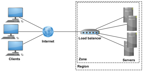
Figure 1.
Web cloud system diagram.
Taking into account the results of the latest research [40,41], we propose the design of a new load balancer that distributes the HTTP request among web servers placed in one location (one region) in this article. Furthermore, several solutions for request response time prediction using artificial neural networks were tested and applied in Load Balancer.
The detailed description of the proposed approach is presented in the subsequent sections.
3. Load Balancer
The primary purpose of an intelligent load balancer is to redirect incoming HTTP requests to web servers that are able to service requests in the shortest time. It can be expressed as in Equation (1):
where
—the chosen executor out of executors;
—an estimated response time to request for the -th server;
—the index of the request.
The load balancer (Figure 2) consists of the following modules: classification module (), measurement module (), decision module (), redirection module (), and executor models (), where . At first, an incoming HTTP request is assigned to the class and it is determined as to whether it is a static or dynamic () request in CM. The extracted information is transferred to modules.
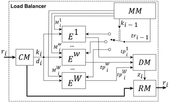
Figure 2.
The load balancer diagram.
The classification of requests is needed in order to better estimate the response time of incoming requests. Each request can have the status “dynamic” or “static” () depending on whether it refers to a script executed on the server (e.g., PHP, Python, Java) or whether a static file is downloaded (e.g., an image file). Additionally, the request is also assigned to one of the classes, depending on the type of an object requested and its size. Requests belonging to the same class have similar request response times. More detailed classification is presented in Section 5.5.
The measures the time of servicing requests on servers and their load, and then passes this information to modules.
The executor model estimates the response time of the corresponding server, taking into account its load where:
—the number of static requests processed on the at the time of arrival of the request ;
—the number of dynamic requests processed on the at the time of arrival of the request .
The executor models can adapt to the environment using previous response time .
The makes a decision according to Equation (1) using information from and modules. The module forwards the incoming request to the selected server.
4. Test Bed Used in the Experiments
In the further part of the article, various approaches to the construction and structure of the executor model are presented. In order to be able to assess the solutions adopted, we needed to develop a research environment, which is presented in this chapter.
Machine learning often uses a simulation environment at an earlier stage in the research (e.g., reinforcement learning). Creating such an environment involves preparing a policy and setting parameters that will imitate the real environment, and then adding an agent to the environment that will adapt to the given environment. For the initial training of an agent, establishing a policy to adapt to is more important than accurately reflecting the parameters of the real environment. An agent that can adapt well to the simulation environment will probably also be able to adapt to the real environment (although it has slightly different parameters). However, the measurements made show that the differences in the average response times obtained in the simulation and real environment do not exceed 20%, which according to the literature [42] is a sufficient value. After the initial selection of the algorithms used in the simulation environment, it is possible to proceed to the testing phase in a real distributed environment.
The simulation environment was created with the use of OMNeT ++ package. This system provides appropriate libraries and environment for simulation, and it is one of the most popular packages for evaluating network systems [43].
The simulation environment consisted of several modules that map the behavior of various elements of the real system, namely, HTTP request generator, load balancer, web servers, and database server. The simulator diagram is shown in Figure 3.
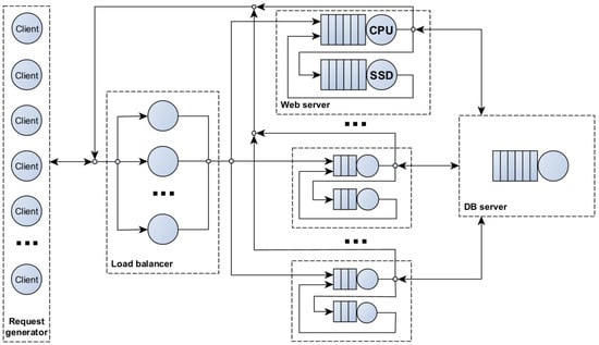
Figure 3.
The simulator diagram.
In order to determine the value of the real parameters of the elements of the simulation environment, we carried out preliminary experiments in a manner similar to that in [44]. The experiments were conducted on servers equipped with an Intel Core i7 7800X processor, a Samsung SSD 850 EVO driver, and 32 GB of RAM. The Apache server was running WordPress, the most commonly used CMS in the world, which is present on more than 25% of the world’s websites [45]. Thanks to this, it was possible to reproduce the behavior of many real business websites. Computers with higher performance are often used for servers, but only part of the resources (cores) is used for one virtual machine. The hardware whose parameters we used in the simulation usually do not differ in its performance from the average virtual machine used in general-purpose computing clouds, which are most often chosen for medium-sized business solutions.
The request generator module contained multiple clients, each simulating the behavior of a web browser. To download a website, we downloaded the content of the HTML file first, and then up to 6 TCP connections were opened to download the rest of the page, such as css, js, or images. The number of websites downloaded during one session was modeled using the inverse Gaussian distribution (μ = 3.86, λ = 9.46), according to human behavior. Regarding the time between the opening of subsequent pages (user think time), the Pareto distribution (α = 1.4, k = 1) was used [46]. Traffic in the network is generated synthetically on the basis of the observed behavior.
Each client simulated the download of a website whose parameters (type and size of HTML and nested objects) were the same as in the popular website https://www.sonymusic.com (accessed on 9 March 2019) [47] that also works through the WordPress CMS.
In the simulation environment, the web balancer was able to distribute HTTP requests with the usage of popular algorithms in Amazon AWS [21] and with the use of intelligent strategies, namely,
- Round Robin (RR);
- Least load (LL)—assigns HTTP requests to the servers with the lowest number of serviced HTTP requests (this strategy works very well in practical solutions and it is a kind of reference line);
- Fuzzy-neural request distribution (FNRD)—intelligent strategy using fuzzy-neural approach [6];
- Neural network (NN)—a new solution presented here, using neural networks.
The load balancer was modeled as a single queue in the simulation. Each of the web server modules contained separate CPU and SSD modeling queues. RAM acted as a cache for the file system. The database server has been modeled as a single queue. The response times for the above elements were obtained by measuring them on a real server with an Intel Xeon E5-2640 v3 processor.
The experiments were carried out for a cloud system with 20 WWW servers and 1 database server. The number of clients simulating different loads on the web system ranged from 100 to 2500.
In each experiment, 40 million HTTP requests were processed, the warming phase took about 10 million requests, and the response time for 30 million was measured.
5. Design of Executor Model
As it was previously described, the load balancer distributes HTTP requests to different web servers . There is one executor model associated with each server . The module estimates the time needed to respond to the request. On the basis of the results of the estimation for all servers, the server with the expected shortest response time is selected.
The description and research on the modules is given below.
Assuming that each of the requests can be serviced by one of the many servers , we found that it essential to choose the right one. Since each has one executor model associated with it, it is possible to specify different operating parameters for each server.
At the input to the executor, the parameters and are given, which characterize the incoming request. The executor input also includes information about the number of currently processed static requests and the number of processed dynamic requests on the server . The model also receives feedback on the real time of servicing the last request by the server (the index is arbitrary here since at the time of the next request, the previous one may not have been processed yet, and therefore its response time may also be unknown). The general diagram of the executor module is presented in Figure 4.
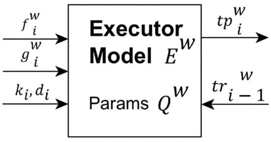
Figure 4.
The general diagram of the Executor Model .
The primary function of the executor model is to estimate the time . Since further considerations are made for a single executor model , there is no superscript in the markings and formulas.
The time is calculated as follows:
where
—function that depends on the current operation parameters at the time of the request
This module can operate in two modes, learning or prediction. Both modes take into account the current state of the server , the class of the incoming request , and the fact whether it is a dynamic request .
After servicing request by the server, the executor module learning step follows. The information needed in the prediction mode , and is also processed in this step. Additionally, the real response time of the last request on the server is taken into account. This allows the operating parameters to be modified in a way that enables predicted value to be closer to the real value.
The following subsections describe the various possible approaches to the executor model structure and parameterization. They also include the evaluation of these approaches.
Since requests are classified and requests belonging to the same class have a similar response time, a separate structure (), having different operating parameters , was extracted for each class, estimating the time. Each NM module contains an artificial neural network. Figure 5 presents the structure of the executor model. The inputs to the module are and , while decides which of the elements will be used in the estimation of the response time .
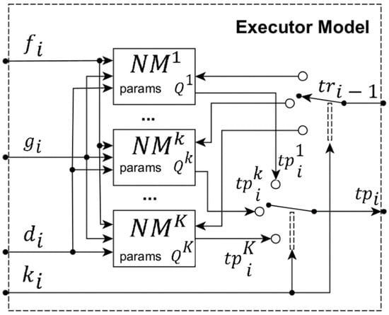
Figure 5.
Executor model diagram after taking into account the assumptions. —designed neural network module.
Load balancing is a relatively complex task, but in this article, it was decomposed into many components (for each server and for each type of request). In each of these parts, there is a single simple neural network that should do one thing—predict the response time depending on several parameters. Only the entire system, composed of many simple elements, is the server load balancing system. In the preliminary research for the article, the influence of various activation functions, the additional bias parameter, the narrowing of the range of possible weight values, the use of multilayer networks, and the use of information obtained from the neural network in the previous steps were investigated. Some of these activities did not improve the system operation. The article describes some of them, as well as the results obtained.
Neural networks with different structures and operating parameters will be used to implement the element. At the beginning, a single neuron with four inputs is used; then, it is expanded by adding a fifth input that will provide feedback from the last operation of the neural network. Finally, the application of multilayer networks is tested.
5.1. Single Neuron
At the beginning, the simplest element—a single neuron—is used as the element (Figure 6). Thus, we provide the following inputs of the neuron: , , , and . The output of the neuron is the value computed as the weighted sum of the inputs, where operating parameters are neuron weights.
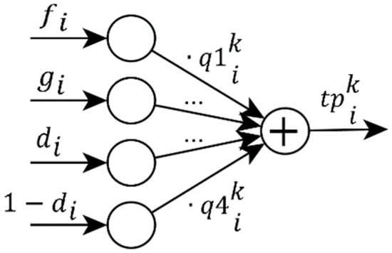
Figure 6.
Initial diagram of the executor model () element.
If the weights assume real values, it is possible to obtain an estimated time value as a negative value. Obviously, this is an error that can be corrected during model training, but it would have a negative impact on the speed at which satisfactory results are obtained. The research carried out shows that better results are obtained when only nonnegative weights are used in the learning process . The equation that describes this neural network is shown in Equation (3).
where
—takes the value 1 if the request is dynamic, and 0 if the request is static.
5.2. Model Training
For multilayer networks without recursion, the steepest gradient descent methods (most often the backpropagation method) are used for training. However, these methods often have a problem with falling into local minima and learning for a specific dataset, which reduces their usefulness when data from outside the set appear.
Model training consists in adjusting the parameters of all neural networks so that when the request arrives, the estimated time will be close to the real time needed for the server to service the request.
The method in which weights are randomly changed was adopted as the learning method. This method has the ability to break out of any local minimum and reach the global optimization minimum. In addition, this method does not have to be based only on one-way networks (recursions or any other connections are possible).
The method is as follows: each weight of the neural network is treated as a separate, independent variable, regardless of its place in the network. The weights are randomly modified with random values, but smaller changes are more likely (Gaussian distribution has been proposed). If the approximation error after the weight modification has decreased, then the new weights are adopted; otherwise, they are rejected. With some probability, the algorithm can generate any combination of changed weights, making it possible to leave the local minimum and search all available space.
The Box–Muller [48] transformation was used to generate values in the Gaussian distribution (4):
where:
i —independent samples chosen from the uniform distribution on the unit interval ;
i —independent random variables with a standard normal distribution and with standard deviation
5.3. Error Evaluation
When training the model, it is important to evaluate the error made by the module before and after modifying the parameters. The absolute percentage error () was taken as the measure of the error:
It is also possible to evaluate the mean absolute percentage error () of the model, taking into account the last requests (6):
However, evaluating the for too high may result in excessive computation time that should be performed in real time (without causing significant system delays). Too high n may also cause the system to become unreliable and unable to respond quickly enough to changes taking place in the server and in the characteristics of incoming requests.
5.4. Determining Optimal Parameters for Adaptation
Due to the Gaussian distribution, any change of the weight values is possible. However, the selection of the appropriate standard deviation (sd) may improve the results of the neural network adaptation.
To select the best standard deviation value, we performed experiments for subsequent values of this parameter (). For each value, the average response times of requests in the system were examined. The changes in the request handling times were not too large. Therefore, the diagram (Figure 7) narrowed the view only to measurements for high system load. Another modification of the algorithm was concerned with the fact that for each request, during learning, several attempts are made to change the weights with different values of standard deviations (). The last method (tentatively named ) turned out to be slightly more effective for the highest workloads of the system. This method was used in subsequent studies.
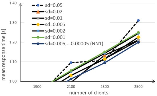
Figure 7.
Charts of the average request service time for different values of the standard deviation used for the modification of weights.
5.5. Request Class Analysis
The next study was concerned with the influence of the division of requests into classes. The division into classes can also affect the time needed to response the requests. Requests differ from each other depending on what objects are expected, and it is especially important whether it is a dynamic object (script executed on the server) or a static object (downloaded file). The size of the requested files is also significant. The average time to handle such a script or to download a file of a certain size is crucial in the classification of the resource. Some objects may have similar response times. Therefore, the combination of request types into smaller or larger groups was considered, hereinafter referred to as request classes. Then, a separate neural network was built for each of these request classes.
In the beginning, preliminary tests were performed. The tests were conducted for a very low load on the servers (small number of clients). Only requests made without waiting in the queue on the server were taken into account for the statistics. For each type of request, the number of requests during the simulation and their total execution time were counted. On this basis, we also calculated the average request execution time for each type. Then, the request types were sorted according to average execution time. The next step was to create request classes by combining these request types with similar average response times.
The first method of division into classes was used so that the number of requests for these classes was balanced. This means that, during simulation, some types of requests were more frequent, and some less frequent. If for a certain class of requests, only a few requests were generated during the simulation, it was not enough for the neural network serving this request to learn correctly. Therefore, the grouping of requests into classes was aimed at ensuring that each network had a similar amount of data that needed to be processed. The division was made into 1, 5, 10, 20, 35, 70, and 140 groups. The simulation results for each division are presented in Figure 8.
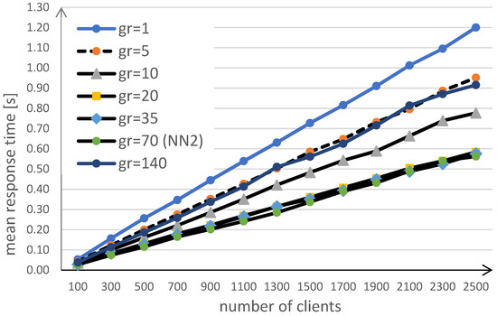
Figure 8.
Division into groups with a balanced number of requests.
The lowest value of the average response time for the load of 2500 clients was obtained for the division into 70 groups (tentatively named ), which was 0.56 s.
In another split method, it was assumed that requests in each group are served in a similar total time. This means that classes that serve “small” requests process more requests, while classes with higher average request response times process fewer requests. The results of such a division are shown in Figure 9.
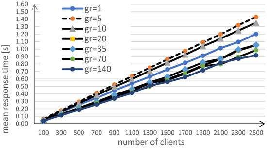
Figure 9.
The division into groups with a balanced total time of requests processing.
The lowest value of the average response time for the load of 2500 clients was obtained for the division into 140 groups, and it was as much as 0.92 s.
The division into 70 groups, in such a way that balances the number of requests for each group, turned out to be the most advantageous (marked as in the chart in Figure 8). This method of division was adopted for further research.
5.6. Additional Input
Then, we proposed adding a fifth input, which would implement a state memory of the module . An additional input was used for each neural network in several variants (Equations (7)–(9)):
- (1)
- the last predicted request () response time was given to the input;
- (2)
- the last request response time () was given to the input;
- (3)
- the difference between the response time () of the last request and its estimated value () was given to the input.
The diagrams of proposed neural networks are shown in Figure 10, while the simulation results are presented in Figure 11.
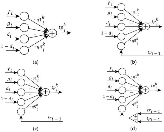
Figure 10.
Diagrams of modified neural networks: (a) before modification—four inputs; (b) on the fifth input—the estimated time of the last request; (c) on the fifth input—the time of the last request; (d) on the fifth input—the difference between the response time of the last request and its estimated value.
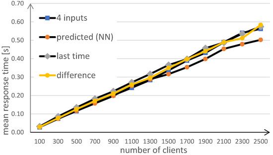
Figure 11.
Comparison of the results for modified neural networks.
The lowest value of the average response time for the load of 2500 clients was obtained for the fifth input with the last estimated request response time, and it was 0.50 s (marked as in the chart). This structure of neural networks was used for further research.
5.7. Multilayer Networks
The structure of neural networks tested thus far was the basic structure (one neuron, no hidden layers). The next step in the research was to expand the network by one or two hidden layers. The complexity of the neural network should be adapted to the complexity of the problem to be solved. Too simple and too complex structures will yield worse results. The structures of the networks studied are shown in Figure 12.
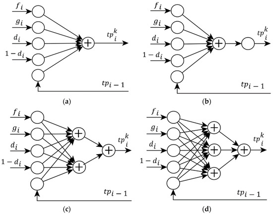
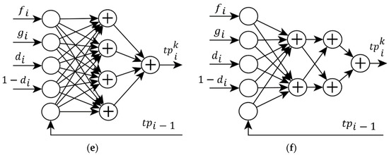
Figure 12.
Diagrams of modified neural networks: (a) before modification—1 neuron, no hidden layers; (b) 1 hidden layer containing 1 neuron; (c) 1 hidden layer containing 2 neurons; (d) 1 hidden layer containing 3 neurons; (e) 1 hidden layer containing 4 neurons; (f) 2 hidden layers, each with 2 neurons.
Each of the tested networks had five inputs in the same configuration as the best solution from the previous study . The inputs are as follows:
- the number of static tasks currently serviced on the server;
- the number of dynamic tasks currently serviced on the server;
- is the current task dynamic (value 1—dynamic task, 0—static);
- is the current task static (value 1—static task, 0—dynamic);
- value of the last predicted request response time.
The networks differed in the presence of neurons in hidden layers. The version without hidden layers (earlier solution), 1, 2, 3, and 4 neurons in one hidden layer (Figure 9) and two neurons in two hidden layers (Figure 9) were used. Networks have a linear activation function.
The results obtained from the experiments conducted for neural networks are presented in Figure 13. The chart shows that the best results for this task were obtained by neural networks with a simple structure (marked as NN in the graph), without hidden layers.
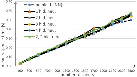
Figure 13.
Comparison of the results for modified neural networks.
5.8. Comparison with Other Algorithms
The results obtained were compared with the results in the following experiment steps ( and ) and with other popular load balancing algorithms— (fuzzy-neural request distribution), (request handling by the server loaded with the least number of requests), and (request handling in circular order). The results of the comparison of mean response time are shown in Figure 14. Table 1 presents the data in tabular form.
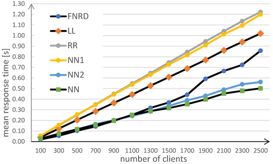
Figure 14.
Results of the comparison of mean response time. Compared algorithms: the proposed algorithm (NN) with the following research steps (NN1, NN2) and other popular methods of web server load balancing—FNRD, LL, RR.

Table 1.
Results of the comparison of mean response time in tabular form.
Another metric by which the algorithms can be compared is the 95 percentile of response time. The results of the comparison of 95 percentile of response time are shown in Figure 15. Table 2 presents the data in tabular form.
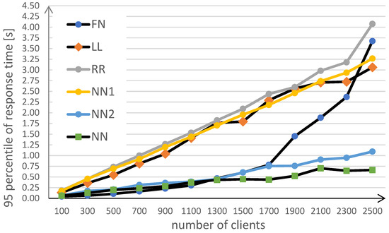
Figure 15.
Results of the comparison of 95 percentile of response time. Compared algorithms: the proposed algorithm (NN) with the following research steps (NN1, NN2) and other popular methods of web server load balancing—FNRD, LL, RR.

Table 2.
Results of the comparison of 95 percentile of response time in tabular form.
The results presented show that the proposed method provides shorter response time results compared to other popular methods and it is also stable for high loads.
5.9. Conclusions and Further Research
The developed method consists in the decomposition of a relatively complex task, which is load balancing in web servers, into many small tasks. For each of these subtasks, a neural network is designated that estimates the response time to requests. The best results were obtained when separate elements predicting times for different servers and request categories were made (i.e., one neural network provides only service times for one server and one type of request). Both the types of requests and the load on the servers change in the simulated environment. Each neural network specializes in a small portion of the tasks reaching the load balancer—this helps it adapt more accurately.
In future studies, the authors intend to perform tests in a real distributed environment. An additional research direction will be an attempt to use neural networks that will adapt not only by changing weights but also by changing the structure of connections.
6. Summary
Quality of service includes many aspects such as customer satisfaction and cost reduction. The authors of this article focused on one of them, i.e., the request response time. In this article, we presented a decision-making algorithm and method applied in load balancer working in the cluster-based web system. The decision mechanism uses the neural approach to predict response times of processing HTTP requests in web servers. Several different configurations were tested. Among others, we used single-neuron and multilayer networks, different inputs, and parameters affecting the adaptation process.
A simulation environment was designed and implemented to evaluate the proposed method. The simulator correctly imitated the behavior of web clients, as well as the operation of the web switch, web servers, and database. For all workloads, the proposed distribution method outperformed the non-intelligent strategies in the simulation environment. For high server loads, the neural approach also achieved shorter times than the other intelligent strategies.
It should be noted that all tests were carried out with the use of a simulator. Another goal of the authors is to obtain research results in a real distributed environment. The results of the research indicate that the presented new solution introduces an improvement in the simulated environment, and it is worth conducting further research on neural decision-making systems.
Author Contributions
Funding
This research received no external funding.
Institutional Review Board Statement
Not applicable.
Informed Consent Statement
Not applicable.
Conflicts of Interest
The authors declare no conflict of interest.
References
- Lee, B.T.G.; Patt, R.; JeffVoas, C. DRAFT Cloud Computing Synopsis and Recommendations. 2011. Available online: http://csrc.nist.gov/publications/nistpubs/800-146/sp800-146.pdf (accessed on 9 January 2020).
- Puthal, D.; Sahoo, B.; Mishra, S.; Swain, S. Cloud computing features, issues, and challenges: A big picture. In Proceedings of the 2015 International Conference on Computational Intelligence and Networks, Odisha, India, 12–13 January 2015; IEEE: Manhattan, NY, USA, 2015; pp. 116–123. [Google Scholar]
- Montes, J.; Sánchez, A.; Memishi, B.; Pérez, M.S.; Antoniu, G. GMonE: A complete approach to cloud monitoring. Future Gener. Comput. Syst. 2013, 29, 2026–2040. [Google Scholar] [CrossRef] [Green Version]
- Montes, J.; Sánchez, A.; Pérez, M.S. Riding out the storm: How to deal with the complexity of grid and cloud management. J. Grid Comput. 2012, 10, 349–366. [Google Scholar] [CrossRef] [Green Version]
- Zhang, L.; Zhang, Y.; Jamshidi, P.; Xu, L.; Pahl, C. Service workload patterns for Qos-driven cloud resource management. J. Cloud Comput. 2015, 4, 281. [Google Scholar] [CrossRef] [Green Version]
- Zatwarnicki, K. Adaptive control of cluster-based Web systems using neuro-fuzzy models. Int. J. Appl. Math. Comput. Sci. 2012, 22, 365–377. [Google Scholar] [CrossRef] [Green Version]
- Zatwarnicki, K. Guaranteeing quality of service in globally distributed web system with brokers. In Lecture Notes in Computer Science; Springer: Singapore, 2011; Volume 6923, pp. 374–384. [Google Scholar]
- Zatwarnicki, K.; Zatwarnicka, A. Cooperation of neuro-fuzzy and standard cloud web brokers. In Information Systems Architecture and Technology: Proceedings of 40th Anniversary International Conference on Information Systems Architecture and Technology—ISAT 2019; Borzemski, L., Świątek, J., Wilimowska, Z., Eds.; Springer: Cham, Switzerland, 2019; pp. 243–254. [Google Scholar]
- Zatwarnicki, K.; Zatwarnicka, A. A Comparison of request distribution strategies used in one and two layer architectures of web cloud systems. In Computer Networks; Springer: Singapore, 2019; Volume 1039, pp. 178–190. [Google Scholar]
- Alakeel, A. A guide to dynamic load balancing in distributed computer systems. Int. J. Comput. Sci. Inf. Secur. 2010, 10, 153–160. [Google Scholar]
- Rimal, B.P. Architectural requirements for cloud computing systems: An enterprise cloud approach. J. Grid Comput. 2011, 9, 3–26. [Google Scholar] [CrossRef]
- Ponce, L.M.; Dos Santos, W.; Meira, W.; Guedes, D.; Lezzi, D.; Badia, R.M. Upgrading a high performance computing environment for massive data processing. J. Internet Serv. Appl. 2019, 10, 19. [Google Scholar] [CrossRef] [Green Version]
- Nuaimi, K.A. A Survey of Load Balancing in Cloud Computing: Challenges and Algorithms. In Proceedings of the 2012 Second Symposium on Network Cloud Computing and Applications, London, UK, 3–4 December 2012; IEEE: Manhattan, NY, USA, 2012. [Google Scholar]
- Zenon, C.; Venkatesh, M.; Shahrzad, A. Availability and load balancing in cloud computing. In Proceedings of the International Conference on Computer and Soft modeling IPCSI, Singapore, 23 February 2011. [Google Scholar]
- Campêlo, R.A.; Casanova, M.A.; Guedes, D.O.; Laender, A.H.F. A brief survey on replica consistency in cloud environments. J. Internet Serv. Appl. 2020, 11, 1. [Google Scholar] [CrossRef]
- Afzal, S.; Kavitha, G. Load balancing in cloud computing—A hierarchical taxonomical classification. J. Cloud Comput. 2019, 8, 22. [Google Scholar] [CrossRef] [Green Version]
- Xu, Z.; Xingxuan, W. A predictive modified round robin scheduling algorithm for web server clusters. In Proceedings of the 34th Chinese Control Conference, Hangzhou, China, 28–30 July 2015; IEEE: Manhattan, NY, USA, 2015. [Google Scholar]
- Patiniotakis, I.; Verginadis, Y.; Mentzas, G. PuLSaR: Preference-based cloud service selection for cloud service brokers. J. Internet Serv. Appl. 2015, 6, 26. [Google Scholar] [CrossRef] [Green Version]
- Brototi, M.; Dasgupta, K.; Dutta, P. Load balancing in cloud computing using stochastic hill climbing-a soft computing ap-proach. In Proceedings of the 2nd International Conference on Computer, Communication. Control and Information Technology (C3IT), Coimbatore, India, 26–28 October 2012. [Google Scholar]
- Walczak, M.; Marszalek, W.; Sadecki, J. Using the 0–1 test for chaos in nonlinear continuous systems with two varying parameters: Parallel computations. IEEE Access 2019, 7, 154375–154385. [Google Scholar] [CrossRef]
- Amazon. How Elastic Load Balancing Works. 2019. Available online: https://docs.aws.amazon.com/elasticloadbalancing/latest/userguide/how-elastic-load-balancing-works.html (accessed on 23 January 2020).
- Rafique, A.; Van Landuyt, D.; Truyen, E.; Reniers, V.; Joosen, W. SCOPE: Self-adaptive and policy-based data management middleware for federated clouds. J. Internet Serv. Appl. 2019, 10, 2. [Google Scholar] [CrossRef] [Green Version]
- Crovella, M.; Bestavros, A. Self-similarity in World Wide Web traffic: Evidence and possible causes. IEEE/ACM Trans. Netw. 1997, 5, 835–846. [Google Scholar] [CrossRef] [Green Version]
- Domanska, J.; Domanski, A.; Czachorski, T. The influence of traffic self-similarity on QoS mechanisms. In Proceedings of the 2005 Symposium on Applications and the Internet Workshops (SAINT 2005 Workshops), Trento, Italy, 31 January–4 February 2005. [Google Scholar]
- Remesh Babu, K.R.; Samuel, P. Enhanced bee colony algorithm for efficient load balancing and scheduling in cloud. In Innovations in Bio-Inspired Computing and Applications; Springer: Cham, Switzerland, 2016; Volume 424, pp. 67–78. [Google Scholar]
- Suchacka, G.; Dembczak, A. Verification of web traffic burstiness and self-similarity for multiple online stores. Adv. Intell. Syst. Comput. 2017, 655, 305–314. [Google Scholar]
- Nishant, K.; Sharma, P.; Krishna, V.; Gupta, C.; Singh, K.P.; Nitin; Rastogi, R. Load balancing of nodes in cloud using ant colony optimization. In Proceedings of the 2012 UKSim 14th International Conference on Computer Modelling and Simulation, Cambridge, UK, 28–30 March 2012; IEEE: Manhattan, NY, USA, 2012. [Google Scholar]
- Suraj, P.; Wu, L.; Mayura, S.; Guru, S.M.; Buyya, R. A particle swarm optimization-based heuristic for scheduling workflow ap-plications in cloud computing environments. In Proceedings of the 24th IEEE International Conference on Advanced Information Networking and Applications, Perth, WA, Australia, 20–23 April 2010. [Google Scholar]
- Sharifian, S.; Akbari, M.K.; Motamedi, S.A. An Intelligence Layer-7 Switch for Web Server Clusters. In Proceedings of the 3rd International Conference: Sciences of Electronic, Technologies of Information and Telecommunications, Sousse, Tunisia, 27–31 March 2005; pp. 8–24. [Google Scholar]
- Boutaba, R.; Salahuddin, M.A.; Limam, N.; Ayoubi, S.; Shahriar, N.; Estrada-Solano, F.; Caicedo, O.M. A comprehensive survey on machine learning for networking: Evolution, applications and research opportunities. J. Internet Serv. Appl. 2018, 9, 16. [Google Scholar] [CrossRef] [Green Version]
- Lee, S.P.; Nahm, E.S. Development of an optimal load balancing algorithm based on ANFIS modeling for the clustering web-server. Commun. Comput. Inf. Sci. 2012, 310, 783–790. [Google Scholar]
- Sallami NM, A.; Daoud, A.A.; Alousi, S.A. Load balancing with neural network. Int. J. Adv. Comput. Sci. Appl. 2013, 4, 138–145. [Google Scholar]
- Xu, J.; Guo, H.; Shen, H.; Raj, M.; Wurster, S.W.; Peterka, T. Reinforcement Learning for Load-balanced Parallel Particle Tracing. arXiv 2021, arXiv:abs/2109.05679. [Google Scholar]
- Oikawa, A.; Freitas, V.; Castro, M.; Pilla, L. Adaptive load balancing based on machine learning for iterative parallel ap-plications. In Proceedings of the 28th Euromicro International Conference on Parallel, Distributed and Network-Based Processing (PDP), Västerås, Sweden, 11–13 March 2020. [Google Scholar]
- Chen, J.; Banerjee, S.S.; Kalbarczyk, Z.T.; Iyer, R.K. Machine learning for load balancing in the Linux kernel. In Proceedings of the Proceedings of the 11th ACM SIGOPS Asia-Pacific Workshop on Systems, Tsukuba, Japan, 24–25 August 2020; Association for Computing Machinery: New York, NY, USA, 2020; pp. 67–74. [Google Scholar] [CrossRef]
- Agarwal, R.; Sharma, D.K. Machine learning & Deep learning based Load Balancing Algorithms techniques in Cloud Computing. In Proceedings of the 2021 International Conference on Innovative Practices in Technology and Management (ICIPTM), Noida, India, 17–19 February 2021; pp. 249–254. [Google Scholar] [CrossRef]
- Pourkiani, M.; Abedi, M. Using Machine Learning for Task Distribution in Fog-Cloud Scenarios: A Deep Performance Analysis. In Proceedings of the 2021 International Conference on Information Networking (ICOIN), Jeju Island, Korea, 13–16 January 2021; pp. 445–450. [Google Scholar] [CrossRef]
- Borzemski, L.; Zatwarnicki, K.; Zatwarnicka, A. Adaptive and intelligent request distribution for content delivery networks. Cybern. Syst. 2007, 38, 837–857. [Google Scholar] [CrossRef]
- Borzemski, L.; Zatwarnicki, K. A fuzzy adaptive request distribution algorithm for cluster-based Web systems. In Proceedings of the 11th Euromicro Conference on Parallel Distributed and Network Based Processing, Genova, Italy, 5–7 February 2003; IEEE Press: Manhattan, NY, USA, 2003. [Google Scholar]
- Zatwarnicki, K. Two-level fuzzy-neural load distribution strategy in cloud-based web system. J. Cloud Comput. 2020, 9, 30. [Google Scholar] [CrossRef]
- Zatwarnicki, K. Providing predictable quality of service in a cloud-based web system. Appl. Sci. 2021, 11, 2896. [Google Scholar] [CrossRef]
- Menascé, D.; Almeida, V. Capacity Planning for Web Services; Prentice Hall: Upper Saddle River, NJ, USA, 2002. [Google Scholar]
- OMNeT++ Discrete Event Simulator. 2020. Available online: https://www.omnetpp.org/ (accessed on 2 February 2020).
- Zatwarnicki, K. Determination of parameters of parameters of web server simulation model. In Information Systems Architecture and Technology: Web Information Systems, Models, Concepts & Challenges; Springer: Cham, Switzerland, 2008; pp. 25–36. [Google Scholar]
- Munford, M. How WordPress Ate the Internet in 2016. And the World in 2017. Available online: https://www.forbes.com/sites/montymunford/2016/12/22/how-wordpress-ate-the-internet-in-2016-and-the-world-in-2017/ (accessed on 2 January 2020).
- Cao, J.; Cleveland, S.W.; Gao, Y.; Jeffay KSmith, F.D.; Weigle, M.C. Stochastic models for generating synthetic HTTP source traffic. In Proceedings of the Twenty-Third Annual Joint Conference of the IEEE Computer and Communications Societies, Hong Kong, 7–11 March 2004; pp. 1547–1558. [Google Scholar]
- Sony Music. Main Page. 2019. Available online: https://www.sonymusic.com/ (accessed on 9 March 2019).
- Box, G.E.P.; Muller, M.E. A Note on the Generation of Random Normal Deviates. Ann. Math. Stat. 1958, 29, 610–611. [Google Scholar] [CrossRef]
Publisher’s Note: MDPI stays neutral with regard to jurisdictional claims in published maps and institutional affiliations. |
© 2021 by the authors. Licensee MDPI, Basel, Switzerland. This article is an open access article distributed under the terms and conditions of the Creative Commons Attribution (CC BY) license (https://creativecommons.org/licenses/by/4.0/).