Abstract
Simulation models are elements of science that use software tools to solve complex mathematical problems. They are beneficial in areas such as performance engineering and communications systems. Nevertheless, to achieve more accurate results, researchers should use more detailed models. Having an analysis of the system operations in the early modeling phases could help one make better decisions relating to the solution. In this paper, we introduce the use of the QPME tool, based on queueing Petri nets, to model the system stream generator. This formalism was not considered during the first tool development. As a result of the analysis, an alternative design model is proposed. By comparing the behavior of the proposed generator against the one already developed, a better adjustment of the stream to the customer’s needs was obtained. The study results show that appropriately adjusting queueing Petri net models can help produce better streams of data (tokens).
1. Related Work
Performance evaluation is applied in communications system development and assessment. In recent years, most of the works focused on systems that were very efficient, and able to handle numerous incoming requests. The topic of stream preparation was omitted.
Authors model systems in different ways [1,2]. On the one hand, there are formal models used to analyze performance [3,4]. On the other hand, to describe systems, they use simulation models: QNs [5,6], CPN [5,7] or QPN [8,9,10]. In recent years, most works focused on web systems [4,6,11,12], which are very efficient, and able to handle numerous incoming requests. Moreover, QPNs are useful models in regard to specifying and verifying, e.g., protocol behaviors [13].
Usually some kind of workload generator is applied to analyze the behavior of the modeled system. A survey of such generators for general purpose web-based systems is presented in [14]. Specialized traffic models may be considered for different systems, e.g., for industrial networks [15] or streaming video data, both for input [16] and output streams [17]. In such models, an input stream generator is usually a part of the workload generator. Such an arrival stream generator produces a stream of random input data according to the expected distribution. Petri net models of the system typically are built based on predefined structures–patterns [18,19]; in such an approach, a stream generator is one of the integral components.
We created a stream generator (SG) client model using queueing Petri nets (QPNs), which guarantee performance analysis [12]. QPNs provide greater modeling power than queueing net (QN) and Petri net (PN) models. We used two types of formal models that were exploited in one model. Queueing Petri nets have the advantages of queueing nets (e.g., the network efficiency and evaluation of the system performance) and Petri nets (e.g., logical assessment of the system correctness). To the best of our knowledge, none of the existing techniques presented in the literature enable the preparation of such a stream. Falko Bause et al. in [20] describe these kinds of Petri nets, named QPNs. Kounev et al. [21] provide an introduction to QPNs.
The modeling approach presented in this paper differs from that of previous works [9], in regard to performance analysis, because we modeled different stream behaviors; they are similar to [7], but we prepared the SG based on another formalism. This approach could be treated as an extension of the paper [7].
In [7], colored Petri nets (CPNs) were used to model the SG. Two different ways were considered to impose restrictions on mapping between users and resources—transition guards or arc expressions. In this paper, QPNs are used instead of CPNs. Appropriate mapping in the output stream was achieved by means of transition modes and firing weights.
2. QPN Model
2.1. QPNs
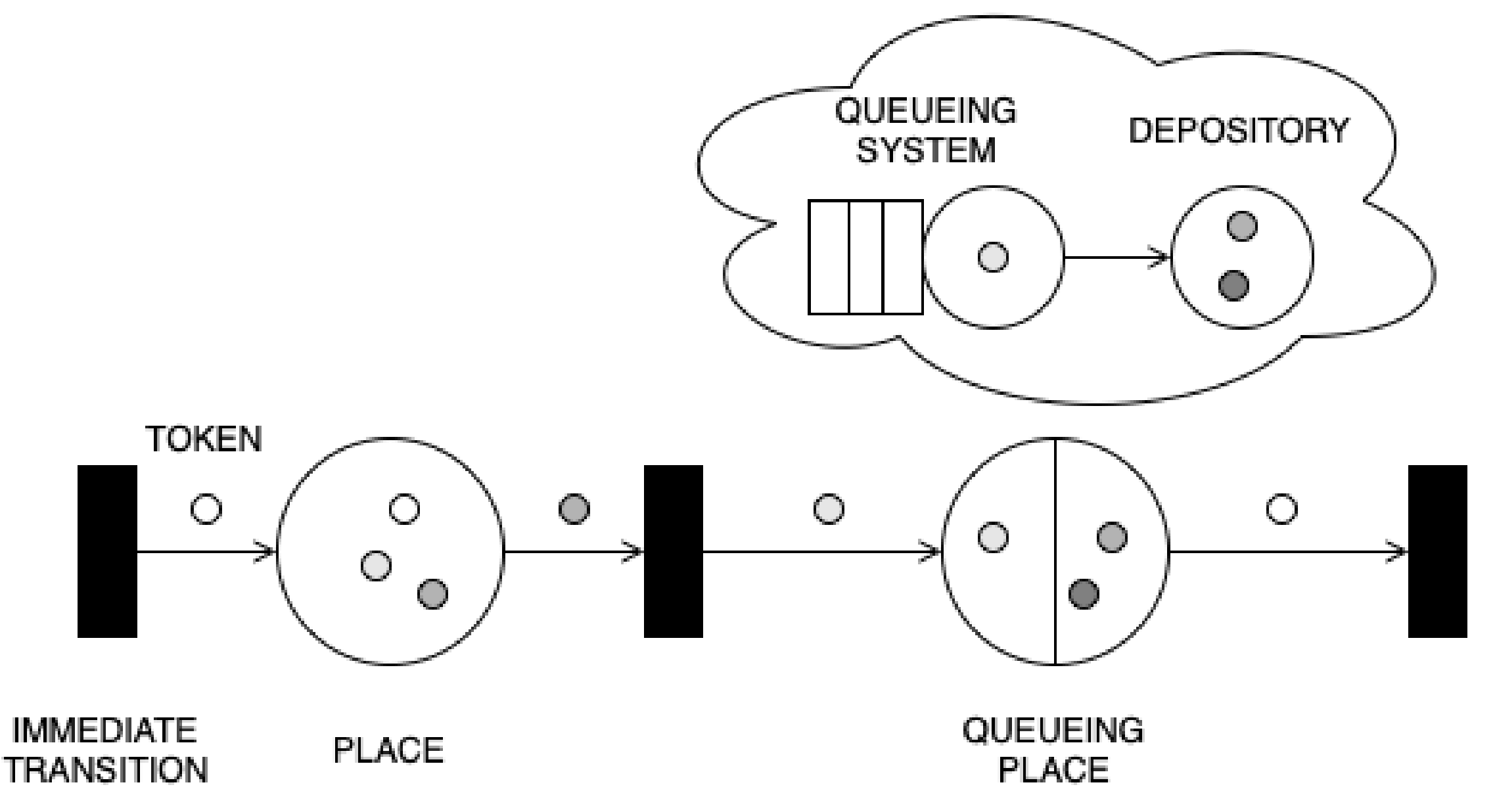
QPNs can be seen as an extension of stochastic PNs. The main idea of QPNs is to add queueing and timing aspects to the net places and timed transitions. QPNs allow queues to be integrated into the places of a PN. Places (QPN) are divided into two types: ordinary and queued. A place that contains an integrated queue is called a queueing place. Queueing places contain two components: the queue and the depository of tokens that complete their service at a queue. Tokens are used to model requests and enter the queueing place through the firing of input transitions. The different possibilities of firing a transition are referred to as modes. Modes have firing weights (probabilities) that influence which mode is chosen. Tokens are inserted into a queueing place according to the queue’s scheduling strategy. Timed queueing places have service distributions. In the queueing place, if a server is available, arriving tokens are first serviced. If a server is not available, the tokens have to wait in the waiting area. The time it takes to service a token is defined through a statistical distribution. After service, the tokens are immediately moved to a depository, where they become available for output transitions. When a transition fires, tokens are removed from some places and new tokens are created at others. Figure 1 shows the notation used for ordinary places and queueing places. For more details, refer to [5].

Figure 1.
QPN notation.
To analyze any QPN it is necessary to determine:
- Set of places;
- Set of queueing places with scheduling strategy;
- Set of immediate or timed transitions (QPNs allow transitions to fire in different modes (transition colors));
- Initial marking (number of tokens);
- Incidence function (routing probability) is defined per color/mode basis;
- Arcs with firing weights as relative firing frequency of the mode;
- Token color function specifies the types of tokens that can reside in the place and allows transitions to fire in different modes.
The color function assigns a set of colors to each transition. Incidence functions are defined on a per color basis.
QPN model was used to check the behavior of the token and it was developed using the QPME tool [22].
2.2. Mathematical Model of QPN
In [23], the general model of QPN was defined and some symbols were introduced. This is briefly summarized in this subsection.
Queueing Petri nets have the advantages of QNs (e.g., evaluation of the system performance, the network efficiency) and PNs (e.g., logical assessment of the system correctness). The main idea of QPNs is to add queueing and timing aspects to the net places. QPN is a tuple (1).
where:
- is a finite and non-empty set of places;
- is a finite and non-empty set of transitions;
- ;
- is a color function defined from into finite and non-empty sets (specify the types of tokens that can reside in the place and allow transitions to fire in different modes);
- are the backward and forward incidence functions defined in , such that (specify the interconnections between places and transitions; the subscript denotes multisets. denotes the set of all finite multisets of );
- is an initial marking defined on , such that (specify how many tokens are contained in each place).
- , where:
- -
- is a set of timed queueing places;
- -
- is a set of immediate queueing places;
- -
- ;
- -
- is an array with a description of places (if is a queueing place, denotes the description of a queue with all colors of into consideration, or if is the ordinary place () equals ).
- , where:
- -
- is a set of timed transitions;
- -
- is a set of immediate transitions;
- -
- , ;
- -
- is an array (entry , such that ) of:
- *
- rate of a negative exponential distribution specifying the firing delay due to color , if ;
- *
- firing weight specifying the relative firing frequency due to color , if .
2.3. Stream Generator
In this article, we present the modified version of the SG model shown in [7], which is based on QPNs. This is a simple way to model a user stream, who generates requests transferred to the system.
The model allows us to freely join the or user tokens with the or resource tokens. Thus, any distribution in can be obtained in this way.
The logic lies in the firing of transitions with weights and handling of the token colors. The following cases are considered:
- In a simple SG, any user can use any resource in the stream generation process.
- In other cases, any stream can be generated based on a predetermined weight value.
We get the populations with the expected distribution of the output stream (approximately):
- Simple model ;
- Varied models, e.g., ; ; ; ; ; , ; .
The stream preparation technique presented here provides a framework for a model that can be used in system performance modeling. For technical details on the simulation tool, we refer the reader to [22].
3. Testing in QPME Tool
Every system model could be divided into parts: the client and the system [9]. We started modeling the first part, called SG.
3.1. Mathematical Model of SG in QPN
- Set of places .
- Set of transitions .
- Color function for colors . where:
- -
- and -user-classes;
- -
- and -resources;
- -
- , , , -stream.
- Incidence functions specify the interconnections between places and transitions .
- Initial marking specify how many tokens are contained in each place .
- , where:
- -
- ;
- -
- ;
- , where:
- -
- ;
- -
- , where the transition is immediate;
- -
- , for simple model and for exemplary varied models , , , , , , , where:
- *
- Color function ;
- *
- Colors ;
- *
- transition modes .
3.2. Simulation Model
The SG model is shown in Figure 2. SG is represented in the model by a set of places ( and ), queueing place (), and immediate transition (All transition cases of the model are shown in Table 1). Table 2 provides details on the places used in the model. Requests and resources are modeled by tokens of different colors. generates tokens of user requests and at the given rate. generates different available resources as or tokens. Every request goes to the system. After acquiring a resource or from the place, the requests are placed into the place of the model. The place consists of , , , and tokens. In Table 1 we concentrate only on the place and generated new tokens. Table 3 defines the token colors that we use.
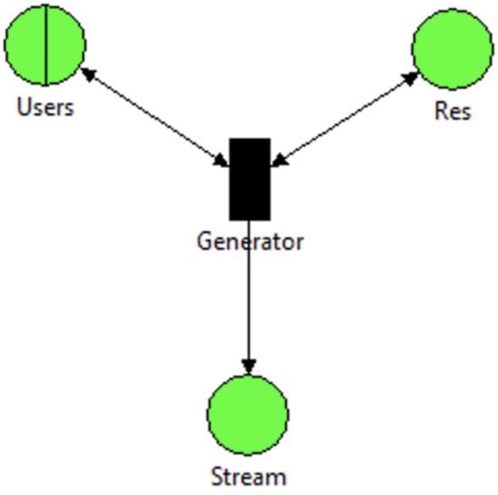
Figure 2.
SG model.

Table 1.
Firing modes of transition.
Table 2.
Places used in the model.
Table 3.
Token colors.
The used queue is described by Kendall notation (), where A denotes the probability distribution function that specifies the interarrival time of tokens (−means different requests interarrival time), B is the probability distribution function of a service time (M means exponential (Markovian) distribution of the request service time), K determines the maximum number of requests that can arrive in a queue (in this case, it is ∞) and L-scheduling strategy (in this case, it is the infinite server).
has an infinite server queue with an initial population of request tokens. The transition is configured to fire these tokens into the system (modeled as place). Firing the transition (Figure 3) creates a token in the place, assigns one of the resources to one of the users. is an ordinary place that contains the resulting stream of the mean token population.
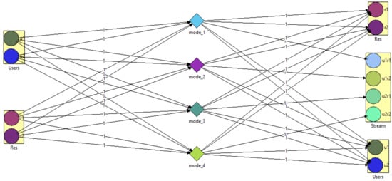
Figure 3.
Incidence function.
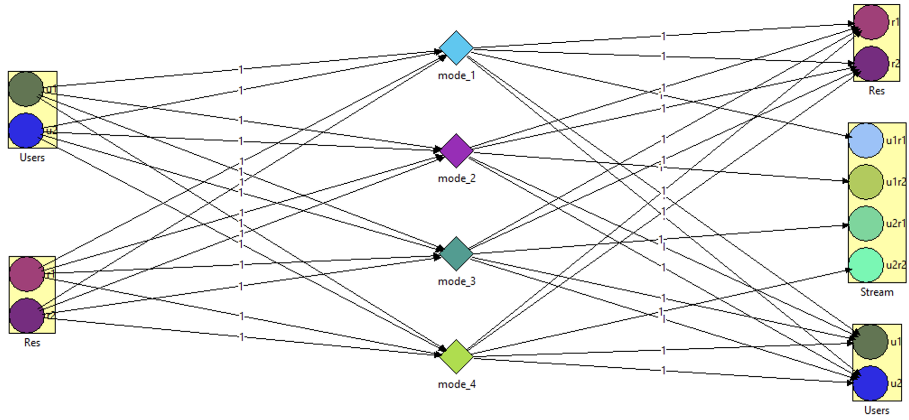
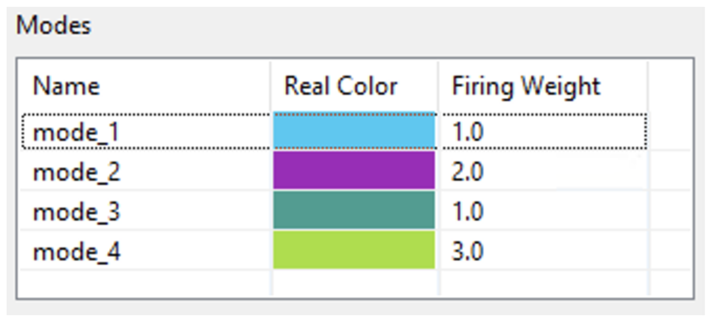
The method used to model restrictions of the user/resource mapping involves the appropriate selection of firing weights (Figure 4). In this model, tokens are generated based on this value. We assign different firing weights to the prepared modes of these transitions so that they have various probabilities of being fired when multiples of them are enabled at the same time. We use the notation (3) to denote firing modes (Table 1) (The symbols and are used here to refer to the input and output places of transitions, respectively). After the token is destroyed in an input place by the transition , a new token is created in an output place.
where:
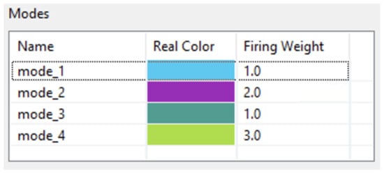
Figure 4.
Transition modes.
- A c token is removed from place ;
- A token is deposited in place .
The modeling approach was tested with different input firing weight values to demonstrate its effectiveness and practical applicability.
4. Stream Generator Results
In this section, we present an evaluation of our modeling approach. In many models, it is typical to distribute the data in random order. However, we need predefined distributions in some cases. The modeling approach was described in the previous section, and it allows simulating any input data distribution. The QPME tool generates a report showing the predicted SG population for the individual model configuration.
Table 4 and Table 5 present the results for each token in place. We can find the mean token population for place. Table 4 shows the token population for a simple case with firing weights equal for every mode (, , , ). We observe that, as expected, the mean token population is evenly distributed for tokens (, , , ). The first four lines of Table 5 show the token population for the case with firing weights equal to , , , and for individual modes. Other examples can be found in the following lines of Table 5. In all cases, the sum of all tokens in place is about 100,000, as shown in Table 4 and Table 5.
Table 4.
Token colors (simple model).
Table 5.
Token colors (varied models).
It can be observed that the quantities of the generated tokens in the place for each mode i are consistent with the appropriate firing weights w. This relation for n modes can be denoted as follows (4).
Thus, various distributions of the tokens in the stream can easily be modeled by appropriate changes in the firing weights, according to the designer’s needs. The model is general and covers special cases where one of the users is not allowed to use a particular resource. This restriction is modeled by setting the appropriate firing weight to zero.
5. Conclusions
In this paper, we used queueing Petri net formalism as an analysis technique to prepare the SG of incoming requests in the early phases of system development. Performance engineering is a field of study that solves performance problems using simulators. This field suffers from a lack of guidelines and software solutions for client behavior modeling. Modeling a system and performance analysis in the early stages of system construction ensures the best performance. This approach is a complex modeling tool for a proper selection input stream to the modeled system.
Various models of SG in miscellaneous classes of Petri nets may be considered. Our approach gradually evolves from CPN into QPN. Transition modes and firing weights, which are distinctive elements of QPN formalism, are beneficial. They can be used to model the probability of choosing appropriate binding of the transition; thus, manifold distributions of the tokens in the output stream can be generated in a comprehensive, logical manner. The model of SG presented in Section 3 is simple but flexible, able to produce the stream according to the designer’s needs, as shown in Section 4.
In this paper, the system client was taken into account. Its original design was performed using QPN models. Future research might confirm that the specific client behavior could be achieved by developing a model with a proposed SG.
Author Contributions
Writing—original CPN model, D.R.; writing—original QPN model, T.R. All authors have read and agreed to the published version of the manuscript.
Funding
This research received no external funding.
Conflicts of Interest
The authors declare no conflict of interest.
References
- Zatwarnicki, K.; Barton, S.; Mainka, D. Acquisition and Modeling of Website Parameters. In Advanced Information Networking and Applications-Proceedings of the 35th International Conference on Advanced Information Networking and Applications (AINA-2021), Toronto, ON, Canada, 12–14 May 2021; Volume 3; Barolli, L., Woungang, I., Enokido, T., Eds.; Lecture Notes in Networks and Systems; Springer: Berlin/Heidelberg, Germany, 2021; Volume 227, pp. 594–605. [Google Scholar] [CrossRef]
- Krajewska, A. Performance Modeling of Database Systems: A Survey. J. Telecommun. Inf. Technol. 2019, 8, 37–45. [Google Scholar] [CrossRef]
- Cherbal, S. Load balancing mechanism using Mobile agents. Informatica 2021, 45, 257–266. [Google Scholar] [CrossRef]
- Walid, B.; Kloul, L. Formal Models for Safety and Performance Analysis of a Data Center System. Reliab. Eng. Syst. Saf. 2019, 193, 106643. [Google Scholar] [CrossRef]
- Rak, T. Formal Techniques for Simulations of Distributed Web System Models. In Cognitive Informatics and Soft Computing; Mallick, P.K., Bhoi, A.K., Marques, G., Hugo, C., de Albuquerque, V., Eds.; Springer: Singapore, 2021; pp. 365–380. [Google Scholar] [CrossRef]
- Fiuk, M.; Czachórski, T. A Queueing Model and Performance Analysis of UPnP/HTTP Client Server Interactions in Networked Control Systems. In Computer Networks (CN 2019); Communications in Computer and Information Science; Springer International Publishing AG: Cham, Switzerland, 2019; pp. 366–386. [Google Scholar] [CrossRef]
- Rzonca, D.; Rzasa, W.; Samolej, S. Consequences of the Form of Restrictions in Coloured Petri Net Models for Behaviour of Arrival Stream Generator Used in Performance Evaluation. In Computer Networks; Gaj, P., Sawicki, M., Suchacka, G., Kwiecień, A., Eds.; Springer International Publishing: Cham, Switzerland, 2018; pp. 300–310. [Google Scholar] [CrossRef]
- Kounev, S.; Lange, K.D.; von Kistowski, J. Systems Benchmarking: For Scientists and Engineers; Springer International Publishing: Cham, Switzerland, 2020. [Google Scholar] [CrossRef]
- Rak, T. Modeling Web Client and System Behavior. Information 2020, 11, 337. [Google Scholar] [CrossRef]
- Rak, T. Performance Modeling Using Queueing Petri Nets. In Computer Networks (CN 2017); Gaj, P., Kwiecien, A., Sawicki, M., Eds.; Communications in Computer and Information Science; Springer International Publishing AG: Cham, Switzerland, 2017; Volume 718, pp. 321–335. [Google Scholar] [CrossRef]
- Zatwarnicki, K. Providing Predictable Quality of Service in a Cloud-Based Web System. Appl. Sci. 2021, 11, 2896. [Google Scholar] [CrossRef]
- Eismann, S.; Grohmann, J.; Walter, J.; von Kistowski, J.; Kounev, S. Integrating Statistical Response Time Models in Architectural Performance Models. In Proceedings of the 2019 IEEE International Conference on Software Architecture (ICSA), Hamburg, Germany, 25–29 March 2019; pp. 71–80. [Google Scholar] [CrossRef]
- Roshany, M.; Khorsandi, S. Performance analysis of the internet-protocol multimedia-subsystem’s control layer using a detailed queueing Petri-net model. Int. J. Commun. Syst. 2018, 32, e3885. [Google Scholar] [CrossRef]
- Curiel, M.; Pont, A. Workload Generators for Web-Based Systems: Characteristics, Current Status, and Challenges. IEEE Commun. Surv. Tutor. 2018, 20, 1526–1546. [Google Scholar] [CrossRef]
- Kolbusz, J.; Paszczynski, S.; Wilamowski, B. Network traffic model for industrial environment. In Proceedings of the 2005 3rd IEEE International Conference on Industrial Informatics (INDIN’05), Perth, Australia, 10–12 August 2005; pp. 406–411. [Google Scholar] [CrossRef]
- Tang, W.; Fu, Y.; Cherkasova, L.; Vahdat, A. Modeling and generating realistic streaming media server workloads. Comput. Netw. 2007, 51, 336–356. [Google Scholar] [CrossRef]
- Lukichev, M. Formation of equivalent simulation model of an real-time video stream generator used in packet-oriented communication networks, taking into account the structure of the H.264 compression algorithm. T-Comm 2019, 13, 43–52. [Google Scholar]
- Samolej, S.; Szmuc, T. HTCPNs–Based Tool for Web–Server Clusters Development. In Software Engineering Techniques; Huzar, Z., Koci, R., Meyer, B., Walter, B., Zendulka, J., Eds.; Springer: Berlin/Heidelberg, Germany, 2011; pp. 131–142. [Google Scholar]
- Samolej, S.; Szmuc, T. Web–Server Systems HTCPNs-Based Development Tool Application in Load Balance Modelling. e-Inform. Softw. Eng. J. 2009, 3, 139–153. [Google Scholar]
- Bause, F.; Buchholz, P.; Kemper, P. Hierarchically Combined Queueing Petri Nets; Springer: Berlin/Heidelberg, Germany, 2006; pp. 176–182. [Google Scholar] [CrossRef]
- Kounev, S.; Spinner, S.; Meier, P. Introduction to queueing petri nets: Modeling formalism, tool support and case studies. In Proceedings of the 3rd Joint WOSP/SIPEW International Conference on Performance Engineering (ICPE’12), Boston, MA, USA, 22–25 April 2012. [Google Scholar] [CrossRef]
- Kounev, S.; Spinner, S.; Meier, P. QPME 2.0—A Tool for Stochastic Modeling and Analysis Using Queueing Petri Nets; Springer: Berlin/Heidelberg, Germany, 2010; Volume 6462, pp. 293–311. [Google Scholar] [CrossRef]
- Rak, T. Response Time Analysis of Distributed Web Systems Using QPNs. Math. Probl. Eng. 2015. [Google Scholar] [CrossRef] [Green Version]

Publisher’s Note: MDPI stays neutral with regard to jurisdictional claims in published maps and institutional affiliations. |
© 2021 by the authors. Licensee MDPI, Basel, Switzerland. This article is an open access article distributed under the terms and conditions of the Creative Commons Attribution (CC BY) license (https://creativecommons.org/licenses/by/4.0/).