Abstract
Relay-aided free-space optical (FSO) communication systems have the ability of mitigating the adverse effects of link disruption by dividing a long link into several short links. In order to solve the relay selection (RS) problem in a decode and forward (DF) relay-aided FSO system, we model the relay selection scheme as a Markov decision process (MDP). Based on a dueling deep Q-network (DQN), the DQN-RS algorithm is proposed, which aims at maximizing the average capacity. Different from relevant works, the switching loss between relay nodes is considered. Thanks to the advantage of maximizing cumulative rewards by deep reinforcement learning (DRL), our simulation results demonstrate that the proposed DQN-RS algorithm outperforms the traditional greedy method.
1. Introduction
Over the past few years, free-space optical (FSO) communications have attracted considerable attention, becoming an interesting alternative for next-generation broadband. Compared with conventional radio-frequency (RF) systems, the FSO system has the advantages of license-free transmissions, large bandwidth, simple and inexpensive implementation, and high-rate transmission capability [1,2,3].
Despite these appealing features, there are also some inevitable challenges hampering the system performance when transmitting through the atmosphere. Typical degradations include atmospheric turbulence-induced fading, geometrical loss and pointing errors [4]. As a result, the transmission distance and system performance are limited significantly. To overcome this limitation, relaying techniques are investigated by dividing a long link into several short links [5]. The utilization of relays can also remove the requirement that the source node and the destination node be in line of sight.
1.1. Related Works
To the best of the authors’ knowledge, the existing works on cooperative relaying FSO systems can be divided into two categories, which are performance analysis and optimization algorithms. In the first category, the system indexes are analyzed and derived, including bit error rate (BER) or symbol error rate (SER) [6,7], outage probability (OP) [8], channel capacity [9,10].
In the second category, studies on optimization algorithms can be viewed as an extension of the first category, where the abovementioned system indexes are either maximized or minimized by optimizing parameters including power allocation [11,12], relay placement [13,14] and relay selection [5,15,16,17]. Since this paper focuses on the relay selection issue, the related papers are analyzed. It should be mentioned that either channel state information (CSI) or partial CSI is assumed to be a priori information during the optimization algorithms, which can be estimated or obtained due to the quasi-static channel.
Ref. [5] has discovered that the best relay can be selected to minimize the BER, according to the channel conditions in source to the relay (S-R) link, the relay to destination (R-D) link and the source to destination (S-D) link. A comprehensive comparison was carried out between three cases, i.e., proactive relay, reactive relays and direct link. In Ref. [15], a relay selection algorithm was proposed as a solution to mitigate channel fading, where two cooperative modes enhanced network capacity, i.e., the intra-relay set and inter-relay set cooperative modes. A link scheduling algorithm was further proposed to improve bandwidth utilization and reduce the occupancy rate of the transceivers by better utilizing the idle FSO links. Ref. [16] investigated a new distributed relay selection algorithm where each relay was allowed to transmit only when its SNR was higher than a given threshold. The threshold was achieved with the gradient algorithm to guarantee the lowest SER. Ref. [17] proposed an improvement to the existing S-R protocol by relay selection, which was better tailored to realistic systems deploying finite-size buffers. It was shown that the proposed scheme could enhance the diversity order without the need of implementing buffers of infinite size that cause infinite delays. The closed-form asymptotic expressions of OP for two-relay networks were also derived.
With the development and application of machine learning (ML), ML-based relay selection algorithms have become a hot topic. In Ref. [18], a supervised ML-enabling scheme was proposed in order to enable a combined relay selection to avoid high computing latency. In Ref. [19], a model-free primal-dual deep learning algorithm was designed to increase the transmission capacity, and the policy gradient method was applied to the primal update in order to estimate the necessary gradient information. Ref. [20] modeled the CSI in the process of cooperative communications with relay selection as a Markov decision process. A deep Q-network (DQN) was employed to choose the optimal relay from a plurality of relay nodes, where both the outage probability and mutual information were the objective function.
It should be noted that the difference between Refs. [18,19,20] is that Ref. [18] employed a supervised learning structure, while Refs. [19,20] utilized a reinforcement learning (RL) structure. The former learns from a labeled dataset, which provides answers that the algorithm can use to evaluate its accuracy on the training data. The latter has the ability of learning strategies to maximize rewards during interactions with the environment. Owing to the fact that the RL approach is committed to maximizing the cumulative reward, it has irreplaceable advantages in dynamic optimization problems.
1.2. Motivation and Contribution
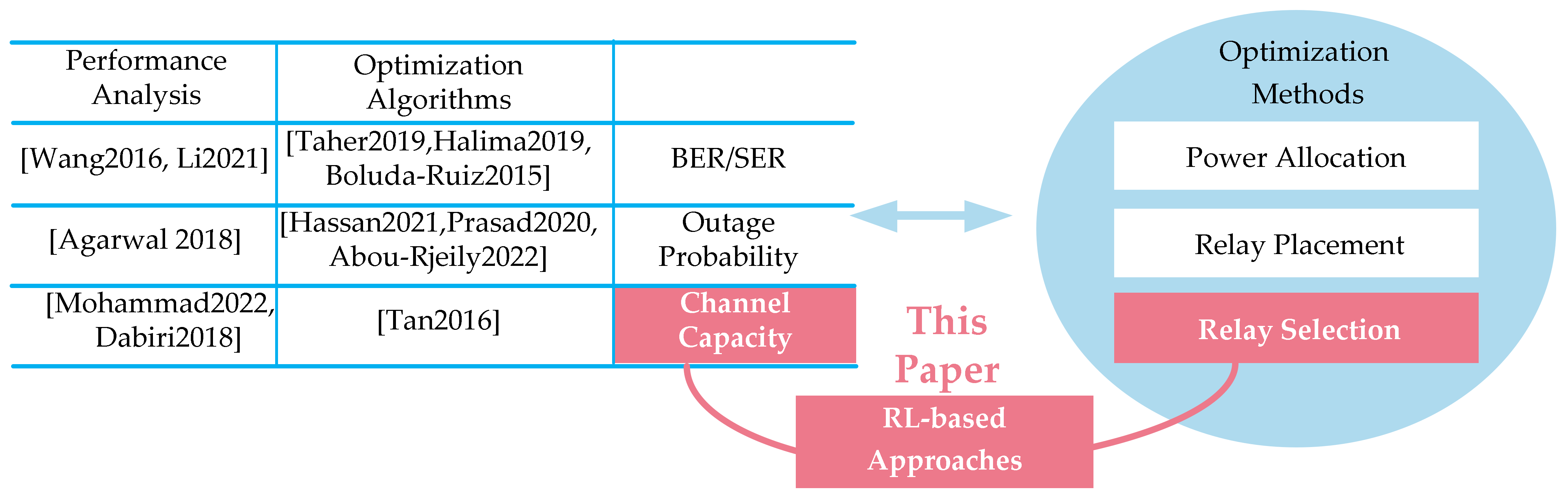
The above literature review and the research content of this paper are shown in Figure 1. Motivated by Refs. [19,20], we focus on the use of RL to solve the relay selection problem in FSO systems. We utilize the RL approach to select the relay, which aims at maximizing the channel capacity.

Figure 1.
Literature review and the research content of this paper.
As a result, we have to choose the most appropriate algorithm from the RL family. There are three main algorithms in the RL family, which are Q-learning, DQN, and deep deterministic policy gradient (DDPG) [21]. Q-learning deals with the discrete states and actions, DDPG has an actor-critic architecture that handles the continuous action and state spaces, whereas in the DQN algorithm, the action space is discrete, while the state space is continuous.
In relation to our relay selection problem, the agent chooses the best action after observing the current environment state. The action consists in selecting the appropriate relay, while the state includes both the previous selected relay and the current CSI. DQN appeared as the most appropriate method. As a result, this study employed the dueling-DQN approach to select the relay in order to maximize the channel capacity, where the relay nodes acted as the decode-and-forward (DF) mode, i.e., a cooperative DF-FSO. The main contributions of this study are as follows.
- A Markov Decision Process (MDP) model was developed to describe the relay selection problem.
- Different from the abovementioned literature, the switching loss between relay nodes was considered. The corresponding expression of channel capacity was also derived.
- We propose a DQN-RS algorithm based on the dueling DQN method, which deals with the relay selection issue in a cooperative DF-FSO system in order to achieve higher channel capacity.
- In our proposed DQN-RS algorithm, a state contained both the previous selected relay and the current CSI. An action presented the current selected relay, where the corresponding reward was equal to the derived channel capacity.
1.3. Paper Structure
The remainder of this paper is organized as follows. The system model and problem formulation are presented in Section 2. The proposed DQN-RS algorithm is illustrated in Section 3. We provide simulation results in Section 4. The conclusions and prospects are reported in Section 5. The variables are illustrated in lowercase italic, and all vectors are in lowercase bold form.
2. System Structure and Problem Formulation
This section is divided into two subsections. In Section 2.1, the system structure is illustrated, consisting of both system model and channel capacity’s expression. In Section 2.2, we first updated the expression of channel capacity by introducing the switching loss. The problem to be optimized is further shown in a mathematical manner.
2.1. System Structure
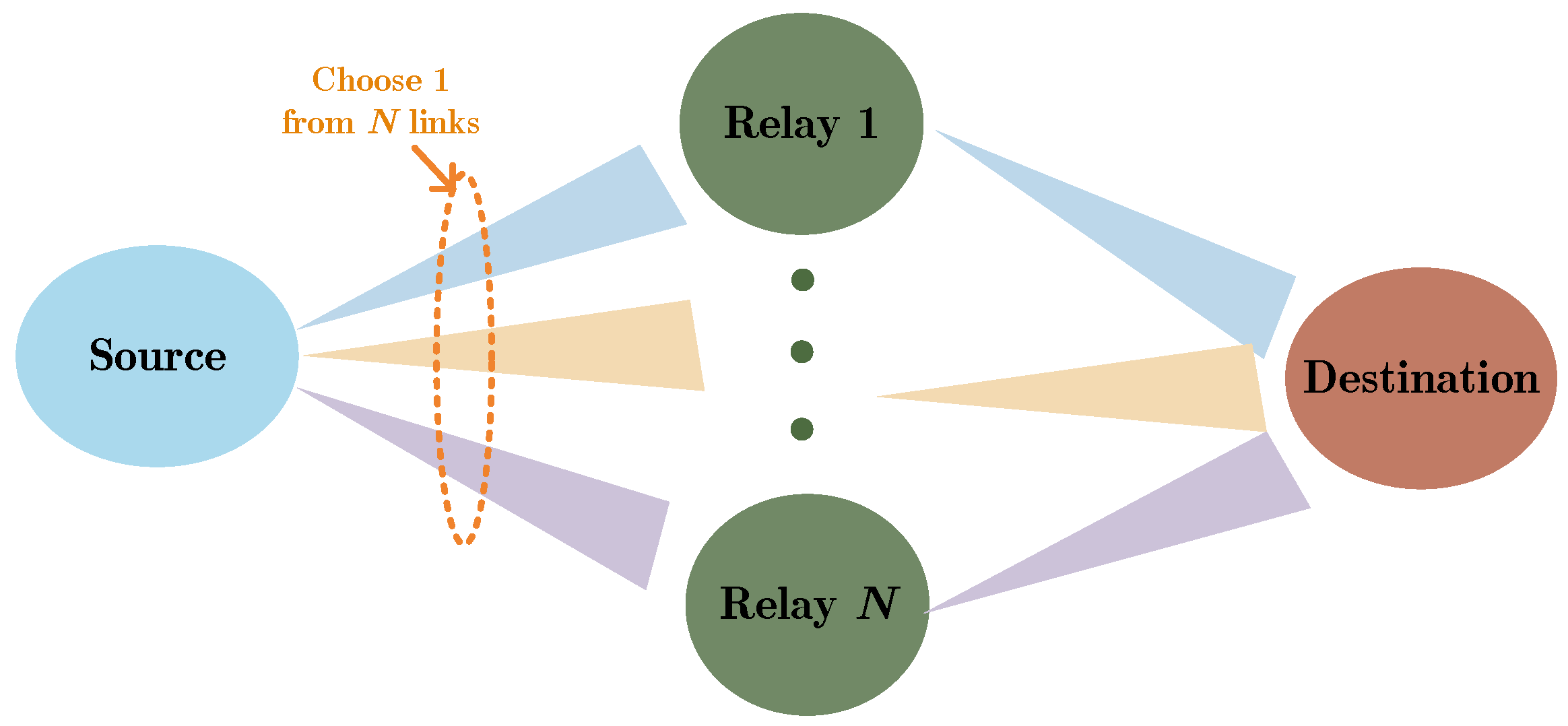
In this paper, we consider a relay-assisted FSO system in DF mode, i.e., a cooperative DF-FSO system, as shown in Figure 2. A cooperative DF-FSO system contains one source node, one destination node and relay nodes. In order to achieve higher received power, the narrow divergence angle technique is always utilized in FSO systems. In this sequel, it common that only one relay node can receive the signals from the source node in each time slot (TS), which is selected by switching the direction of the transmit beam. According to Ref. [22], optical switches can be implemented with either spatial light modulators (SLM) or optical micro-electromechanical systems (MEMS). Correspondingly, the selected relay node decodes and forwards the received signal to the destination node, which forms the R-D link.
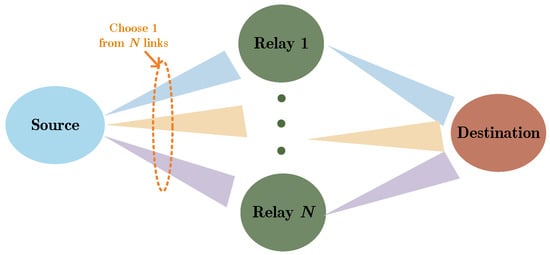
Figure 2.
System structure of a DF-FSO system.
In an arbitrary -th TS, it is supposed that the -th relay node is selected. Then, the channel capacity of a cooperative DF-FSO system can be expressed by Equation (1), where the intensity modulation/direct detection (IM/DD) is employed:
where denotes the photodetector responsivity, and represent the variance of the equivalent noise in S-R link and R-D link, respectively, is the transmitting power in the source node and the selected relay node, and stand for the channel gains from the source node to the -th relay node and from the -th relay node to the destination node, respectively. Then, vector is defined as the sets of CSI in all S-R links in the -th TS, i.e., . Similarly, vector is defined as , representing the sets of CSI of R-D links in the -th TS. According to Ref. [5], the channel gain contains both the turbulent fading and the pointing errors, whose PDF (probability density function) is described with Equation (2):
where stands for the Meijer’ G function, and represent the effective numbers of large-scale or small-scale turbulent eddies respectively, which describe the Gamma–Gamma distribution, stands for the ratio between the equivalent beam radius and the standard deviation of the pointing errors, is the maximum fraction of the collected power in the receiving lens.
2.2. Problem Formulation
Different from relevant relay selection schemes, this paper considers the switching loss when switching between the different relay nodes, which is a realistic consideration. For convenience of representation, we assume that the duration of each time slot was normalized to 1. We define as the switching loss when switching between neighboring relays. It is also assumed that the switching process is operated at a constant angular speed. That is to say, the switching loss between the -th relay node and the -th relay node is calculated by . Apparently, the switching loss from the -th relay to the -th relay will be equal to the switching loss from the -th relay to the -th relay. In addition, the switching time is equal to zero when the same relay node is selected in both current and previous TS.
The S-R link and the R-D link cannot transmit data before the switching process is completed. In other words, the switching process will reduce the available time of communication, which limits the channel capacity. As a result, considering the switching loss, the channel capacity of the -th TS was modified in Equation (3).
This paper focused on maximizing the average channel capacity over time slots, as shown in Equation (4):
where stands for the sets of the selected relays, i.e., .
Obviously, this exhaustive method can solve this problem if the CSI of all slots are available. However, this is unachievable, since the future CSI could not be known. In addition, the complexity of the exhaustive method grows exponentially as the number of TS increases, which is unacceptable. Regarding Equation (4), the system needed to select the current relay cautiously, since every choice might change the future channel capacity. As a result, we have to choose every relay by taking into account the possible impact on the future channel capacity. Fortunately, we could employ RL method, which aims at maximizing the long-term cumulative rewards.
3. DRL-Based Solution
In this section, there are three subsections. In Section 3.1, we first introduce the reasons behind using RL frameworks to solve the formulated optimization problem. The channel capacity to be optimized was further converted into the cumulative reward in the RL-frameworks. In Section 3.2, the formulated optimization problem is modeled as an incompletely known MDP, and the concept of Q-function is introduced. In Section 3.3, our proposed DQN-RS is illustrated in detail.
3.1. RL Framework-Based Optimization Problem
As illustrated above, the main purpose of this study is to maximize a long-term average channel capacity. Every relay selection will have an impact on the capacity in the following TSs. As a result, long-term cumulative rewards should be maximized in each TS. This agrees with the fact that RL approaches can maximize cumulative rewards. We defined the discounted cumulative capacity from -th TS as follows:
where represents the discount factor ranging from 0 to 1.
As a result, we formulate the cumulative capacity maximization problem as
3.2. Markov Decision Process
In this subsection, we investigate an RL framework to solve our optimization problem described in Equation (6), where the agent learns to select the optimal relay to obtain the largest cumulative reward. The problem of RL is formulized as the incompletely known MDP. On the basis of the Markov property, the next state of a system is only related to the current state and the current selected action, and it is independent of earlier states.
An MDP always consists of a four-tuple, namely, , where denotes the state space, represents the action space, is the immediate reward function, and is the transition probability. It has to be considered that statistical knowledge over the model-free environment is not available. In our problem, the state transition probability was unknown. Thus, the detailed physical meaning of is illustrated.
- State Space: The current state space of the whole system at the -th TS is defined as , which consists both the previous selected relay node and the current CSI. represents the selected relay in the -th TS by one-hot code.
- Action Space: In our system model, the agent, as the decision maker, makes an optimal decision on the relay selection. The current action space of the whole system at -th TS is defined as .
- Immediate reward function: After taking action in state , the system will transfer to the next state ; meanwhile, the agent will obtain an immediate reward . In our optimization problem, the immediate reward was defined as the current capacity defined in Equation (3), i.e., .
In RL tasks, an agent learns an optimal strategy to maximize the expected discounted future cumulative reward in Equation (5). In order to measure the quality of any arbitrary strategy , the value function is introduced, which is defined to be the expected discounted cumulative reward in the future as the long-term reward by executing an action in an environmental state , i.e., . The value function can be expressed in a recursive form, as shown in Equation (7), which is always called the Bellman equation.
So far, finding an optimal policy in RL tasks means to solve the above Bellman equation. To achieve this goal, we just transferred our optimization objective in Equation (7). Our DRL-based algorithms to solve this equation is presented in the following subsection.
It needs to be mentioned that the markers , only used to explain MDP, indicate the whole sets of state space, action space and reward space, while the marker s (or a; r) denotes an arbitrary element belonging to the corresponding set. The markers stand for the instantaneous element in the -th time slot in the proposed DQN-RS algorithm.
3.3. The DQN-RS Algorithm
The simplest RL tasks, where the state and action spaces are small enough for the state action values, i.e., the Q-values to be represented as tables, can be solved by a regular Q-learning method. In this paper, we try to solve a relay selection problem in a cooperative DF-FSO system with continuous state and discrete action space. Under this circumstance, it is impractical to maintain all Q-values. Hence, we use an approximate solution method that can be applied effectively to complex problems. The DQN algorithm is a typical algorithm based on the value-based approximation method, which uses some neural networks to approximate the action value function and can learn finite discrete values from a high-dimensional state space and output action with the highest action value.
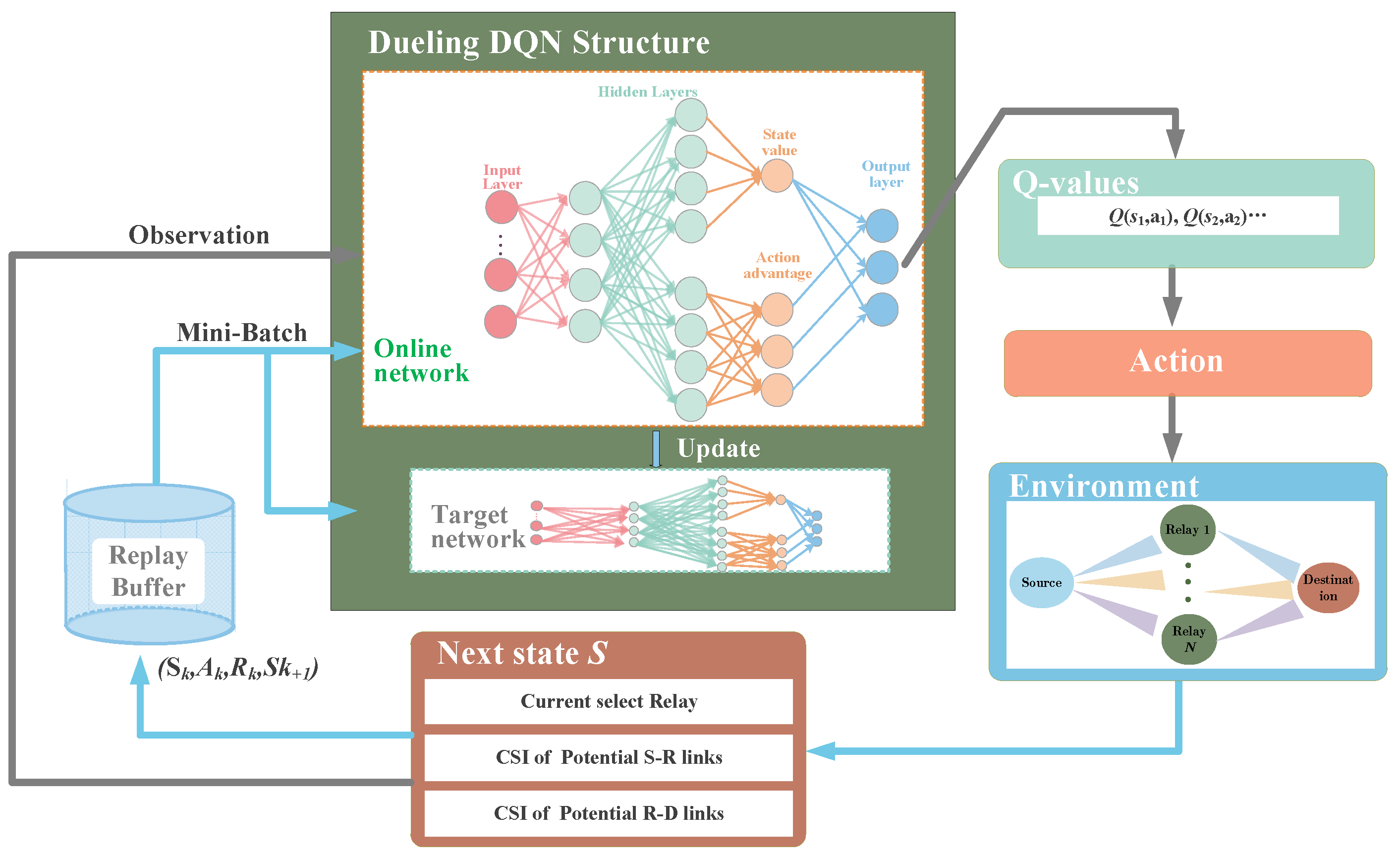
The dueling DQN improves the algorithm performance by optimizing the neural network structure [23]. In this way, the Q-values are more robust and can be estimated with lower variance. The architecture of our proposed dueling DQN-based DQN-RS algorithm is shown in Figure 3.

Figure 3.
Proposed DQN-RS algorithm framework.
As can be seen in Figure 3, our DQN-RS framework consists of two neural networks. One is the online network, the other is the target network, and both share the same structure. Different from the conventional DQN which directly estimates the Q-values by one stream, the dueling architecture consists of two streams of fully connected layers that represent state value and action advantage , respectively, while sharing common feature layers. Then, the two streams are combined via a special aggregating layer to produce the estimated Q-values. After estimating these Q-values, the agent can choose the action with the highest Q value, i.e., select the current relay. As the action is completed, the environment changes in the next time slot, which corresponds to the change of state in the new slot. The state can be observed by the agent as the input to the DQN-RS networks. Our proposed algorithm proceeds in an iterative manner according to the process described above. As shown in Figure 3, a replay buffer storing experience data is used to train the two networks.
The motivation for using this dueling DQN structure is to solve the observability problem in conventional DQN. For some states, such as the channel information in our system model, their next states will not be affected by the taken actions at the current time step. Hence, it is desirable to estimate independently of . We define and in Equations (8) and (9)
where denotes the parameters of the convolutional layers, and are the parameters of the two streams of fully connected layers. Then, state action value function or Q-value function in the dueling DQN algorithm can be expressed as:
In our system, in order to improve the performance of our algorithm, we calculate the Q-value by:
where the number of elements is indicated by .
In our proposed DQN-RS algorithm, we take the state introduced in Section 3.2 as the input. We denote the output action in the DQN-RS algorithm as . These actions are selected by the -reedy method. We randomly select from the action space with probability , otherwise the action is selected by:
The dueling DQN-based algorithm also uses a dual network structure with an online network and a target network like the conventional DQN. Meanwhile, we also introduce the experience replay buffer with capacity .
After executing the selected action at arbitrary -th time slot, the agent receives the immediate reward defined in Section 3.2 and transfers it to the next state . We continue to track the experience in a replay memory with the state transition sample data [20]. When training the network, we randomly take sets of experience data from as a minibatch of the samples. An arbitrary set of experience data in the minibatch is denoted as . Then, the loss function can be expressed as:
where , and represent the weights of the target network, which correspond to , and , respectively. Defining the learning rate as , the online network can be updated by the gradient descent method, shown in Equation (14):
where , and represent the gradient vectors of with respect to , and , respectively. The weights of the target network are then updated through the slow tracking of the learned online networks, with the learning rate to be :
Our proposed DQN-RS algorithm is summarized in Algorithm 1.
| Algorithm 1. The pseudocode diagram of the proposed DQN-RS algorithm. | |
| Input: The cooperative DF-FSO simulator and its parameters. Output: Optimal action of each time slot. | |
| 1: | Initialize experience replay memory with size . |
| 2: | Initialize , and with random weights and initialize , and by . |
| 3: | Initialize the minibatch size with . |
| 4: | for episode = 1,2… do as follows |
| 5: | Initialize the environment and observe the environment initial state . |
| 6: | for do as follows |
| 7: | Select a random action with probability or otherwise select action . |
| 8: | Execute action and receive immediate reward , observe . |
| 9: | Store the transition data in the buffer . |
| 10: | if is full, do as follows |
| 11: | Sample a random minibatch of sets of transition data from . |
| 12: | Update the online network by (14). |
| 13: | Update the target network by (15). |
| 14: | end for |
| 15: | end for |
The total algorithm complexity is defined as the product of the total time steps and the algorithm complexity of each time step. We know that the algorithm complexity of an arbitrary time step is determined by the calculation of the parameter updates in the neural network. According to [21], the computational complexity for updating all the neural network parameters is per time step, where and denote the action dimension and the number of parameters, respectively. In our proposed DQN-RS algorithm, the action dimension is . The number of parameters in the proposed algorithm can be expressed as . Therefore, the approximate complexity at each time step of the proposed DQN-RS algorithm is , which is far less than that of the exhaustive method .
4. Simulation Results
In this section, the numerical results of our proposed DQN-RS algorithm in cooperative DF-FSO systems are illustrated. The greedy relay selection is also considered as a comparison, where the relay with the best CSI is selected. The simulation parameters are presented in Table 1. The simulation results were obtained on the deep learning framework in TensorFlow 1.2.1 of Python 3.6.

Table 1.
Simulation Parameters.
As mentioned above, the number of neurons in the input layer was equal to , which was the dimension of the state space. Similarly, the number of neurons in the output layer was equal to the number of relay nodes , which coincided with the dimension of the action space. In addition, there were 200 neurons in the common feature layer, whose active function was the Relu function. There were also 200 neurons in the value layer and the action advantage layer, whose active function was the linear function in our proposed DQN-RS algorithm. We trained the deep neural networks with a minibatch size of . The replay memory capacity was equal to one-third of the total training steps. The discount factor was set to 0.9.
First, the convergence performance of the mentioned DQN-RS algorithm is illustrated. We set both the learning rates to 0.001. The channel capacity versus episodes and the loss via training steps are presented in Figure 4a,b, respectively. As shown in Figure 4a, it could be divided into three parts as the episodes increased. In the first part, the agent was busy filling the replay buffer. The training process did not start until the buffer was full around the 1333rd episode, where the second part began. During the second part, the agent learned to achieve a higher Q-value by selecting different relay nodes. In the last part, the parameter was set to 0, which means the agent had the ability of dealing with the relay selection issue. According to Figure 4b, the DQN-RS algorithm converged after 2000 steps. In addition, it can be seen in Figure 4b that the curve of the loss function presents periodic fluctuations, which resulted from the fact that a bad experience may be chosen from the replay memory during the training process.
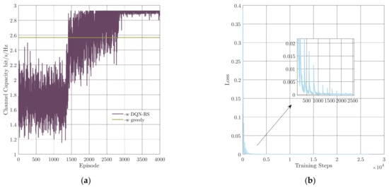
Figure 4.
Convergence performance of the proposed DQN-RS algorithm. (a) Channel capacity versus episodes, (b) loss function via training steps.
Figure 5 shows the difference of the proposed DQN-RS algorithm and the greedy algorithm; it depicts an example of relay selection in 10 TSs. As shown in Figure 5, the greedy algorithm (the green line) always choses the link with the largest channel condition, i.e., . That is why the 2nd relay node was selected in 2nd TS, rather than the 4th relay node. The greedy algorithm did not consider the switching loss. Moreover, frequent handovers would increase the time the system was unavailable, thereby reducing the channel capacity of the system, i.e., < , even though there were other relay nodes with better CSI.
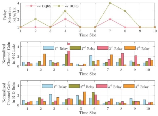
Figure 5.
An example of relay selection in 10 TSs.
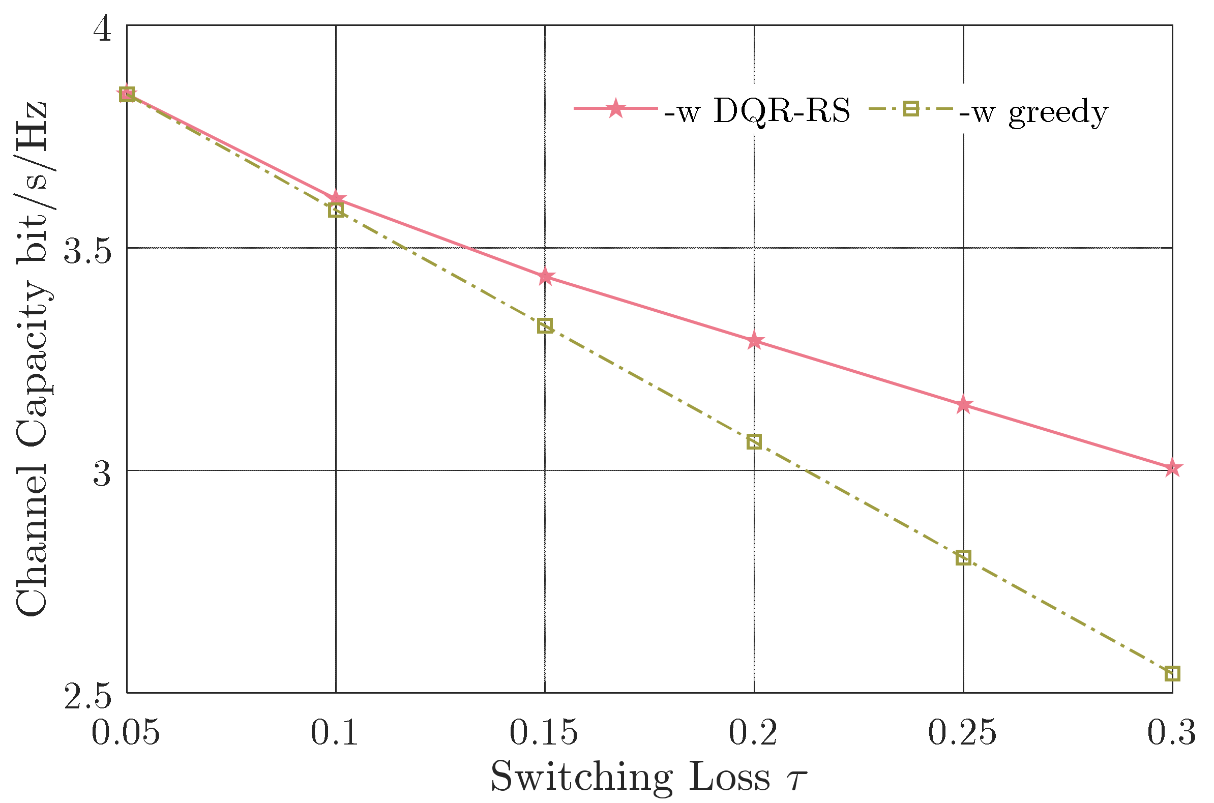
Figure 6 and Figure 7 show the average channel capacity versus different switching losses and number of relay nodes, respectively. On the basis of Figure 6, the average channel capacity decreased with a larger switching loss . This is evident because unavailable time will increase with the growth of the switching loss, when the system switches between the relay nodes. Moreover, the gap between the proposed DQN-RS scheme and the greedy algorithm became larger with the increasing switching loss. Only considering the link with the best CSI, the greedy algorithm resulted in more reps and more frequent switching between the relay nodes, which inadvertently reduced the capacity. To illustrate the effectiveness of our algorithm, we considered , defined as the capacity gain by our proposed algorithm over the greedy algorithm. In Figure 6, with the increase of the switching loss on the horizontal axis, the capacity gain could reach 18%.
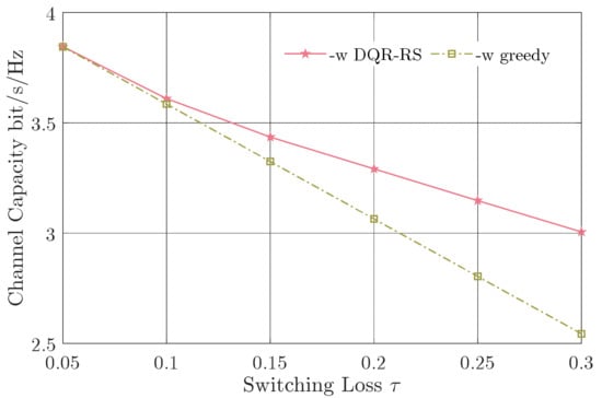
Figure 6.
Channel capacity versus switching loss .
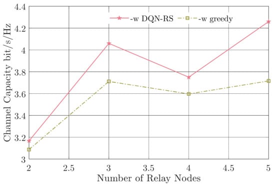
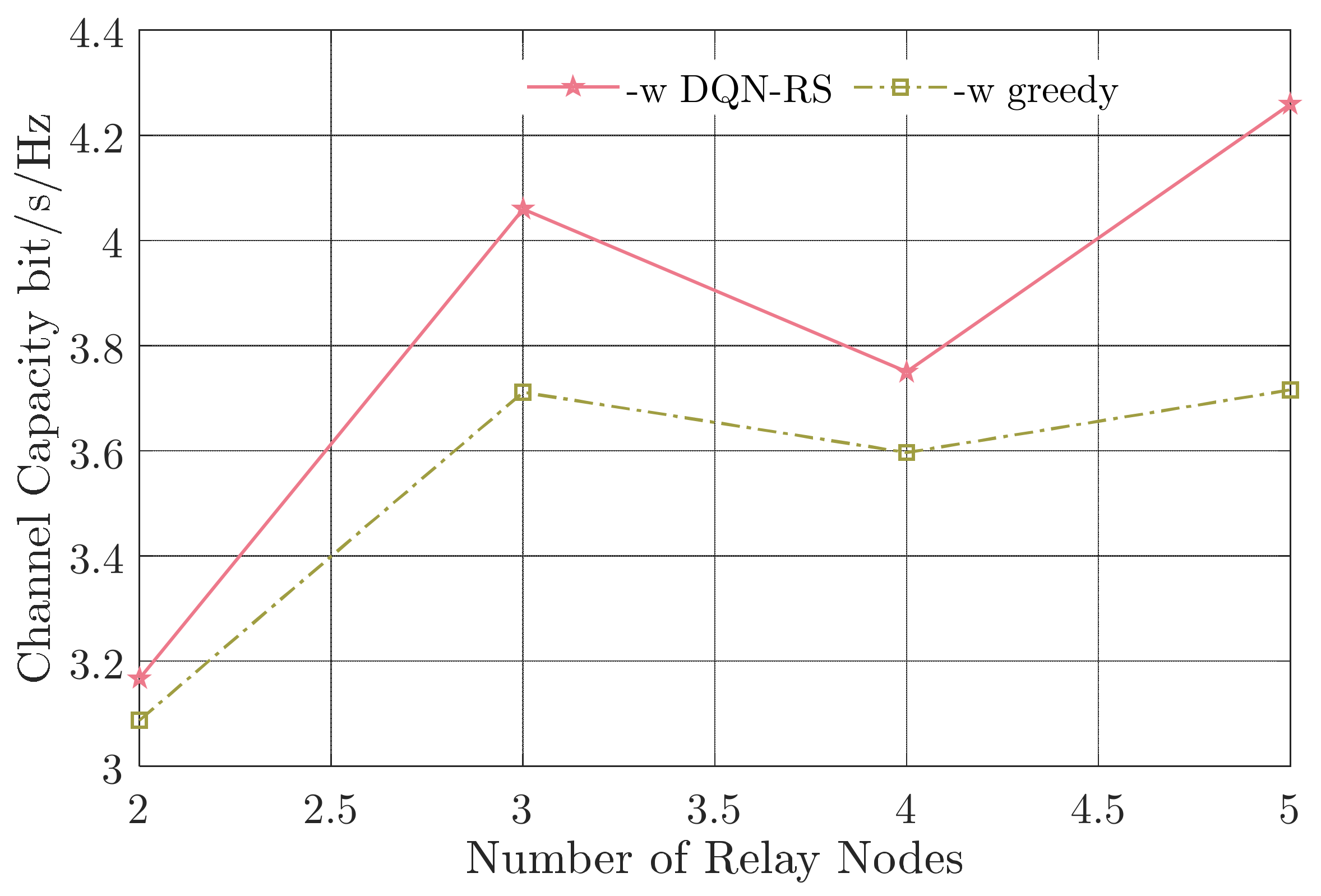
Figure 7.
Channel capacity versus the number of relay nodes.
As can be seen in Figure 7, the channel capacity did not increase monotonically with the number of the relay nodes, and the capacity gain ranged from 2.59% () to 14.6% (). It is different from the situation where there was no switching loss. As the number of relay nodes increased, the possibility of multiple links fading at the same time decreased, and there was potential to establish better channel links. However, the switching between the relay nodes would reduce the channel capacity. As a result, there was a tradeoff between the number of relay nodes and the switching loss. Therefore, the relay-aided FSO system should consider both the number of relay nodes and the switching time carefully in actual systems. It can also be concluded that our proposed DQN-RS algorithm performs better than the traditional greedy algorithm with an arbitrary number of relay nodes and different switching loss.
5. Conclusions and Prospects
In this paper, we investigated the relay selection problem in a cooperative DF-FSO system, which was modeled as a Markov decision process. A DQN-RS relay selection scheme was proposed based on the dueling DQN method, where the channel capacity was derived and maximized by considering the switching loss between the relay nodes. In our DQN-RS algorithm, a state contained both the previous selected relay and the current CSI. An action presented the current selected relay, where the corresponding reward was equal to the derived channel capacity. On the basis of the simulation results, the proposed DQN-RS algorithm outperformed the greedy method. As the switching loss increased, our algorithm became increasingly superior to the greedy method. It was also found that the channel capacity did not increase monotonically with the number of relay nodes, which is different from the traditional case where the switching loss is ignored. It indicates that there is a tradeoff between the number of relay nodes and the switching loss. In addition, it should be mentioned that our algorithm has the potential of practical application through complexity analysis.
Although both the feasibility and effectiveness of the algorithm have been verified, more work can be carried out. Two aspects of our study should be highlighted. First of all, this paper assumed that perfect channel information can be obtained. When the channel information is not perfect, how to optimize the algorithm is a topic worthy of study in order to achieve better performance. In addition, how to speed up the convergence is another point of interest. Potential improvements include, but are not limited to, optimizing the network structure and the training methods.
Author Contributions
Writing—original draft preparation, Y.-T.L.; writing—review and editing, Y.-T.L., S.-J.G. and T.-W.G.; visualization, S.-J.G. and T.-W.G.; supervision, Y.-T.L.; project administration, S.-J.G. All authors have read and agreed to the published version of the manuscript.
Funding
National Natural Science Foundation of China (NO. 62101527); Funding Program of Innovation Labs by CIOMP.
Institutional Review Board Statement
Not applicable.
Informed Consent Statement
Not applicable.
Data Availability Statement
Not applicable.
Acknowledgments
The authors also gratefully acknowledge the Optical Communication Laboratory of CIOMP for the use of their equipment.
Conflicts of Interest
The authors declare no conflict of interest.
Abbreviations
The main variables appearing in this paper are summarized below:
| channel gain from the source node to the -th relay node | |
| channel gain from the -th relay node to the destination node | |
| channel capacity of the -th TS | |
| capacity gain by our proposed algorithm over the greedy algorithm | |
| switching loss when switching between neighboring relay nodes | |
| switching loss between -th relay node and -th relay node | |
| number of relay nodes | |
| , , | parameters of the convolutional layers and two streams of fully connected layers in the online network |
| , | parameters of the convolutional layers and two streams of fully connected layers in the target network |
| , , | current state space, action space, reward of the whole system at -th TS |
| discount factor of the DQN-RS algorithm | |
| , | learning rate of the online network and target network |
References
- Al-Kinani, A.; Wang, C.X.; Zhou, L.; Zhang, W. Optical Wireless Communication Channel Measurements and Models. IEEE Commun. Surv. Tutor. 2018, 20, 1939–1962. [Google Scholar] [CrossRef]
- Zhou, H.; Fu, D.; Dong, J.; Zhang, P.; Chen, D.; Cai, X.; Li, F.; Zhang, X. Orbital angular momentum complex spectrum analyzer for vortex light based on the rotational Doppler effect. Light Sci. Appl. 2017, 6, e16251. [Google Scholar] [CrossRef] [PubMed]
- Marbel, R.; Yozevitch, R.; Grinshpoun, T.; Ben-Moshe, B. Dynamic Network Formation for FSO Satellite Communication. Appl. Sci. 2022, 12, 738. [Google Scholar] [CrossRef]
- Chauhan, I.; Bhatnagar, M.R. Performance of Transmit Aperture Selection to Mitigate Jamming. Appl. Sci. 2022, 12, 2228. [Google Scholar] [CrossRef]
- Taher, M.A.; Abaza, M.; Fedawy, M.; Aly, M.H. Relay Selection Schemes for FSO Communications over Turbulent Channels. Appl. Sci. 2019, 9, 1281. [Google Scholar] [CrossRef] [Green Version]
- Wang, P.; Wang, R.; Guo, L.; Cao, T.; Yang, Y. On the performances of relay-aided FSO system over m distribution with pointing errors in presence of various weather conditions. Opt. Commun. 2016, 367, 59–67. [Google Scholar] [CrossRef]
- Li, A.; Wang, W.; Wang, P.; Pang, W.; Qin, Y. SER performance investigation of a MPPM relay-aided FSO system with three decision thresholds over EW fading channel considering pointing errors. Opt. Commun. 2021, 487, 126803. [Google Scholar] [CrossRef]
- Agarwal, D.; Bansal, A.; Kumar, A. Analyzing selective relaying for multiple-relay–based differential DF-FSO network with pointing errors. Trans. Emerg. Telecommun. Technol. 2018, 29, e3306. [Google Scholar] [CrossRef]
- Dabiri, M.T.; Sadough, S. Performance Analysis of All-Optical Amplify and Forward Relaying Over Log-Normal FSO Channels. J. Opt. Commun. Netw. 2018, 10, 79–89. [Google Scholar] [CrossRef]
- Mohammad, T.; Nasim, M.; Chahé, N. Performance analysis of an asymmetric two-hop amplify-and-forward relaying RF–FSO system in a cognitive radio with partial relay selection. Opt. Commun. 2022, 505, 127478. [Google Scholar]
- Xing, F.; Yin, H.; Ji, X.; Leung, V. Joint Relay Selection and Power Allocation for Underwater Cooperative Optical Wireless Networks. IEEE Trans. Wirel. Commun. 2020, 19, 251–264. [Google Scholar] [CrossRef]
- Hassan, M.M.; Rather, G.M. Innovative relay selection and optimize power allocation for free space optical communication. Opt. Quant. Electron. 2021, 53, 689. [Google Scholar] [CrossRef]
- Boluda-Ruiz, R.; García-Zambrana, A.; Castillo-Vázquez, B.; Castillo-Vázquez, C. Impact of relay placement on diversity order in adaptive selective DF relay-assisted FSO communications. Opt. Express 2015, 23, 2600–2617. [Google Scholar] [CrossRef]
- Prasad, G.; Mishra, D.; Tourki, K.; Hossain, A.; Debbah, M. QoS and Energy Aware Optimal Resource Allocations in DF Relay-Assisted FSO Networks. IEEE Trans. Green Commun. Netw. 2020, 4, 914–926. [Google Scholar] [CrossRef]
- Tan, Y.; Liu, Y.; Guo, L.; Han, P. Joint relay selection and link scheduling in cooperative free-space optical system. Opt. Eng. 2016, 55, 111604. [Google Scholar] [CrossRef]
- Halima, N.B.; Boujemâa, H. Round Robin, Centralized and Distributed Relay Selection for Free Space Optical Communications. Wireless Pers. Commun. 2019, 108, 51–66. [Google Scholar] [CrossRef]
- Abou-Rjeily, C. Improved Buffer-Aided Selective Relaying for Free Space Optical Cooperative Communications. IEEE Trans. Wirel. Commun. 2022. [Google Scholar] [CrossRef]
- Dang, S.; Tang, J.; Li, J.; Wen, M.; Abdullah, S.; Li, C. Combined Relay Selection Enabled by Supervised Machine Learning. IEEE Trans. Veh. Technol. 2021, 70, 3938–3943. [Google Scholar] [CrossRef]
- Gao, Z.; Eisen, M.; Ribeiro, A. Resource Allocation via Model-Free Deep Learning in Free Space Optical Communications. IEEE Trans. Wirel. Commun. 2022, 70, 920–934. [Google Scholar] [CrossRef]
- Su, Y.; Lu, X.; Zhao, Y.; Huang, L.; Du, X. Cooperative Communications with Relay Selection based on Deep Reinforcement Learning in Wireless Sensor Networks. IEEE Sens. J. 2019, 19, 9561–9569. [Google Scholar] [CrossRef]
- Guo, S.; Zhao, X. Deep Reinforcement Learning Optimal Transmission Algorithm for Cognitive Internet of Things with RF Energy Harvesting. IEEE Trans. Cogn. Commun. Netw. 2022. [Google Scholar] [CrossRef]
- Chatzidiamantis, N.D.; Michalopoulos, D.S.; Kriezis, E.E.; Karagiannidis, G.K.; Schober, R. Relay Selection Protocols for relay-assisted Free Space Optical systems. J. Opt. Commun. Netw. 2013, 5, 92–103. [Google Scholar] [CrossRef]
- Li, M.; Yu, F.; Si, P.; Wu, W.; Zhang, Y. Resource optimization for delay-tolerant data in blockchain-enabled IoT with edge computing: A deep reinforcement learning approach. IEEE Internet Things J. 2020, 7, 9399–9412. [Google Scholar] [CrossRef]


Publisher’s Note: MDPI stays neutral with regard to jurisdictional claims in published maps and institutional affiliations. |
© 2022 by the authors. Licensee MDPI, Basel, Switzerland. This article is an open access article distributed under the terms and conditions of the Creative Commons Attribution (CC BY) license (https://creativecommons.org/licenses/by/4.0/).