Advanced ML-Based Ensemble and Deep Learning Models for Short-Term Load Forecasting: Comparative Analysis Using Feature Engineering

Abstract

Short-term load forecasting (STLF) plays a pivotal role in the electricity industry because it helps reduce, generate, and operate costs by balancing supply and demand. Recently, the challenge in STLF has been the load variation that occurs in each period, day, and seasonality. This work proposes the bagging ensemble combining two machine learning (ML) models—linear regression (LR) and support vector regression (SVR). For comparative analysis, the performance of the proposed model is evaluated and compared with three advanced deep learning (DL) models, namely, the deep neural network (DNN), long short-term memory (LSTM), and hybrid convolutional neural network (CNN)+LSTM models. These models are trained and tested on the data collected from the Electricity Generating Authority of Thailand (EGAT) with four different input features. The forecasting performance is measured considering mean absolute percentage error (MAPE), mean absolute error (MAE), and mean squared error (MSE) parameters. Using several input features, experimental results show that the integrated model provides better accuracy than others. Therefore, it can be revealed that our approach could improve accuracy using different data in different forecasting fields.

1. Introduction

The prime role of manufacturers is to maintain an equilibrium between energy supply and load consumption, allowing load forecasting as a crucial factor for the electric power industry. The load forecasting duration is considered with three different domains, short-term, medium-term, and long-term, which are used for forecasting a day, a month, or a year. Short-term load forecasting (STLF) focuses on a load of each hour or 30 min daily for years. The electricity availability is improved by making use of appropriate forecasting techniques, resulting a reduction in both generating and operating costs of the electricity industry. Additionally, it decreases costs associated with the performance of short-term scheduling functions and security access of the power system [1].

Traditional statistical models such as regression analysis [2], moving average [3], exponential smoothing [4], and stochastic time series models [5] are applied for time series forecasting. Moreover, artificial intelligence models including support vector machines [6], artificial neural network (ANN) [7], and fuzzy time series [8] are widely used in many forecasting applications. Even though the neural network is highly significant in artificial models for nonlinear time series problems [9], the efficiency of the neural network is questionable due to the back propagation method during the training process with multiple hidden layers [10]. It also affects the possibility of fast convergence due to longer processing durations. Furthermore, not all inputs and outputs are related to each other in a simple neural network which memorizes continuous data. Therefore, long short-term memory (LSTM), convolutional neural network (CNN), and deep neural network (DNN) are proposed to overcome time series problems and memorize the data with high accuracy. Despite these deep learning (DL) models, ensemble machine learning (ML) methods such as bagging, boosting, and stacking are introduced in order to convert from the above-mentioned weak learners to strong learners, improving the accuracy.

These ensemble methods basically apply multiple ML algorithms, so-called base models, to produce the optimal forecasting model. The final generated forecasting model could improve the forecasting performance and accuracy of single ML models. Recently, ensemble learning has been widely deployed in many applications, such as in the banking sector, medical data predictions, fraud detection, etc. In this research, the selected two ML algorithms: linear regression (LR) and support vector regression (SVR), are considered the simple linear-based models that have weaknesses during training. During LR training, the model can face problems like underfitting due to not capturing complex data properly, failing to detect outliers, and handling input data wrongly. Similarly, the SVR algorithm is not good at handling large datasets and performing when target classes overlap. As these two simple ML learners train individually and use an averaging process, bagging learning is selected over other ensembles in this paper. Therefore, the primary application of bagging is to achieve less variance than any model has individually in the prediction by producing the additional data, while other ensembles need different combinations, repetitions, and another meta-model in the training process. It can also avoid the overfitting problem and handle higher dimensional data efficiently.

1.1. Prior Works

In recent times, ML models have been widely used in the field of forecasting to solve nonlinear complex problems which could not be solved by traditional time series models. Among them, the LR model is one of the simple and popular algorithms based on supervised learning for regression tasks. This model depends on independent variables for the target predictions and carries out the relationship between variables and forecasting [2]. The SVR algorithm is another useful algorithm for supervised regression tasks. The reasonable forecasting results are achieved at the cost of much higher computation time, which is caused by training gradient descent for updating the parameters and reducing loss function [11]. Moreover, most ML models cannot handle large data in the training network.

To handle the weakness of ML models, DL models were introduced at the beginning of the 20th century and have successfully been applied since then. They have demonstrated strengths in handling complex non-linear relationships, model complexity, and computational efficiency [10]. One of the popular DL models is the deep neural network (DNN) model consisting of a large number of processing layers. It is a class of neural network models that comprises an input layer, an output layer, and a large number of hidden layers. Unlike the simple ANN model, the DNN model can handle more than two hidden layers and have a better backpropagation algorithm for the back forward training process. This algorithm uses stochastic gradient descent over simple gradient descent to overcome speed convergence obstacles and avoid local minima [12]. Nevertheless, the weakness of DNN cannot memorize the sequential data and there is no pre-training process in it.

Typically, a deep belief network (DBN) model is based on ANN with multiple hidden layers, which can reduce the approximation error by adding more hidden layers in between the input and output layers. This architecture is based on its performance in related studies [12]. Deep architectures are required to detect higher-level representation and capture prominent abstractions in the network. DBN has become an efficient model in the fields of regression, image classification, and automatic speech, face recognition, natural language processing, and bioinformatics, etc. Ref. [13]. In the article of [14], the DBN application was implemented and developed for modeling the generator bearing temperature and performed more accurate predictions than SVR, ANN, and extreme learning machine (ELM) in generator bearing failures for wind turbines. Moreover, the deep architecture includes LSTM [15], recursive neural network (RNN), CNN [16], and so on. Each model uses computational methods which are trained with multiple hidden layers, to learn representations of data with numerous abstraction levels. These DL models can detect complex structures in large data sets by using the backpropagation process, therefore, solving the drawbacks from the ML technique.

Various researchers have investigated different approches, such as combining two or more forecasting models regarding the performance efficiency. Recently, the ensemble methods have become popular to convert weak ML learners to strong learners to overcome the weakness in ML algorithms. In the cited work [17], five ML models were combined using the ensemble method to lessen forecast errors. In addition to the selected models, some studies based on the feedforward multilayer perceptron using supervised learning algorithms have been conducted [18]. DBN was successfully applied to forecast load demand with hourly electricity consumption data in Macedonia [19]. Moreover, the combination of classification and regression tree (CART) and DBN models was proposed to improve forecasting accurancy by classifying load data [20]. Quan et al. applied the DBN model with one artificial dataset and three regression datasets to execute time series and regression predictions [21], while El-sharkh presented multilayer perceptron, radial basis, and RNN with a parallel structure ANN where the results outperform the general time series models [22].

Rashid et al. proposed an RNN with an internal feedback structure for electricity load prediction with reliable and robust results [23]. A nonlinear auto-regressive RNN model produced smooth forecasted results for hourly predictions of high-resolution wave power [24]. In [25], Kelo and Dudul used a novel hybrid technique that concatenates a wavelet and Elman network to increase one-day ahead prediction accuracy in all seasons. Cheng et al. in [26] used LSTM for power demand forecasting and, performance-wise, their proposed model is proven to be better than gradient boosting tree (GBT) and SVR. Further, Bouktif et al. used a deep learning LSTM model for electric load forecasting using feature selection and genetic algorithm in which he concluded the characteristics of complex time series [27]. Additionally, Syed et al. [28] proposed a hybrid model which is based on the stacking of RNN fully connected layers and unidirectional LSTM on bi-directional LSTM for energy consumption forecasting accuracy. Experimental results were revealed and compared with other hybrid models such as convolutional (Conv) neural network-LSTM, ConvLSTM, LSTM encoder–decoder model, etc.

In the article by Ullah et al. [29], they presented an ensemble stacked generalization (ESG) method for better prediction of the energy consumption of electric vehicles (EVs). The ESG meta-regression model was a weighted combination of decision tree (DT), random forest (RF), and K-nearest neighbor (KNN) to improve model prediction and reduce model variability compared to the single regression model. Their forecast results showed that the ESG EV outperformed other models in providing a more stable and acceptable standard for the proposed diagnostic parameters in the energy consumption forecast. The study by Khan et al. [30] provided a statistical model that predicts the short-term energy costs of a multifamily residential building. Their proposed approach developed a common forecast model for predicting the short-term energy demand of residential buildings in South Korea using long-term memory (LSTM) and Kalman filters (KF). Experimental results were compared and analyzed to review and compare their proposed model with the traditional ML model energy for efficient planning and energy management.

Considering the operating conditions of the buildings at different times, the study by Dong et al. [31] demonstrated a predictive approach to generating energy consumption based on a combined analysis and classification of energy consumption patterns. In their system, the DT classified the energy consumption patterns of the mines and the energy consumption statistics of their respective sectors. Then, the group analysis method is used to determine the model of the energy cost forecast for each pattern. The proposed method was finally evaluated against the classification of energy consumption patterns and analysis without SVR and ANN, and showed reliability and effectiveness. In the study by Ngo et al. [32], the ensemble ML model was proposed for an integrated approach to predicting energy consumption in non-residential buildings. Their proposed ML model used artificial neural networks, support vector replication, and the M5Rules model as basic models. The analytical results confirmed the effectiveness of the ensemble model against the basic models in predicting the next 24 h of energy consumption in buildings. The article by Xuan et al. [33] designed an innovative multi-power charging forecast model for power systems based on in-depth analysis and group methods of multitasking. The following four aspects were included: a hybrid network based on the Combined CNN and Gated Recurrent Unit (GRU) to absorb dimensional abstract features, three GRU networks with different structures designed for meeting prediction requirements, enhanced multi-task learning with homoscedastic uncertainty (HUMTL) for better predictions with different load variations, and the ensemble approach based on gradient boosting regressor tree (GBRT) for final prediction results of various energy features learning in different degrees.

In addition, ensemble learning has been commonly used in wind energy forecasting. Due to the uncertainty and fluctuations in wind speed, it is difficult to estimate wind power with high accuracy. The research by [34] investigated an innovative method that combines Complete Ensemble Empirical Mode Decomposition (CEEMD) and Stacking-ensemble learning (STACK) based on five ML algorithms to predict the wind power of wind farm turbines. In fact, their model was an efficient and accurate model for wind energy prediction. Li et al. [35] also proposed the hybrid system, including bilinear transformation, effective data decomposition techniques, LSTM-RNN, and error decomposition correction methods, for wind direction prediction. The stability and performance of the proposed system were verified using different data collected from different wind farms. The results of the calculations indicated that the proposed hybrid method worked better than other individual techniques on the short-term horizon. Consequently, considering prior works mentioned above, this research also aims to improve the accuracy of STLF by using the ensemble method.

1.2. Contribution

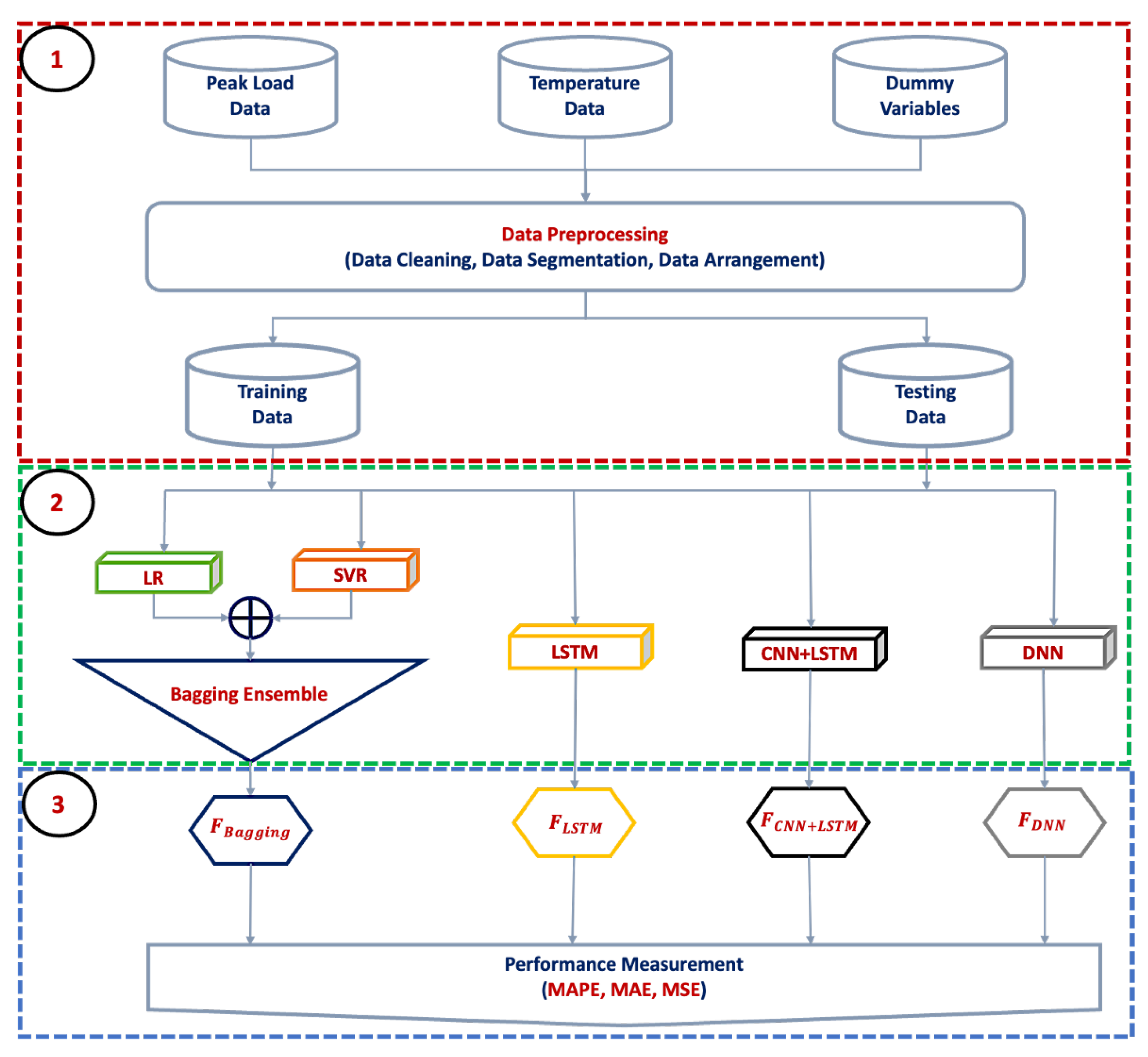
• Bagging ensemble consisting of LR and SVR is firstly proposed to improve the forecasting accuracy by converting ML models from weak learners to strong learners.
• Advanced DL models including DNN, LSTM, and CNN-LSTM are implemented along with tuning hyperparameters for STLF to handle back-propagation learning and time series problems.
• A detailed comparative analysis of the proposed model and other DL models is provided and compared each other. The comparison is done by considering the mean absolute percentage error (MAPE), the mean absolute error (MAE), and the mean squared error (MSE) as the main performance metrics. These performance metrics are computed for the provided dataset for every month.
• The used data in this work are obtained from EGAT and are first smoothed using the filtering technique. The filtering process is done to avoid missing values and outliers.
• Different input features are applied for all models and are compared to check the correlation between load and external influential factors, because external factors like temperature, holidays, and months of the year commonly affect load demand.

1.3. Paper Organization

The rest of the paper is structured using the following sections. Section 2 highlights a brief explanation of the proposed model. This section also includes the framework of the integrated forecasting system. Section 3 discusses and presents the results for the proposed model and compares it with three DL baseline models. Finally, the last section concludes the work.

2. Methodology

This section mainly highlights the framework of the integrated system with key parameters. The readers are encouraged to review the DNN, LSTM, CNN-LSTM and LR models from [11,12,36], as we adopted the theory of these models from the cited works. Figure 1 demonstrates the framework of the proposed models used for forecasting. The integrated system consists of three main parts, named (1) data pre-processing module, (2) training module, and (3) forecasting module. A detailed explanation of each part is revealed in the subsequent subsections.

2.1. Data Pre-Processing Module

The Electricity Generating Authority of Thailand (EGAT) collects the load data from five different regions, which includes the Central area, Bangkok, South, North, and North-East regions in Thailand. The collected load data have been recorded every 30 min from 2009 to 2021. In this paper, the net peak load for the whole country from 2019 to 2021 is applied to test our prediction models. As indicated in Figure 2 and Figure 3, the variations in peak loads react time to time and day to day so that our load data are time series seasonal variation repeating regularly over time. A better insight into the seasonal component in the time series load data could also improve the performance of ML modeling. Consequently, the historical data from the previous week, previous day and previous time are chosen to train the forecasting models. Moreover, temperature data are used as an input because it is one of the external factors affecting loads associated with the meteorological situation in Thailand. The data pre-processing module is further divided into three processes: data cleaning, data segmentation, and data arrangement.

2.1.1. Data Cleaning

The historical data need to be smoothed because there are many missing values and outliers in the original raw data. If these outliers are included in the training data, the accuracy performance of the load predictions would be lower. One additional issue is the normalizing of data. So, it cannot predict the load correctly if the load is higher than previous data. To filter and smooth the raw data, a local regression filtering technique is used. It can be classified into four types: (1) the locally weighted scatterplot smoothing (lowess) regression which uses the method of linear regression analysis, (2) the locally estimated scatterplot smoothing (loess) regression which uses the method of polynomial square regression analysis, (3) robust lowess local regression, and (4) robust loess local regression, which are the robust functions that can be used to get rid of outlier values. If outliers are present in the dataset, load demand fluctuations can cause a reduction in forecasting accuracy. Therefore, a robust lowess/loess (rlowess, rloess) procedure is used to overcome the problem of distorted values of electricity data [37,38]. The loess local regression filtering technique is applied for cleaning data in this experimentation.

The filtering technique fits a local regression function to the data within a chosen neighborhood of data points. A chosen neighborhood is specified by the percentage of data points which is known as a smoothing parameter (0 < smooth ≤ 1). The larger the smoothing parameter, the smoother the graphed function. For calculating smoothed values, this filtering technique specifies a weight for every data point in the selected window by using the regression weight function, as shown in the following equation. Once the regression function values are calculated with flexible weights and polynomial degrees, the rloess fit is complete.

$$w_i={\left(1-{\left|\frac{x-x_i}{d\left(x\right)}\right|}^3\right)}^3.$$

(1)

Equation (1) indicates that x is the predictor value associated with the response value to be smoothed, $w_i$ is the regression weight of points i, $x_i$ is the nearest neighbors of x as defined by the selected window, and $d\left(x\right)$ is the distance along the abscissa from x to the most distant predictor value within the selected window. The data at each period are separated into seven groups based on the day of the week. Therefore, data are cleaned $48\times 7$ times for each period of each day using the rloess function. For example, Monday at 11 am in 2019 and 2021 is smoothed using the filtering technique which is shown in Figure 4. Once the data are filtered, the MiniMax Scaler function, as proposed in the models, is used for normalizing.

2.1.2. Data Segmentation

In all proposed forecasting models, the dataset is divided into training and testing datasets. Each dataset is arranged into seven segments based on the day of the week. For instance, the training dataset consisting of Monday’s load can only forecast the load for Monday. There are 104 data points for the training dataset and 53 pairs for testing in 2021. The proposed models use 104 whole training datasets to test the first Monday of 2021. Then, the data slides to the next 104 training datasets to test another day and perform the same procedure until the end of the testing dataset. This is called “walk-forward”, as shown in Figure 5. The training dataset from 2019–2020 is applied to train both the proposed ensemble and DL models. The empirical results are compared between the bagging ensemble and three DL models.

2.1.3. Selection of Input Features

For the input selection and better data understanding, the Spearman’s correlation coefficient ($\gamma$) was determined to catch nonlinear monotonic correlation between two variables. Figure 6 represents the correlation among all input variables, by showing a value between −1 and +1. A negative $\gamma$ refers to negative correlation, while a positive one is positively correlated. There is no correlation between the two variables if the correlation coefficient is zero. Concerning the correlation illustration, target peak load ($L(t,d)$) positively correlates with $L(t,d-7)$, $L(t,d-1)$, $L(t-2,d-1)$, $L(t-1,d-1)$, $T(t,d-1)$, $SI$ and vice versa. It is slightly negatively correlated with $MoY$, $DoW$, and H, whereas there is a close to zero correlation with $BH$. According to the correlation coefficient, we consider historical peak load and temperature data as main inputs, while other seasonal variables are used as dummy variables. The formula of Spearman’s rank correlation coefficient ($\gamma$) is expressed as below:

$$\gamma =1-(6\sum D_i^2)/N(N^2-1)$$

(2)

where $D_i$ is the difference between the two ranks of each observation and N is the number of observations.

Both the bagging ensemble model and all DL models consist of four different input features, including five, six, nine, and ten input features. Temperature is not included for five and nine forecasting input features. However, a temperature associated with meteorological situations is included in forecasting features of six and ten input features. Other features are dependent on calendar effects, such as day of the week (DoW), month of the year (MoY), holiday (H), and bridging holiday (BH). Forecasting input features are represented by the following equations (Equations (3)–(6)),

For five input features,

$$F_{\left(t,d\right)}=\left[L_{\left(t,d-7\right)},L_{\left(t-2,d-1\right)},L_{\left(t-1,d-1\right)},L_{\left(t,d-1\right)},SI\right]$$

(3)

For six input features,

$$F_{\left(t,d\right)}=\left[L_{\left(t,d-7\right)},L_{\left(t-2,d-1\right)},L_{\left(t-1,d-1\right)},L_{\left(t,d-1\right)},T_{\left(t,d-1\right)},SI\right]$$

(4)

For nine input features,

$$F_{\left(t,d\right)}=\left[L_{\left(t,d-7\right)},L_{\left(t-2,d-1\right)},L_{\left(t-1,d-1\right)},L_{\left(t,d-1\right)},SI,DoW,MoY,H,BH\right]$$

(5)

For ten input features,

$$F_{\left(t,d\right)}=\left[L_{\left(t,d-7\right)},L_{\left(t-2,d-1\right)},L_{\left(t-1,d-1\right)},L_{\left(t,d-1\right)},T_{\left(t,d-1\right)},SI,DoW,MoY,H,BH\right]$$

(6)

where,

$F_{(t,d)}=$ the forecasting vector for input features at time $\left(t\right)$ on the day $\left(d\right)$,

$L_{(t,d-7)}=$ load demand at time t from the previous week $(d-7)$,

$L_{(t-2,d-1)}=$ load demand at two periods before $(t-2)$ on yesterday $(d-1)$,

$L_{(t-1,d-1)}=$ load demand at one period before $(t-1)$ on yesterday $(d-1)$,

$L_{(t,d-1)}=$ load demand at a time $\left(t\right)$ on yesterday $(d-1)$,

$T_{(t,d-1)}=$ temperature at time $\left(t\right)$ on yesterday $(d-1)$,

$SI=$ monthly seasonal index = monthly load/yearly load,

$DoW=$ day of week (Mon = 1, Tue = 2, …, Sun = 7),

$MoY=$ month of year (Jan = 1, Feb = 2, …, Dec =12),

$H=$ holiday (0 or 1) (only holiday is 1, others are 0),

$BH=$ bridging holiday (0 or 1) (only bridging holiday is 1, others are 0).

The example of data arrangement with five inputs for all models is shown in

Table 1. Same day training data arrangement for testing target 1 January 2021 at time t.

Inputs							Target
	No.	${\mathit{L}}_{(\mathit{t},\mathit{d}-\mathit{7})}$	${\mathit{L}}_{(\mathit{t}-\mathit{2},\mathit{d}-\mathbf{1})}$	${\mathit{L}}_{(\mathit{t}-\mathbf{1},\mathit{d}-\mathbf{1})}$	${\mathit{L}}_{(\mathit{t},\mathit{d}-\mathbf{1})}$	$\mathit{SI}$	${\mathit{F}}_{(\mathit{t},\mathit{d})}$
Training Dataset	1	04/01/19 (Fri)	10/01/19 (Thur)	10/01/19 (Thur)	10/01/19 (Thur)	0.98	11/01/19 (Fri)
	.	.	.	.	.	.	.
	.	.	.	.	.	.	.
	.	.	.	.	.	.	.
	104	11/12/20 (Fri)	17/12/20 (Thur)	17/12/20 (Thur)	17/12/20 (Thur)	0.99	18/12/20 (Fri)
Inputs							Target
	No.	${\mathit{L}}_{(\mathit{t},\mathit{d}-\mathbf{7})}$	${\mathit{L}}_{(\mathit{t}-\mathbf{2},\mathit{d}-\mathbf{1})}$	${\mathit{L}}_{(\mathit{t}-\mathbf{1},\mathit{d}-\mathbf{1})}$	${\mathit{L}}_{(\mathit{t},\mathit{d}-\mathbf{1})}$	$\mathit{SI}$	${\mathit{F}}_{(\mathit{t},\mathit{d})}$
Testing Dataset	1	25/12/20 (Fri)	31/12/20 (Thur)	31/12/20 (Thur)	31/12/20 (Thur)	1.02	01/01/21 (Fri)

. According to Table 1, there are five input features to train and test the forecasting models. For training, the dataset from 2019 to 2020 is used and for testing, the dataset from January 2021 to December 2021 is applied.

2.2. Training Module

After arranging the train set and test set based on different input features, the train set is provided into the respective trained model.

2.2.1. Bagging Ensemble Training Process

The bagging ensemble combines LR and SVR models. For the LR training process, M5 prime is used as an expert parameter which indicates the feature selection method to be used during the regression. Additionally, the value is set to 0.05 for min tolerance to eliminate co-linear features during training of the algorithm. For the SVR training process, the model is updated by using stochastic gradient descent (SGD) before updating parameters at every step, converging to a global minimum much faster than ordinary gradient descent. Moreover, the squared error for loss function, 0.0001 alpha learning rate, and one thousand iterations are also tuned in the SVR model.

2.2.2. LSTM Training Process

During training of the LSTM model, the train set and test set are normalized to rescale the original value of the feature between 0 and 1, using the MinMax Scaler function and then fed into the model. The method for normalizing the data is indicated in Equation (7), where $x_i$, $min\left(x\right)$, $max\left(x\right)$, and new $x_i$ represent the original value of the input feature, the minimum value in input feature, the maximum value in input feature, and the new rescaled value of $x_i$.

$$new{x}_i=\frac{x_i-min\left(x\right)}{max\left(x\right)-min\left(x\right)}$$

(7)

The following parameters are selected for fitting the LSTM training process: 100 epochs used for the number of iterations, and mean squared error used as a loss function during the training process. The Adam optimizer is employed over the classical stochastic gradient descent procedure to update network weights iteratively based on training data. In addition, 256 batch sizes are used to work through before updating the internal model parameters. The rectified linear unit (ReLU) is also chosen for the activation function to solve vanishing problems. This activation function can learn much faster than the sigmoid function in networks with many layers, by allowing the training of deeply supervised networks without unsupervised pretraining.

The sequence length of the LSTM network is one of the parameters which have to be considered to train sequential data. EGAT data are recorded by time series every 30 min in one day, so that the data have 48 periods in total. As a consequence, 48 lag features of the load data are used to forecast time steps for the next day. Figure 7 portrays the input feature vectors x, the number of hidden units h, and the output of the final time step o.

2.2.3. CNN-LSTM Training Process

Similar to LSTM, the hybrid CNN-LSTM also uses 100 epochs, 256 batch sizes, an Adam optimizer and ReLU activation function for fitting the model. However, this hybrid model combines two different Dl models: CNN and LSTM so that the data are required to reshape as a subsequence format. Firstly, one dimentional CNN is build with 64 filters, one kernel size and ReLU function, follwed by a maximum pooling layer with two pool sizes and another flattening layer. The next layer is LSTM with 50 networks and ReLU function to execute the final predictions.

2.2.4. DNN Training Process

The DNN model is also well-known as multilayer perceptron (MLP). During the DNN training process, 100 hidden layers and 100 hidden nodes are trained in the network. Other parameters, including 100 epochs, mean squared error for the loss function, Adam optimizer, ReLU for an activation function, are also selected to train the DNN model.

2.3. Forecasting Module

Test data in 2021 are predicted according to the associated trained model. Forecasting performance on the test data is measured using an accuracy measurement. In this study, the mean absolute percentage error (MAPE), the mean absolute error (MAE), and the mean squared error (MSE) in Equations (8)–(10) are regarded as the accuracy measurements which represent how many units of the forecasting value deviate from the actual demand value to calculate an error.

$$MAPE=\frac{1}{t}\sum _{t=1}^{48}\left|\frac{L_t\left(d\right)-F_t\left(d\right)}{L_t\left(d\right)}\right|\times 100\%$$

(8)

$$MAE=\frac{1}{t}\sum _{t=1}^{48}\left|L_t\left(d\right)-F_t\left(d\right)\right|$$

(9)

$$MSE=\frac{1}{t}\sum _{t=1}^{48}{(L_t\left(d\right)-F_t\left(d\right))}^2$$

(10)

where $L_t\left(d\right)$ denotes the actual load on day t and $F_t\left(d\right)$ is the forecasted load on day t.

3. Results and Discussions

The proposed models are evaluated on a MacBook having specifications of an intel Core i5 1.8 GHz processor, 8 GB 1600 MHz DDR3 RAM, and Intel HD graphics 6000 1536 MB, fully loaded with Anaconda navigator and Spyder V3.28 Python Language programming. The Spyder programming has been installed with Tensorflow and Keras libraries. For each data segment, the computation time is set to 10 min.

Table 2. Error Measurements of Test Data for Five Input Features in 2021.

	LSTM			CNN+LSTM			DNN			Bagging Ensemble Model
	MAPE (%)	MAE (MW)	MSE (GW${}^2$)	MAPE (%)	MAE (MW)	MSE (GW${}^2$)	MAPE (%)	MAE (MW)	MSE (GW${}^2$)	MAPE (%)	MAE (MW)	MSE (GW${}^2$)
Jan	13.08	2235.17	9070.42	12.88	2185.09	8397.09	13.72	2359.98	9774.87	12.98	2093.38	8930.46
Feb	4.84	1032.30	1496.87	4.73	1013.17	1579.03	4.76	1014.28	1456.72	3.29	680.38	813.99
Mar	5.97	1445.93	2734.75	6.58	1594.10	3330.44	6.09	1472.09	2827.14	6.48	1569.43	2960.72
Apr	12.68	2652.65	11,081.15	13.12	2746.25	11,586.12	12.71	2663.27	11,132.87	9.94	2130.98	7068.72
May	7.46	1747.65	4822.34	7.14	1664.28	4675.03	7.34	1728.00	4822.21	7.33	1756.00	4480.45
Jun	4.92	1174.47	2056.87	5.14	1227.47	2269.68	4.95	1181.06	2106.70	4.88	1180.28	1970.48
Jul	5.22	1128.93	2049.82	5.12	1111.66	1994.53	5.08	1099.24	1980.59	4.17	907.72	1406.96
Aug	5.35	1201.36	2214.92	5.25	1179.41	2120.09	5.34	1197.99	2212.39	4.17	928.65	1246.86
Sep	3.43	755.24	930.58	4.05	893.08	1239.53	3.40	748.40	905.92	2.36	512.57	421.70
Oct	4.47	977.75	1439.40	4.54	996.56	1455.05	4.59	1004.31	1503.78	3.16	681.71	754.51
Nov	4.74	1040.95	1422.87	4.92	1082.02	1569.09	4.85	1065.46	1478.61	3.88	844.52	928.57
Dec	8.49	1534.56	5032.24	8.51	1545.56	5016.54	8.39	1518.97	4857.91	9.62	1754.26	5920.08
Average	6.74	1413.74	3712.15	6.85	1439.48	3783.01	6.79	1424.50	3772.21	6.05	1258.98	3099.11

presents the error measurements for the discussed parameters (MAPE, MAE, and MSE) for the bagging ensemble and DL baseline models. These parameters are computed and compared monthly while keeping in view five distinct input features. In general, the proposed model provides lower errors than other training models. According to the results provided in Table 2, the proposed bagging model attains a forecasting accuracy of 6.05% in the case of the MAPE parameter. In contrast, the accuracy for LSTM, CNN+LSTM, and DNN are 6.74%, 6.85%, and 6.79%, respectively. This shows that the proposed model outperforms all other training models for the MAPE measurement. A similar trend could also be observed for other parameters. Considering the MAE parameter, the bagging ensemble achieves 1258.98 MW, followed by LSTM with 1413.74 MW, and DNN with 1424.50 MW. The least performance is shown by the CNN+LSTM model, contributing to 1439.48 MW. Similar behavior is observed for the MSE parameter, where bagging realizes 3099.11 GW${}^2$. After the proposedmodel, LSTM performs better with 3712.15 GW${}^2$. Finally, the MSEs of the DNN and CNN+LSTM models are 3783.01 GW${}^2$ and 3772.21 GW${}^2$, respectively. Although the proposed ensemble gives better performance, January, April, May, and December still get higher errors in all models because these months have long holidays and tourism seasons. Another factor is the highest temperature in April and May. Hence, electricity consumption is higher than usual. In contrast, the proposed model observed the lowest MAPE, showing 2.36% MAPE, 512.57 MW MAE, and 421.70 GW${}^2$ MSE in September. Next, the DNN model performs well, followed by LSTM and CNN+LSTM models.

Table 3. Error Measurements of Test Data for Six Input Features in 2021.

	LSTM			CNN+LSTM			DNN			Bagging Ensemble Model
	MAPE (%)	MAE (MW)	MSE (GW${}^2$)	MAPE (%)	MAE (MW)	MSE (GW${}^2$)	MAPE (%)	MAE (MW)	MSE (GW${}^2$)	MAPE (%)	MAE (MW)	MSE (GW${}^2$)
Jan	13.47	2302.89	9434.34	12.82	2169.25	8326.74	13.66	2346.44	9702.55	13.30	2156.66	9328.55
Feb	4.94	1052.54	1555.61	4.71	1008.24	1569.31	4.74	1010.59	1445.70	4.08	849.31	1041.12
Mar	5.64	1363.73	2474.69	6.57	1592.86	3317.03	6.05	1463.81	2793.74	6.17	1491.13	2771.64
Apr	12.85	2685.20	11,407.45	13.09	2737.26	11,567.10	12.68	2655.50	11,063.96	9.36	2017.90	6383.87
May	7.38	1730.76	4733.29	7.15	1666.79	4664.40	7.33	1725.31	4803.78	7.60	1818.32	4736.45
Jun	4.86	1156.05	2005.84	5.13	1225.57	2254.33	4.94	1180.03	2092.43	4.79	1155.41	1900.14
Jul	5.40	1165.50	2172.26	5.11	1108.74	1985.82	5.07	1097.75	1973.20	4.30	933.69	1472.71
Aug	5.22	1169.25	2168.62	5.23	1175.00	2109.25	5.33	1197.39	2206.47	4.09	911.47	1195.68
Sep	3.34	731.34	859.70	4.04	891.51	1233.88	3.38	744.35	898.31	2.44	529.81	462.55
Oct	4.40	958.21	1431.91	4.53	995.41	1452.99	4.57	1001.54	1500.10	3.28	711.41	794.38
Nov	4.64	1014.20	1358.34	4.92	1081.30	1565.14	4.85	1066.07	1476.86	3.91	855.13	903.18
Dec	8.68	1568.35	5228.79	8.50	1542.71	5014.64	8.36	1513.71	4840.41	9.33	1699.77	5656.51
Average	6.75	1411.22	3751.94	6.83	1435.82	3768.63	6.77	1420.27	3750.29	6.08	1265.55	3077.47

also indicates error measurements for all models, training with six input features. Similar to Table 2, the best forecasting accuracy is realized by the proposed model, at 6.08% MAPE, 1265.55 MW MAE, and 3077.47 GW${}^2$ MSE. The second model is the LSTM model, providing 6.75% MAPE, 1411.22 MW MAE, and 3751.94 GW${}^2$ MSE, as opposed to the DNN model with 6.77% MAPE, 1420.27 MW MAE, and 3750.29 GW${}^2$ MSE. The hybrid CNN and LSTM model demonstrates the least forecasting accuracy with 6.83% MAPE, 1435.82 MW MAE, and 3768.83 GW${}^2$ MSE. For the holiday season, there is not much error difference on including temperature as an input feature in the training models.

Monthly error accuracies for all models using nine inputs that have additional dummy variables in terms of calendar effects are measured in

Table 4. Error Measurements of Test Data for Nine Input Features in 2021.

	LSTM			CNN+LSTM			DNN			Bagging Ensemble Model
	MAPE (%)	MAE (MW)	MSE (GW${}^2$)	MAPE (%)	MAE (MW)	MSE (GW${}^2$)	MAPE (%)	MAE (MW)	MSE (GW${}^2$)	MAPE (%)	MAE (MW)	MSE (GW${}^2$)
Jan	13.86	2365.26	10,111.87	13.29	2269.25	9485.31	13.65	2344.11	9724.30	15.34	2564.18	10,180.74
Feb	4.87	1034.95	1515.81	4.65	995.74	1534.25	4.71	1003.79	1427.19	5.88	1213.62	2052.17
Mar	5.43	1311.84	2321.53	6.49	1572.13	3250.22	5.98	1445.96	2745.80	4.01	982.23	1392.94
Apr	12.95	2698.69	11,588.90	13.15	2749.12	11,644.37	12.74	2667.98	11,151.51	7.93	1735.60	4007.19
May	7.42	1739.76	4787.04	7.18	1671.46	4699.33	7.33	1724.78	4804.21	7.00	1663.69	4013.99
Jun	4.87	1156.13	2067.77	5.14	1229.19	2272.48	4.94	1180.86	2102.16	4.72	1141.76	1934.57
Jul	5.63	1215.65	2372.88	5.13	1114.11	2005.08	5.09	1101.11	1989.94	3.68	812.37	1050.80
Aug	5.17	1155.53	2170.30	5.26	1182.95	2129.16	5.35	1201.38	2225.85	4.33	967.23	1347.89
Sep	3.35	733.56	878.89	4.09	903.07	1259.64	3.40	749.55	909.87	2.39	522.24	441.59
Oct	4.45	966.99	1479.57	4.57	1004.25	1472.86	4.61	1009.43	1514.38	4.13	907.69	1252.86
Nov	4.67	1021.29	1381.03	4.95	1088.48	1585.90	4.88	1073.17	1499.20	4.13	915.09	1122.71
Dec	8.86	1597.99	5527.36	8.50	1544.94	4965.67	8.36	1513.95	4818.58	7.22	1317.83	3443.50
Average	6.82	1419.76	3868.02	6.89	1446.87	3874.16	6.77	1421.41	3759.89	5.91	1230.39	2700.84

. In this case, the bagging ensemble model outperforms all other discussed training models, showing 5.91% MAPE, 1230.39 MW MAE, and 2700.84 GW${}^2$ MSE. Regarding the average accuracy, the DNN model attains 6.77% MAPE, 1421.41 MW MAPE, and 3759.89 GW${}^2$ MSE, while the LSTM and CNN+LSTM models observe 0.1% lower MAPE than the DNN model. In this case, adding dummy variables slightly increases the forecasting accuracy of our bagging ensemble model.

As illustrated in

Table 5. Error Measurements of Test Data for Ten Input Features in 2021.

	LSTM			CNN+LSTM			DNN			Bagging Ensemble Model
	MAPE (%)	MAE (MW)	MSE (GW${}^2$)	MAPE (%)	MAE (MW)	MSE (GW${}^2$)	MAPE (%)	MAE (MW)	MSE (GW${}^2$)	MAPE (%)	MAE (MW)	MSE (GW${}^2$)
Jan	13.06	2222.83	9319.77	13.31	2278.28	9906.45	13.61	2336.18	9664.02	10.71	1771.09	5929.37
Feb	4.60	977.39	1362.42	4.73	1012.83	1575.91	4.70	1001.53	1421.40	4.39	905.93	1309.20
Mar	5.28	1276.51	2283.40	6.60	1600.12	3342.88	5.98	1445.98	2741.79	4.01	993.48	1511.03
Apr	13.49	2847.43	12,129.30	13.07	2733.13	11,532.10	12.70	2659.44	11,102.30	9.97	2142.93	6530.93
May	7.17	1677.72	4506.97	7.16	1669.31	4681.90	7.32	1723.51	4796.36	7.10	1677.81	4510.27
Jun	4.93	1170.28	2077.95	5.11	1222.13	2246.29	4.93	1177.09	2088.14	4.75	1138.79	2089.53
Jul	5.67	1222.75	2355.99	5.10	1107.68	1979.51	5.08	1100.32	1984.25	4.97	1073.62	1766.54
Aug	5.32	1190.37	2223.38	5.22	1173.59	2104.87	5.33	1196.94	2210.42	5.48	1232.26	2356.22
Sep	3.34	729.84	858.84	4.04	890.43	1232.04	3.39	747.37	904.26	3.33	731.15	882.58
Oct	4.42	959.36	1463.77	4.53	994.94	1451.84	4.60	1007.93	1511.07	4.85	1070.56	1878.72
Nov	4.70	1026.40	1402.03	4.90	1078.62	1559.26	4.87	1069.95	1490.00	4.40	973.18	1313.48
Dec	8.82	1590.31	5466.79	8.50	1542.88	5013.12	8.34	1511.40	4813.56	7.79	1423.98	3846.71
Average	6.75	1410.74	3803.87	6.87	1445.09	3901.68	6.76	1418.22	3744.40	6.00	1264.31	2840.87

, ten inputs, including additional temperature and dummy variables, are trained for all models to measure the accuracy. In this case, our proposed model still provides the minimum error with 6.00% MAPE, 1264.31 MW MAE, and 2840.87 GW${}^2$ MSE. The LSTM and DNN came next with almost similar MAPE, representing around 6.75% MAPE, followed by the CNN+LSTM model having 6.87% MAPE. According to all four result tables (Table 2, Table 3, Table 4 and Table 5), our proposed model has no sensitivity for the selection of input features because of similar resulting errors. However, additional temperature input only causes a higher error in the proposed model. Each forecasting model obtains the minimum error on different input features in the comparative analysis among input features. The LSTM, CNN-LSTM, DNN models correspondingly provide the lowest error at five inputs, six inputs, and ten inputs. All in all, our proposed model executes the best performance in all experiments.

Five categories, such as holidays, bridging holidays, Mondays, weekdays, and weekends are grouped for all four forecasting models to check the MAPE results in each category.

Table 6. Average MAPE for Five Categories with Different Input Features in Percent.

	Five Inputs				Six Inputs				Nine Inputs				Ten Inputs
	LSTM	CNN+LSTM	DNN	Bagging Ensemble Model	LSTM	CNN+LSTM	DNN	Bagging Ensemble Model	LSTM	CNN+LSTM	DNN	Bagging Ensemble Model	LSTM	CNN+LSTM	DNN	Bagging Ensemble Model
Holidays	20.19	20.23	20.09	18.78	20.29	20.29	20.08	19.01	20.77	20.30	20.07	15.60	20.45	20.25	20.07	16.10
Bridging Holidays	9.5	10.16	9.26	7.76	10.07	10.28	9.25	8.16	10.49	10.22	9.26	6.56	10.07	10.20	9.25	8.41
Mondays	5.39	5.39	5.42	5.73	5.39	5.39	5.42	5.73	5.47	5.35	5.44	5.80	5.35	5.39	5.42	5.17
Weekdays	5.6	5.79	5.63	4.92	5.62	5.76	5.60	4.93	5.61	5.84	5.61	4.80	5.64	5.86	5.59	5.00
Weekends	6.64	6.67	6.78	5.66	6.62	6.64	6.76	5.68	6.71	6.70	6.77	6.02	6.56	6.61	6.75	6.10

refers to the average MAPE of 2021 test predictions for all models according to different input structures. Overall, holidays have influenced MAPE values immensely, providing a higher range of values irrespective of the input features. The proposed model’s holiday category offers around 2% to 4% lower than other models in all forecasting structures. Similarly, other models provide inferior performance to the proposed model in the group of bridging holidays. The category of Mondays shows the minimum influence in all DL models. Nevertheless, the proposed model has a worse performance than others in all features, except ten inputs having minimum MAPE. Regarding the group of weekdays and weekends, the bagging ensemble performs similar error percentages in all input features, varying approximately 5% to 6%, while other models range from 6% to 7%. Over and above, the proposed model outperforms other baseline models (LSTM, CNN+LSTM, and DNN) in all categories, except the group of Mondays.

4. Conclusions

In this paper, the ML-based bagging ensemble model combining LR and SVR was proposed. Moreover, three advanced DL models, i.e., LSTM, CNN+LSTM, and DNN models were implemented as benchmark models for forecasting comparative analysis. The collected data were gathered from the Electricity Generating Authority of Thailand (EGAT). All models were trained and tested by using cleaned data from 2019 to 2020 to forecast daily load demand in 2021. The proposed and benchmark models were trained on both without temperature using five and nine input features, and with temperature using six and ten input features. The nine and ten input features include dummy features based on the calendar. Feature selection did not have much effect on any of the forecasting models as it executes almost stable errors for all features. However, the temperature input did not help to improve the accuracy. In addition, results were compared using five different categories (holidays, bridging holidays, Mondays, weekdays, and weekends). The proposed model provides a better performance than other models in all categories, except in the category of Mondays. To sum up, apart from our proposed model, each forecasting model is good at different features by giving reasonable accuracies. This result in our proposed model could improve performance and each model could handle the sensitivity of feature variance in forecasting.

References

1. Andriopoulos, N.; Magklaras, A.; Birbas, A.; Papalexopoulos, A.; Valouxis, C.; Daskalaki, S.; Birbas, M.; Housos, E.; Papaioannou, G.P. Short Term Electric Load Forecasting Based on Data Transformation and Statistical Machine Learning. Appl. Sci. 2021, 11, 158. [Google Scholar] [CrossRef]
2. Papalexopoulos, A.D.; Hesterberg, T.C. A regression-based approach to short-term system load forecasting. IEEE Trans. Power Syst. 1990, 5, 1535–1547. [Google Scholar] [CrossRef]
3. Henselmeyer, S.; Grzegorzek, M. Short-Term Load Forecasting Using an Attended Sequential Encoder-Stacked Decoder Model with Online Training. Appl. Sci. 2021, 11, 4927. [Google Scholar] [CrossRef]
4. Christiaanse, W. Short-term load forecasting using general exponential smoothing. IEEE Trans. Power Appar. Syst. 1971, PAS-90, 900–911. [Google Scholar] [CrossRef]
5. Liu, K.; Subbarayan, S.; Shoults, R.; Manry, M.; Kwan, C.; Lewis, F.; Naccarino, J. Comparison of very short-term load forecasting techniques. IEEE Trans. Power Syst. 1996, 11, 877–882. [Google Scholar] [CrossRef]
6. Mohandes, M. Support vector machines for short-term electrical load forecasting. Int. J. Energy Res. 2002, 26, 335–345. [Google Scholar] [CrossRef]
7. Hippert, H.S.; Pedreira, C.E.; Souza, R.C. Neural networks for short-term load forecasting: A review and evaluation. IEEE Trans. Power Syst. 2001, 16, 44–55. [Google Scholar] [CrossRef]
8. Azadeh, A.; Saberi, M.; Gitiforouz, A. An integrated simulation-based fuzzy regression-time series algorithm for electricity consumption estimation with non-stationary data. J. Chin. Inst. Eng. 2011, 34, 1047–1066. [Google Scholar] [CrossRef]
9. Sapankevych, N.I.; Sankar, R. Time series prediction using support vector machines: A survey. IEEE Comput. Intell. Mag. 2009, 4, 24–38. [Google Scholar] [CrossRef]
10. Bottou, L. Large-scale machine learning with stochastic gradient descent. In Proceedings of the COMPSTAT’2010, Paris, France, 22–27 August 2010; pp. 177–186. [Google Scholar]
11. Saber, A.Y.; Alam, A.R. Short term load forecasting using multiple linear regression for big data. In Proceedings of the 2017 IEEE Symposium Series on Computational Intelligence (SSCI), Honolulu, HI, USA, 27 November–1 December 2017; pp. 1–6. [Google Scholar]
12. Phyo, P.P.; Jeenanunta, C.; Hashimoto, K. Electricity load forecasting in Thailand using deep learning models. Int. J. Electr. Electron. Eng. Telecommun. 2019, 8, 221–225. [Google Scholar] [CrossRef]
13. Hinton, G.E.; Osindero, S.; Teh, Y.W. A fast learning algorithm for deep belief nets. Neural Comput. 2006, 18, 1527–1554. [Google Scholar] [CrossRef] [PubMed]
14. Li, H.; Deng, J.; Yuan, S.; Feng, P.; Arachchige, D.D. Monitoring and Identifying Wind Turbine Generator Bearing Faults Using Deep Belief Network and EWMA Control Charts. Front. Energy Res. 2021, 9, 799039. [Google Scholar] [CrossRef]
15. Hochreiter, S.; Schmidhuber, J. Long short-term memory. Neural Comput. 1997, 9, 1735–1780. [Google Scholar] [CrossRef] [PubMed]
16. Urban, G.; Geras, K.J.; Kahou, S.E.; Aslan, O.; Wang, S.; Caruana, R.; Mohamed, A.; Philipose, M.; Richardson, M. Do deep convolutional nets really need to be deep and convolutional? arXiv 2016, arXiv:1603.05691. [Google Scholar]
17. Phyo, P.P.; Byun, Y.C.; Park, N. Short-Term Energy Forecasting Using Machine-Learning-Based Ensemble Voting Regression. Symmetry 2022, 14, 160. [Google Scholar] [CrossRef]
18. Liu, W.; Wang, Z.; Liu, X.; Zeng, N.; Liu, Y.; Alsaadi, F.E. A survey of deep neural network architectures and their applications. Neurocomputing 2017, 234, 11–26. [Google Scholar] [CrossRef]
19. Dedinec, A.; Filiposka, S.; Dedinec, A.; Kocarev, L. Deep belief network based electricity load forecasting: An analysis of Macedonian case. Energy 2016, 115, 1688–1700. [Google Scholar] [CrossRef]
20. Phyo, P.P.; Jeenanunta, C. Daily Load Forecasting Based on a Combination of Classification and Regression Tree and Deep Belief Network. IEEE Access 2021, 9, 152226–152242. [Google Scholar] [CrossRef]
21. Qiu, X.; Zhang, L.; Ren, Y.; Suganthan, P.N.; Amaratunga, G. Ensemble deep learning for regression and time series forecasting. In Proceedings of the 2014 IEEE Symposium on Computational Intelligence in Ensemble Learning (CIEL), Orlando, FL, USA, 9–12 December 2014; pp. 1–6. [Google Scholar]
22. El-Sharkh, M.Y.; Rahman, M.A. Forecasting electricity demand using dynamic artificial neural network model. In Proceedings of the 2012 International Conference on Industrial Engineering and Operations Management, Istanbul, Turkey, 3–6 July 2012; pp. 3–6. [Google Scholar]
23. Rashid, T.; Huang, B.; Kechadi, M.; Gleeson, B. Auto-regressive recurrent neural network approach for electricity load forecasting. Int. J. Comput. Intell. 2006, 3, 1–9. [Google Scholar]
24. Hatalis, K.; Pradhan, P.; Kishore, S.; Blum, R.S.; Lamadrid, A.J. Multi-step forecasting of wave power using a nonlinear recurrent neural network. In Proceedings of the 2014 IEEE PES General Meeting|Conference & Exposition, National Harbor, MD, USA, 27–31 July 2014; pp. 1–5. [Google Scholar]
25. Kelo, S.; Dudul, S. A wavelet Elman neural network for short-term electrical load prediction under the influence of temperature. Int. J. Electr. Power Energy Syst. 2012, 43, 1063–1071. [Google Scholar] [CrossRef]
26. Cheng, Y.; Xu, C.; Mashima, D.; Thing, V.L.; Wu, Y. PowerLSTM: Power demand forecasting using long short-term memory neural network. In Proceedings of the International Conference on Advanced Data Mining and Applications, Singapore, 5–6 November 2017; pp. 727–740. [Google Scholar]
27. Bouktif, S.; Fiaz, A.; Ouni, A.; Serhani, M.A. Optimal deep learning lstm model for electric load forecasting using feature selection and genetic algorithm: Comparison with machine learning approaches. Energies 2018, 11, 1636. [Google Scholar] [CrossRef] [Green Version]
28. Syed, D.; Abu-Rub, H.; Ghrayeb, A.; Refaat, S.S. Household-level energy forecasting in smart buildings using a novel hybrid deep learning model. IEEE Access 2021, 9, 33498–33511. [Google Scholar] [CrossRef]
29. Ullah, I.; Liu, K.; Yamamoto, T.; Zahid, M.; Jamal, A. Electric vehicle energy consumption prediction using stacked generalization: An ensemble learning approach. Int. J. Green Energy 2021, 18, 896–909. [Google Scholar] [CrossRef]
30. Khan, A.N.; Iqbal, N.; Ahmad, R.; Kim, D.H. Ensemble prediction approach based on learning to statistical model for efficient building energy consumption management. Symmetry 2021, 13, 405. [Google Scholar] [CrossRef]
31. Dong, Z.; Liu, J.; Liu, B.; Li, K.; Li, X. Hourly energy consumption prediction of an office building based on ensemble learning and energy consumption pattern classification. Energy Build. 2021, 241, 110929. [Google Scholar] [CrossRef]
32. Ngo, N.T.; Pham, A.D.; Truong, T.T.H.; Truong, N.S.; Huynh, N.T.; Pham, T.M. An ensemble machine learning model for enhancing the prediction accuracy of energy consumption in buildings. Arab. J. Sci. Eng. 2022, 47, 4105–4117. [Google Scholar] [CrossRef]
33. Wang, X.; Wang, S.; Zhao, Q.; Wang, S.; Fu, L. A multi-energy load prediction model based on deep multi-task learning and ensemble approach for regional integrated energy systems. Int. J. Electr. Power Energy Syst. 2021, 126, 106583. [Google Scholar]
34. da Silva, R.G.; Ribeiro, M.H.D.M.; Moreno, S.R.; Mariani, V.C.; dos Santos Coelho, L. A novel decomposition-ensemble learning framework for multi-step ahead wind energy forecasting. Energy 2021, 216, 119174. [Google Scholar] [CrossRef]
35. Li, H.; Deng, J.; Feng, P.; Pu, C.; Arachchige, D.D.; Cheng, Q. Short-Term Nacelle Orientation Forecasting Using Bilinear Transformation and ICEEMDAN Framework. Front. Energy Res. 2021, 9, 780928. [Google Scholar] [CrossRef]
36. Phyo, P.P.; Byun, Y.C. Hybrid Ensemble Deep Learning-Based Approach for Time Series Energy Prediction. Symmetry 2021, 13, 1942. [Google Scholar] [CrossRef]
37. Jeenanunta, C.; Abeyrathna, K.D.; Dilhani, M.S.; Hnin, S.W.; Phyo, P.P. Time series outlier detection for short-term electricity load demand forecasting. Int. Sci. J. Eng. Technol. (ISJET) 2018, 2, 37–50. [Google Scholar]
38. Rashid, F.; Ahmad, R.; Talha, H.M.; Khalid, A. Dynamic Load Sharing at Domestic Level Using the Internet of Things. Int. J. Integr. Eng. 2020, 12, 57–65. [Google Scholar] [CrossRef]
Figure 1. Overview of the integrated system for STLF, including 1. data pre-processing module, 2. training module, and 3. forecasting module.
Applsci 12 04882 g001
Figure 2. Variation in peak load based on day of week from 2019 to 2021.
Applsci 12 04882 g002
Figure 3. Variation in peak load based on time of the day (hourly) from 2019 to 2021.
Applsci 12 04882 g003
Figure 4. Relationship between original data and smoothed data.
Applsci 12 04882 g004
Figure 5. Sample dataset for walk-forward testing routine.
Applsci 12 04882 g005
Figure 6. Correlation for all input variables.
Applsci 12 04882 g006
Figure 7. The Sequence Length of LSTM for Electricity Load Data.
Applsci 12 04882 g007