Article

A 3D Fluorescence Classification and Component Prediction Method Based on VGG Convolutional Neural Network and PARAFAC Analysis Method

1
College of Information Engineering, Sichuan Agricultural University, Ya’an 625000, China
2
College of Environmental Sciences, Sichuan Agricultural University, Ya’an 625000, China
3
College of Resources, Sichuan Agricultural University, Chengdu 611130, China
4
College of Science, Sichuan Agricultural University, Ya’an 625000, China
*
Author to whom correspondence should be addressed.
Appl. Sci. 2022, 12(10), 4886; https://doi.org/10.3390/app12104886
Submission received: 7 April 2022 / Revised: 26 April 2022 / Accepted: 9 May 2022 / Published: 12 May 2022
(This article belongs to the Section Environmental Sciences)

Abstract

:
Three-dimensional fluorescence is currently studied by methods such as parallel factor analysis (PARAFAC), fluorescence regional integration (FRI), and principal component analysis (PCA). There are also many studies combining convolutional neural networks at present, but there is no one method recognized as the most effective among the methods combining convolutional neural networks and 3D fluorescence analysis. Based on this, we took some samples from the actual environment for measuring 3D fluorescence data and obtained a batch of public datasets from the internet species. Firstly, we preprocessed the data (including two steps of PARAFAC analysis and CNN dataset generation), and then we proposed a 3D fluorescence classification method and a components fitting method based on VGG16 and VGG11 convolutional neural networks. The VGG16 network is used for the classification of 3D fluorescence data with a training accuracy of 99.6% (as same as the PCA + SVM method (99.6%)). Among the component maps fitting networks, we comprehensively compared the improved LeNet network, the improved AlexNet network, and the improved VGG11 network, and finally selected the improved VGG11 network as the component maps fitting network. In the improved VGG11 network training, we used the MSE loss function and cosine similarity to judge the merit of the model, and the MSE loss of the network training reached 4.6 × 10⁻⁴ (characterizing the variability of the training results and the actual results), and we used the cosine similarity as the accuracy criterion, and the cosine similarity of the training results reached 0.99 (comparison of the training results and the actual results). The network performance is excellent. The experiments demonstrate that the convolutional neural network has a great application in 3D fluorescence analysis.

1. Introduction

The treatment of organic pollution in rivers and drinking water is one of the social problems that needs to be dealt with for the development of human society, and the water pollution situation is related to people’s health and is widely present in natural water bodies [1,2,3]. In recent years, more and more attention has been paid to organic pollution in rivers and drinking water [4], and therefore to water quality monitoring methods [5]. For example, the use of three-dimensional fluorescence and PARAFAC analysis methods to track the treatment of natural organics in drinking water treatment plants [6], combined with three-dimensional fluorescence using open set identification methods to identify organic contamination in water bodies [7]. In addition, there are still many methods that use PCA, SVM, and deep learning algorithms combined with 3D fluorescence for analysis [8,9].
According to previous studies, three-dimensional fluorescence has been widely used in the analysis of water pollution [10] and various foods [11]. Most of these organic substances such as humic acids, lignin, aromatic amino acids, and DNA can be analyzed by fluorescence [12]. When these substances are present in solution and different types and concentrations, their fluorescence characteristics follow the changes. Therefore, three-dimensional fluorescence can be used to distinguish and detect different organic solutions [13,14,15]. In addition, 3D fluorescence differs from 2D fluorescence in that it consists of a large number of excitation–emission fluorescence matrices, so an efficient 3D fluorescence interpretation method is needed to extract useful components information from 3D fluorescence data [16].
There have been many analytical methods for 3D fluorescence. Wenchen et al. used the FRI method for the effective analysis of DOM components [17]. Yamashita Y et al. [18] used PARAFAC analysis to characterize the interactions between trace metals and dissolved organic matter. Ruiyu Xu and others [9] used PCA combined with SVM to classify and identify Chinese strong aroma-type liquors. Francesca Guimet et al. [19] used the expanded principal component analysis combined with PARAFAC analysis to distinguish pure olive oil and virgin olive oil, founding three classes of possible compounds. Ramila H. Peiris et al. [20] used the PCA method to track pollutants in the drinking water treatment process. C. W. cuss et al. [21] used four machine learning algorithms (i.e., decision tree, k-nearest neighbor, multilayer perceptron, and support vector machine) combined with the PARAFAC analysis method to classify a large number of 3D-EEMs data. In addition, there are also many research papers on 3D-EEMs data combined with deep learning algorithms. For example, Shi Fei [7] understood the 3D-EEMs matrix as an image channel, added X and Y coordinate channels, and established an organic pollutants evaluation model based on a position convolution network (CoordConv) and cosine similarity. Wu Xijun [22] used the contour map generated by 3D-EEMs as the training dataset of AlexNet, combined with SVM and PLS (least square method) to judge whether there is forgery in sesame oil, and obtained a 100% recognition accuracy. Xu Runze [8], combined with the analysis results of PARAFAC analysis, predicted the number of components of different kinds of 3D-EEMs data by using the NCNN network (a revolutionary neural network model for the number of fluorescent components) and fitted the components with MCNN network (a revolutionary neural network model for the map of fluorescent components). In addition, Lu Zhiwei [23] used yolo-v3 algorithm to classify and recognize the fluorescent image and used the algorithm to segment the fluorescent region. They analyzed the relationship between heavy metal ions in agricultural residues and fluorescence intensity from the perspective of RGB value, HSV value, and the concentration of agricultural residues. Liu Tao [24] also used the yolo-v3 algorithm combined with the wechat applet to detect and classify fluorescence images and realized a scheme to quickly detect GSH and ADA on site based on an image processing algorithm.
Based on the above research, nowadays, in addition to the traditional FRI, PCA, and PARAFAC, etc., there have been many machine learning algorithms and deep learning algorithms to prove the feasibility of the study of 3D fluorescence data. Based on these studies, combined with the analysis results of PARAFAC analysis and VGG16 and VGG11 convolutional neural network, in this paper, we developed a new 3D fluorescence data classification model and 3D fluorescence component maps fitting model. Among them, VGG16 is used for the classification of 3D fluorescence data, which is used to classify the 3D fluorescence from different sources. VGG11 is used for components map fitting, and compared with the MCNN model of Xu et al., this model does not need to create a submodel for each component map but determines the number of submodels based on the maximum number of components of 3D fluorescence, which makes the components fitting model more robust and prevents the overfitting effect of the network. In addition, VGG11 has a better fitting effect by comparing the model results with AlexNet and LeNet (the backbone network used by MCNN). Experiments show that according to the PARAFAC analysis results, the convolutional neural network can predict the category of 3D fluorescence data and fit its specific components map only by inputting a single 3D fluorescence datum. In this way, we don’t need to perform complex PARAFAC analysis on 3D-EEMs and can quickly obtain the category and components map of 3D fluorescence data using CNN models only, which provides a reliable technical means in river monitoring, drinking water monitoring, and other scenes that need rapid results.

2. Materials and Methods

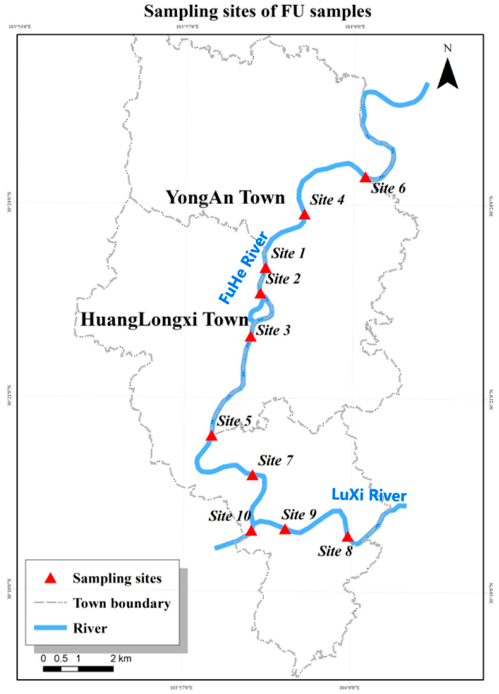
2.1. Samples Collection

We collected 3D fluorescence data from different sources. The first part is 45 3D fluorescence samples (FU) collected from Fu River (the reach of Huanglongxi town and Yong’an town) in Shuangliu District, Chengdu City, China. The second part is the data published in the article (Murphy et al. (2013)) [25] including 206 3D fluorescence samples (P). The third part is the “Pure Tutorial” from drEEM toolbox, including 60 3D fluorescence data samples (PU). The fourth part is 105 3D fluorescence data samples (F) extracted from fish molecules (Andersen et al.) [11]. Despite that the datasets are from different regions and using different raw materials, they all have similar characteristics of 3D fluorescence data. The details of these datasets are shown in Table 1.
The FU dataset contains a total of 45 samples, all of which were collected from the Fu River and its surroundings. A total of 10 sites were collected (samples in site 8 and site 9 were not located in Fu River. For meticulous samples collection sites, please refer to Figure 1). Among them, 10 samples were collected from site 1 and site 10, respectively, 8 samples were collected from site 7, 5 samples were collected from site 2, and 3 samples were collected from site 3, site 4, site 5, and site 6, respectively. The collected river water samples were refrigerated in an incubator at 5 °C, and the measurement shall be completed within 12 h of being kept at a low temperature. Before measuring 3D fluorescence, the samples were filtered using a sterile syringe with a 0.45 μm microporous filter membrane (the syringe and filter membrane and the quartz dish were each repeatedly washed three times with 3 mL of sample solution before filtration). The P dataset was collected from 26 different sites and 4 different cruises. After removing the abnormal samples, the remaining 206 samples were used in this experiment. The PU dataset consists of pure fluorescence from the “Pure Tutorial” in the drEEM V0.6, which contains 60 samples. The F dataset is from frozen cod fillets, which were stored at 2 °C for 21 days. To expand the variation of products, different frozen storage temperatures, frozen storage periods, and refrigerated storage periods were used. Therefore, the 3D fluorescence data come from different periods with some quantitative differences.

2.2. 3D-EEMs Measurement

For the FU dataset, the Hitachi F-4500 fluorescence spectrometer was used to measure its three-dimensional fluorescence data (the concentration of organic matter in the river water is relatively low, in this study, we selected several samples for dilution and repeated measurements to ensure that no fluorescence in-filtering effect occurred in the river water [26]). During the measurement, the excitation wavelength was set to 200–500 nm with an interval of 10 nm; the emission wavelength was set to 250–550 nm with an interval of 5 nm, the excitation and emission slits were both set to 10 nm, the PMT voltage was set to 700 V, and the scanning speed was set to 1200 nm/min. The measurement of F data and P data can be found in published articles (Andersen et al., Murphy et al.), while the PU data are accurately described in the official drEEM toolbox V0.6 documentation.
To use convolutional neural networks for classification and component maps fitting of 3D fluorescence data, the prerequisite is to obtain 3D fluorescence data. During the 3D fluorescence measurement experiment of the FU dataset, in total we measured and obtained 45 samples (except outlier samples), each 3D-EEM consists of 31 excitation spectra and 61 emission spectra, therefore, the 3D-EEM size is 61 × 31.
In the other three types of datasets, the F dataset was measured by fluorescence spectrometry using a Perkin Elmer LS50B fluorescence spectrometer in 10 nm × 10 nm quartz cuvettes with excitation spectra ranging from 250–370 nm with an excitation interval of 10 nm and emission spectra ranging from 270–600 nm with an emission interval of 1 nm. each emission–excitation matrix consists of 13 excitation spectra and 331 emission spectra, and the 3D-EEM size is 331 × 13. In the P dataset, the excitation spectra range from 230–455 nm with an excitation interval of 5 nm, the emission spectra range from 290–682 nm with an emission interval of 4 nm, and each emission–excitation matrix consists of 46 excitation spectra and 99 emission spectra, and the 3D-EEM size is 99 × 46. In the PU dataset, the excitation spectra range from 243–399 nm with an interval of 4 nm, the emission spectra range from 303–499 nm with an emission interval of 4 nm, and each emission-excitation matrix consists of 40 excitation spectra and 50 emission spectra, and the 3D-EEM size is 50 × 40.

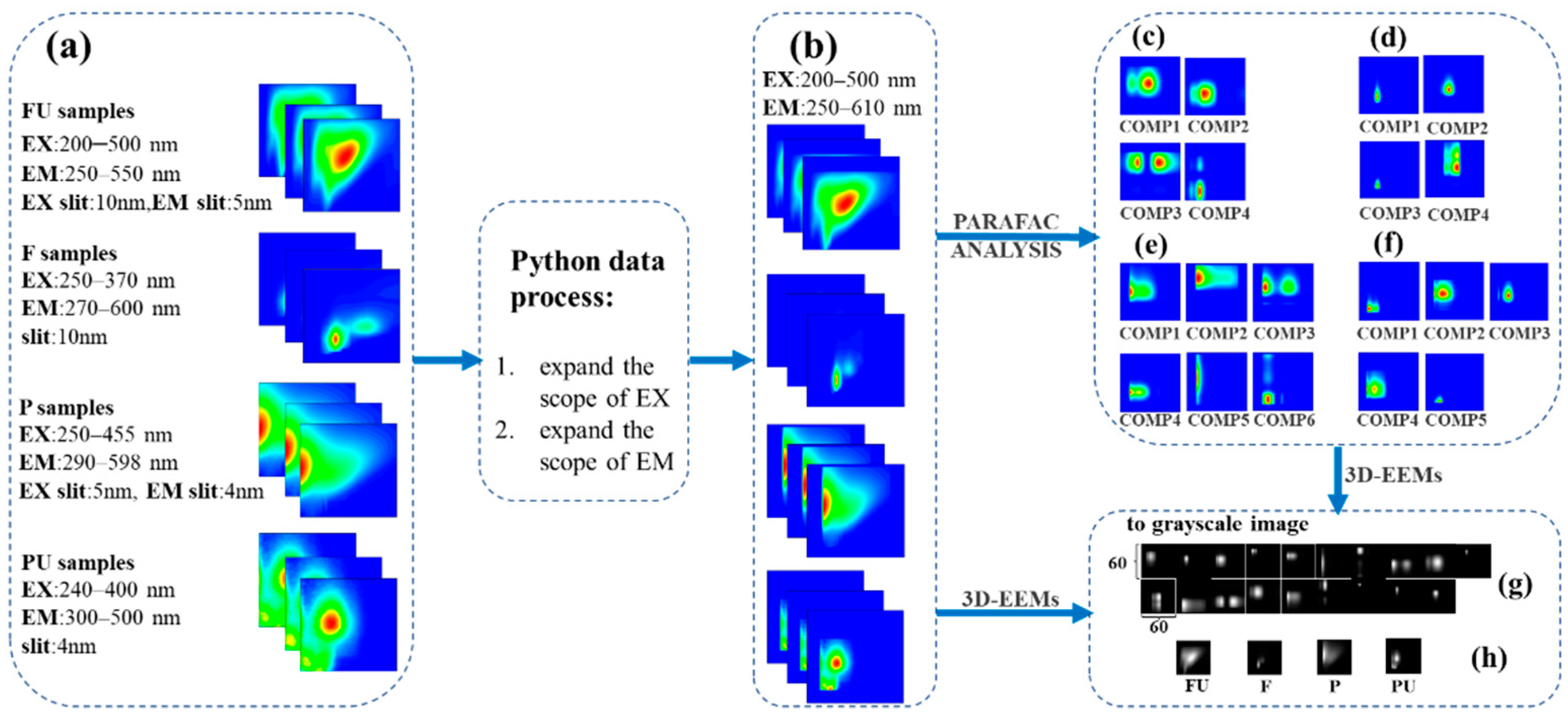
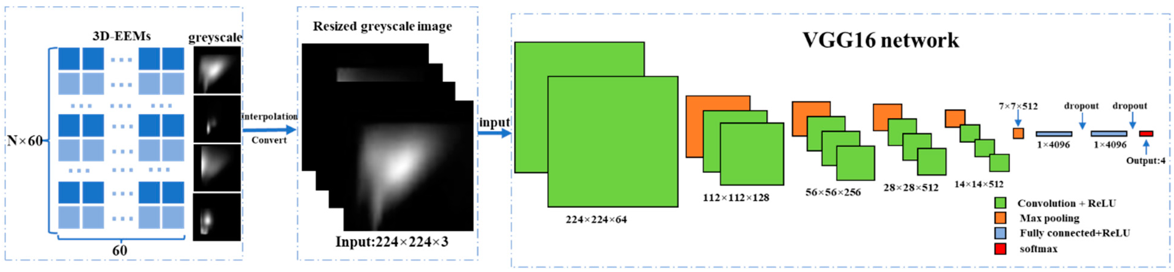
2.3. Data Preprocessing for PARAFAC and CNN
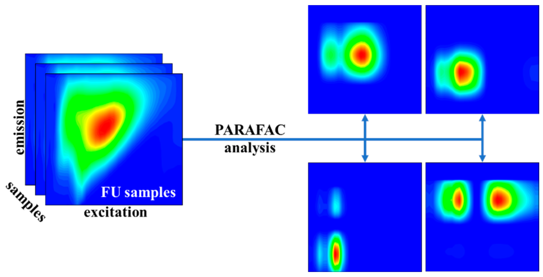
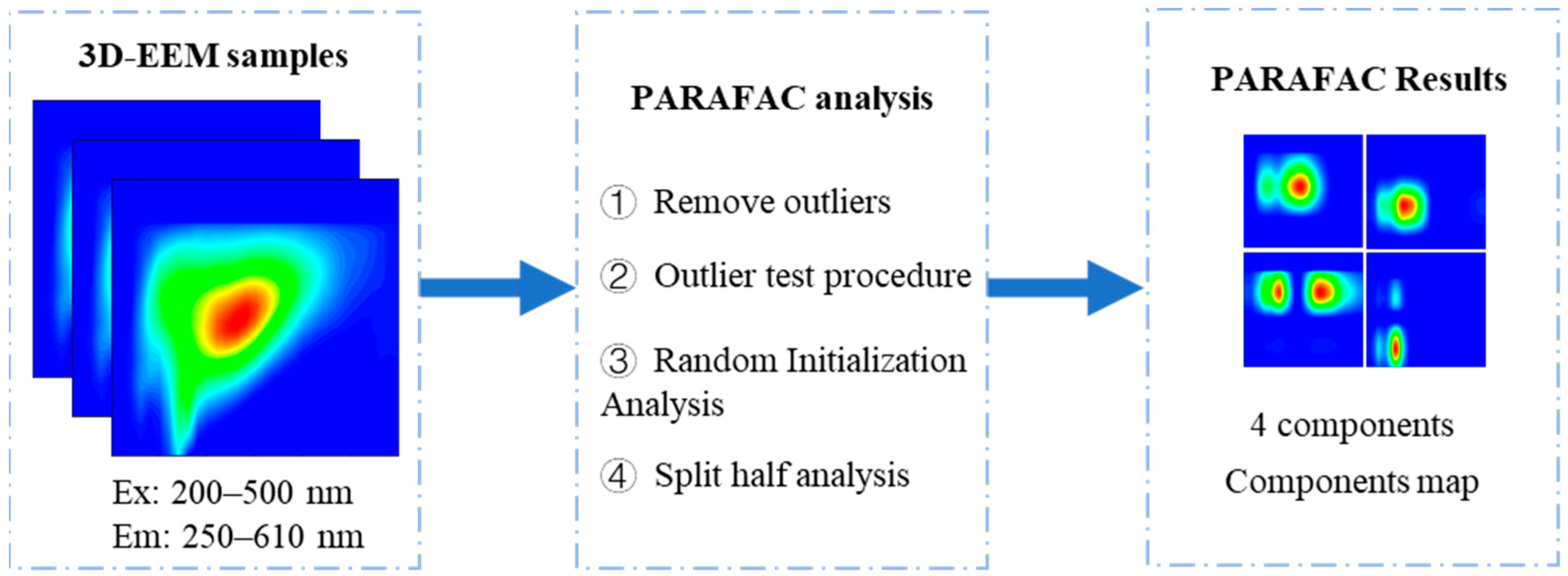
The pre-processing of 3D-EEMs data includes two parts. The first part is to process the original 3D-EEMs data to be suitable for the PARAFAC analysis model’s construction, and the second part is to convert 3D-EEMs data into grayscale images for training and testing of the convolution neural network (CNN) model.
Since these four kinds of data are obtained from different regions and measured with different instruments under different conditions and parameters, they have different excitation and emission wavelength ranges, as well as different excitation and emission intervals. Therefore, it is necessary to adjust the excitation wavelength range and emission wavelength range of the data and normalize the data by using the Raman normalization method [27]. The Pandas and Numpy tools in the Python toolkits were used in this study to unify the excitation spectra interval to 200–500 nm and the emission spectra interval to 250–610 nm (The reason is that this interval contains the common interval of all different datasets to ensure that the fluorescence characteristics of all samples are not lost). In addition, Raman normalization of the data after the interval unification is required. The reference formula for Raman normalization information is as follows:
A r p λ e x = λ e m 1 λ e m 2 I λ e m d λ e m  
F λ e x , λ e m ( R . U . ) = I λ e x , λ e m ( A . U . ) A r p  
In the formula,   I λ   is the spectral correction intensity of the Raman peak at the emission wavelength λ. In this paper,   A r p   is the integral value of the fluorescence intensity of emission ranges from 365–430 nm (excitation = 350 nm).   F is the fluorescence intensity after Raman normalization. A . U .   stands for the arbitrary unit, R . U .   stands for Raman unit.
The pre-processed 3D fluorescence data can be used for PARAFAC analysis, while the processed data and the results of the PARAFAC analysis are normalized and converted into grayscale images, as is shown in the following Figure 2.

2.4. PARAFAC Method

We performed a PARAFAC analysis of the 3D fluorescence data using the drEEM toolbox v0.6. The principle of the PARAFAC analysis method is to decompose the 3D fluorescence data into a set of trilinear terms and a residual array structure [28] (as is shown in the following Figure 3), which is modeled by the process of minimizing the sum of squares of the residuals. Its mathematical expression is as follows:
x i j k = f = 1 F a i f b i f c k f + ε i j k  
i = 1 ,   , I ; j = 1 , , J ; k = 1 , , K  
where, x i j k   is the fluorescence intensity of sample i at emission wavelength j and excitation wavelength k . a i f is directly proportional to the concentration of the f —the analyte in sample i . b i f is linearly related to the fluorescence quantum efficiency of the f —the analyte in sample i . c k f is linearly proportional to the specific absorption coefficient at the excitation wavelength k . F is defined as the number of components of the model and the residual matrix ε i j k represents the variability not considered in the model.

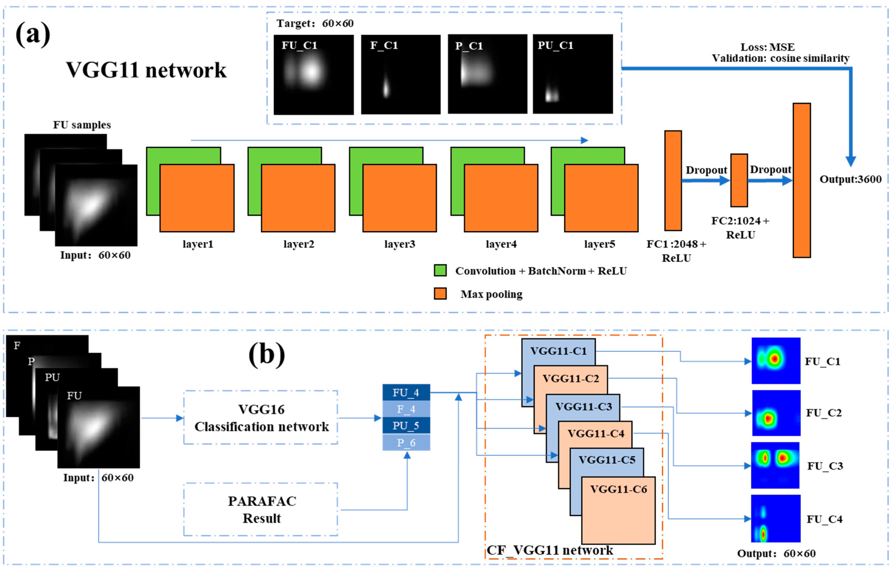
2.5. VGG16 Classification Network

In this study, VGG16 was chosen as the backbone of the 3D fluorescence samples classification network model, and the model diagram is shown below in Figure 4.
The VGG16 network consists of 13 convolution layers and 3 fully connected layers. In this paper, the VGG16 model’s input size is 1 × 224 × 224 pixels (grayscale image), and the cross-entropy function is used as the loss function for model training, and the model training is optimized by Adam optimizer. The cross-entropy loss function is formulated as follows:
L = 1 N i L i = 1 N i c = 1 M y i c log ( p i c )
where M represents the number of categories. y i c   represents the symbolic function (0 or 1). If the real category of sample i is equal to c , take 1, otherwise, take 0.   p i c represents the prediction probability that the observation sample i belongs to category c .
Before training the VGG16 network using 3D-EEMs data, we need to preprocess the 3D-EEMs data to conform to the input and output requirements of the VGG16 network. Through the previous data preprocessing section, the four types of 3D fluorescence datasets have been adjusted to a unified excitation–emission interval, and the Raman normalization operation has been performed on samples. Although this operation was completed, since the excitation interval and emission interval of fluorescence measurement equipment were different during the measurement process of 3D-EEMs, we need to adjust the interval of four types of 3D-EEMs data to be consistent by using interpolation. After interpolation, the size of 3D-EEMs is uniformly transformed to 60 × 60. Figure 5 shows the changes in 3D-EEMs data before and after interpolation. The interpolation method uses bilinear interpolation and the mathematical expression is as follows:
f ( R 1 ) = x 2 x x 2 x 1 f ( Q 11 ) + x x 1 x 2 x 1 f ( Q 21 )
f ( R 2 ) = x 2 x x 2 x 1 f ( Q 12 ) + x x 1 x 2 x 1 f ( Q 22 )
where f ( Q 11 ) ,  f ( Q 21 ) , f ( Q 12 ) and f ( Q 22 ) represent the values of function f at 4 points:   Q 11 = ( x 1 , y 1 ), Q 12 = ( x 1 , y 2 ), Q 21 = ( x 2 , y 1 ), and Q 22 = ( x 2 , y 2 ). In our experiment, x   represents the position of emission–excitation wavelength, and   f   represents the fluorescence intensity at a certain position.
After data normalization, use Python code to convert 3D-EEMs into grayscale images (1 × 60 × 60). The emission interval is the length of the grayscale image, and the excitation interval is the width of the grayscale image, and the fluorescence intensity is the grayscale value. The transformation relationship is as follows:
y = x x m i n x m a x x m i n 255  
where x represents the intensity value of fluorescence in 3D-EEMs, and y represents the grayscale value after conversion to a grayscale image. The data are linearly mapped to the [0, 1] interval using dispersion standardization. x m i n is the minimum fluorescence intensity, x m a x is the maximum fluorescence intensity.

2.6. CF-VGG11 Network

After using the VGG16 network to classify the 3D fluorescence, we can know the type and number of components of 3D-EEMs. Then we used the improved components fitting network CF-VGG11 (Components Fitting VGG11 network) as a model for 3D fluorescence components mapping analysis, which is used to fit the component maps of 3D fluorescence samples. The single model structure of the CF-VGG11 network used in this study is shown below in Figure 6a,b, which shows the structure of the entire network model in this paper. CF-VGG11 network contains six improved sub-VGG11 network structures (determined by the largest components of each type of 3D-EEMs), in which each sub-model is responsible for fitting one component of various 3D fluorescence data. Compared with the original VGG11 network structure, the CF-VGG11 network structure is optimized and adjusted in this paper by adding a dropout layer after the first fully connected layer and the second fully connected layer to enhance the stability of the model and prevent overfitting.
The same as the VGG16 used in this study, CF-VGG11 receives the input as a 1 × 60 × 60 grayscale image and outputs a vector of size 3600 (it can be understood that the channel × length × width: 1 × 60 × 60), and the vector represents the fluorescence intensity value of the component map. In this study, the four datasets used for CF-VGG11 are analyzed by PARAFAC analysis. FU, F, PU, and P have 4 components, 4 components, 5 components, and 6 components, respectively, then the components of each type of 3D-EEMs are numbered, respectively, from C1–C6, using components maps (C1–C6) as the target (label) values for CF-VGG11 training. In the CF-VGG11 model, the mean square error MSE was used as the loss function, the cosine similarity was used as the judgment standard of the model fitting results, and the Adam optimizer was used to optimize the model training [30].
In summary, the network model, and (3) training CF-VGG11 component fitting network model. A 3D-EEM, after removing Raman scattering, removing Rayleigh scattering, and using Raman normalization corrected, as a grayscale image inputting into the VGG16 classification experiment of using a convolutional neural network to analyze 3D fluorescence in this study includes three parts: (1) data preprocessing (PARAFAC analysis and preparation of input data for the CNN model), (2) training VGG16 classification network, combining with the PARAFAC analysis results, so the classification network can derive the category and the number of components. Based on the number of components obtained from the classification, the 3D-EEM, which is previously transmitted to the VGG16 network, is now transmitted to each sub-network of the CF-VGG11 network again, so that the component maps of the 3D-EEM can be obtained.

3. Results and Discussion

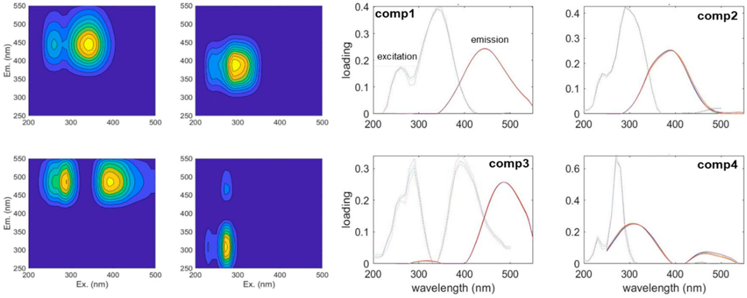
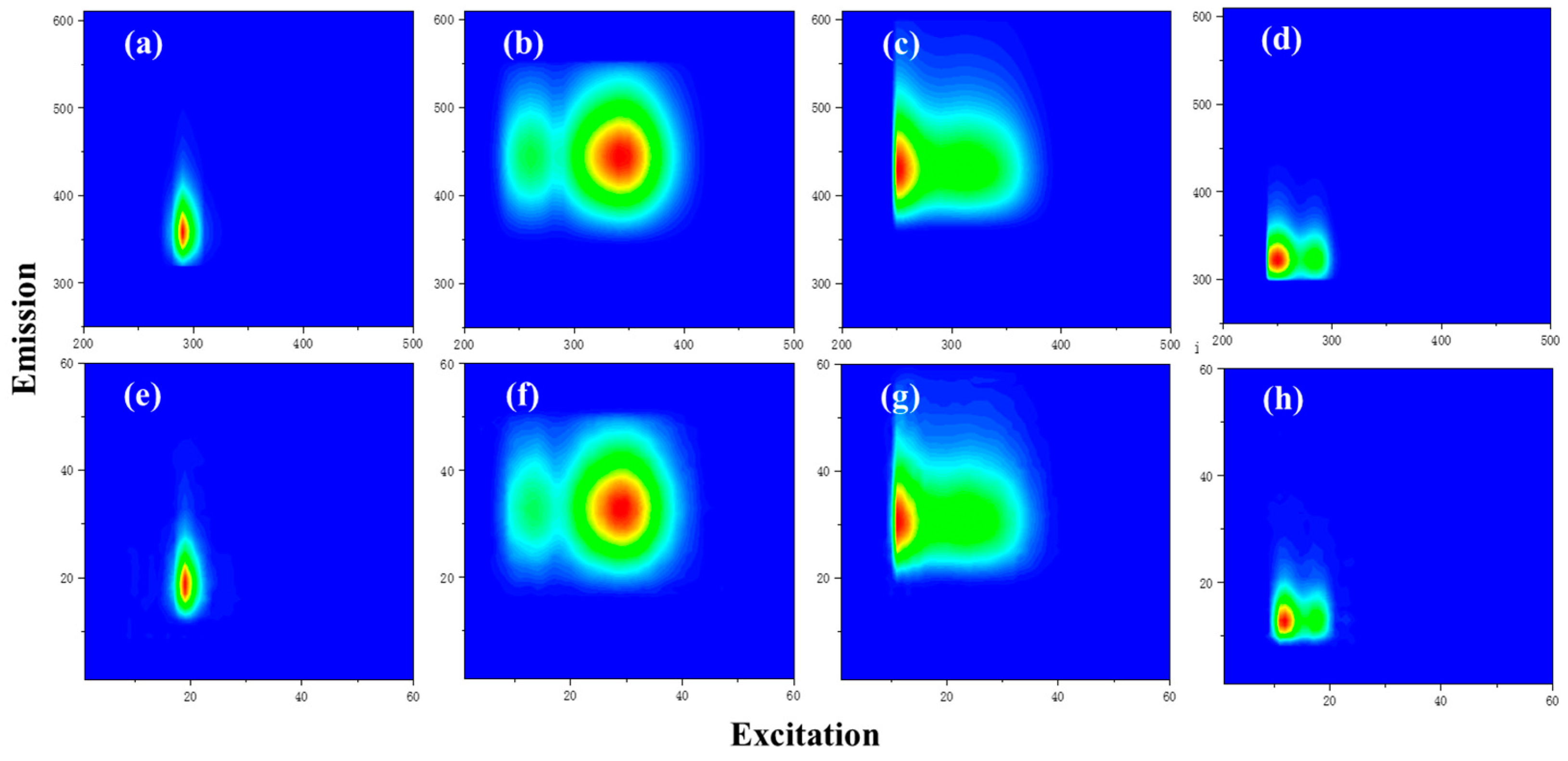
3.1. The Results of the PARAFAC Analysis

In this study, 3D-EEMs were analyzed by the PARAFAC method, which will obtain the correct component number and component maps of 3D fluorescence data [31]. We collected a total of four types of 3D fluorescence data online as well as through field sampling, including a total of 416 samples, with the least amount of FU datasets containing 45 samples. PARAFAC analysis requires a split-half test analysis, so a data volume greater than 21 is more appropriate [32].
After the analysis of these four types of datasets by PARAFAC analysis, four components (FU), four components (F), five components (PU), and six components (P) were obtained, respectively. PARAFAC analysis is conducted separately for each type of dataset. The process of analysis and component maps are shown in Figure 7.
In the experiment we performed PARAFAC analysis on all datasets (Figure 8 and Table 2 show the results of the PARAFAC analysis on FU dataset). Then, we uploaded the PARAFAC results to the OpenFluor database [33] for comparison and obtained the possible matter of these four 3D fluorescence components. Among them, the comparison results show that the similarity scores of components exceed 95% except component-three (94%).
The characteristics of C1 were characterized by a peak at 350 nm excitation with 440 nm emission wavelengths and associated with a group of high molecular weight and aromatic molecules of terrestrial origin [34]. The characteristics of C2 were characterized by a peak at 300 nm excitation with 400 nm emission wavelengths, which is sensitive to the UV-A humic-like and low molecular weight [35]. The characteristics of C3 were characterized by a peak at 290 nm and 400 nm excitations with 480 nm emission wavelengths, which is similar to the humic-like [35]. The characteristics of C4 were characterized by a peak at 280 nm excitation with 320 nm emission wavelengths, which is similar to autochthonous protein-like, and sensitive to microbial degradation [36,37].

3.2. Training and Validation of the VGG16 Network and the CF-VGG11 Network

The training set and validation set used for VGG16 contains 333 samples and the test set contains 83 samples, at a ratio of 6:2:2 (Table 3). In the actual training process, we expanded the images by gamut distortion and mirror flipping. Although the transformed images can not represent the 3D fluorescence characteristics, it can improve the training efficiency of the model and prevent the poor training effect due to the lack of data. The VGG16 classification network was evaluated by using the cross-entropy loss function and training accuracy. We trained the network with 100 epochs and set the initial learning rate of the first 50 epochs to 1.0 × 10⁻³ and the last 50 epochs to 1.0 × 10⁻⁴. We use the stepLR method to automatically update the learning rate. The optimizer adopts the Adam optimizer, with the step parameter set to one and the gamma parameter set to 0.94. In addition, the input size of the network is 224 × 224, the output is 4 classes, the batch_size of the first 50 epochs is set to 8, and the batch_size of the last 50 epochs is set to 16. During the training process, the training loss and validation loss decrease gradually, and the training loss value tends to be stable after 80 epochs. The training loss and validation loss curve is shown in Figure 9. After 5 repeat experiments, as the training logs, we take the best epoch of all as the training result. The loss value is: 2.39 × 10⁻² (training loss) and 1.03 × 10⁻³ (validation loss). Then, we tested the accuracy of the model using the test set samples and the top-5 accuracy is 100%. In the dataset, the test set has a small amount and few types, so the appearance of the test accuracy is good. This is a normal training result since the network can always distinguish the 3D-EEM types well. At the same time, we used the PCA + SVM method (Figure 10) to reduce the dimension and classify 3D-EEMs with an accuracy of 99.69%. However, the PCA + SVM approach has the same requirements as the PARAFAC analysis method, which requires a large amount of data as inputs, so the convolutional neural network has greater advantages (Table 4). The training results show that there are significant differences between different classes of 3D-EEMs and using the convolutional neural network can easily identify the type of 3D-EEMs and the number of their components.
The CF-VGG11 network structure contains six VGG11 network model structures (Figure 5), where each submodel gets a corresponding one component map of each of four datasets based on 3D-EEMs. We used the VGG11 model to fit a component map, which is a vector of size 60 × 60 (it is not an output class), we could not judge the results by the method of traditional target detection and object recognition algorithms, so we used cosine similarity [38] to replace the accuracy of the model fitting results. We divided the data in a ratio of 3:1:1 (250 samples for training and 83 samples for validation and 83 samples for test) and input each 3D-EEM datum into each sub-model while the fitting component map of each model is given by the PARAFAC analysis results. The results of model training are shown in Figure 11.

3.3. Model Performance

To show that the trained VGG16 and CF-VGG11 models have a good fitting performance, we selected some 3D fluorescence data for testing, and the components fitted by the CF-VGG11 model were compared with those analyzed by PARAFAC (Figure 12). It can be seen from the figure that the results fitted by the model are very similar to those obtained by the PARAFAC analysis method, with the difference that there are a few noise points in the results fitted by the model, and these noise points do not have much effect on the components of 3D-EEMs. Therefore, we can conclude that VGG16 and CF-VGG11 can be well classified and fitted according to 3D-EEMs.

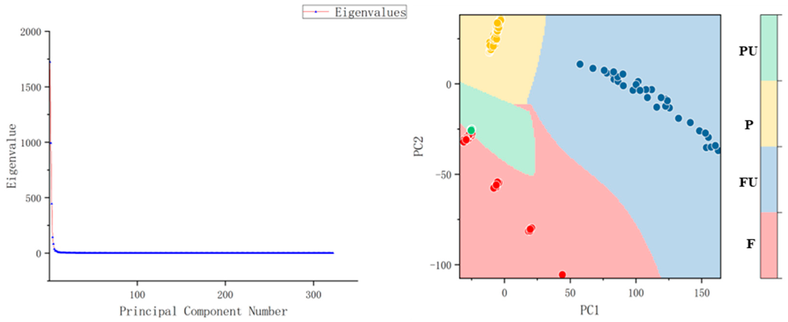
3.4. Comparison between the VGG Network and the PARAFAC Analysis Method

Our convolutional neural networks are based on the PARAFAC analysis method. We need the PARAFAC analysis method to provide the correct number of components and component maps, and the network is trained on these correct data for the final purpose of 3D-EEMs classification and component map fitting.
In addition, our models of VGG16 and CF-VGG11 have some advantages over the PARAFAC analysis in that the models require only one 3D-EEM input to obtain the correct sample category and its component maps. This is of great application value in scenarios where rapid 3D-EEMs analysis needs to be established. The specific comparison between PARAFAC and our model is shown in Table 5.
In recent years, many people have tried to use 3D fluorescence data for the rapid analysis of river water [39,40] to characterize the DOM pollution of river water. The model based on this study can achieve the purpose of rapid analysis of river water.

4. Conclusions

In conclusion, we use VGG16 to accurately classify 3D-EEMs and use the CF-VGG11 model to realize the component maps fitting different kinds of 3D-EEMs. The model relies on PARAFAC analysis for preliminary data preparation, but it can overcome the problem of strict data requirements of PARAFAC in the process of use and provides a new analytical tool for the real-time 3D fluorescence analysis of small samples.

Author Contributions

Methodology, S.Z. and X.J.; Project administration, K.R.; Resources, Y.L. and T.L.; Supervision, J.F., D.O., Q.T. and J.X.; Writing—original draft, K.R.; Writing—review & editing, K.R., X.J. and Z.L. All authors have read and agreed to the published version of the manuscript.

Funding

This research was funded by Key R & D projects of Fund of Technical Office in Sichuan Province, grant number 2021YFS0279.

Data Availability Statement

The datasets, PARAFAC analysis results, CNN model can be found here: https://github.com/qkmc-rk/VGG16-CF-VGG11.git, accessed on 5 April 2022.

Conflicts of Interest

The authors declare no conflict of interest.

References

  1. Hu, B.; Ma, Y.; Wang, N. A novel water pollution monitoring and treatment agent: Ag doped carbon nanoparticles for sensing dichromate, morphological analysis of Cr and sterilization. Microchem. J. 2020, 157, 104855. [Google Scholar] [CrossRef]
  2. Zhong, R.S.; Zhang, X.H.; Guan, Y.T.; Mao, X.Z. Three-Dimensional Fluorescence Fingerprint for Source Determination of Dissolved Organic Matters in Polluted River. Spectrosc. Spectr. Anal. 2008, 28, 347–351. [Google Scholar]
  3. Duan, P.; Wei, M.; Yao, L.; Li, M. Relationship between non-point source pollution and fluorescence fingerprint of riverine dissolved organic matter is season dependent. Sci. Total Environ. 2022, 823, 153617. [Google Scholar] [CrossRef] [PubMed]
  4. Gunnarsdottir, M.J.; Gardarsson, S.M.; Figueras, M.J.; Puigdomènech, C.; Juárez, R.; Saucedo, G. Water safety plan enhancements with improved drinking water quality detection techniques. Sci. Total Environ. 2020, 698, 134185. [Google Scholar] [CrossRef] [PubMed]
  5. Rizk, R.; Alameraw, M.; Rawash, M.A.; Juzsakova, T.; Domokos, E.; Hedfi, A.; Almalki, M.; Boufahj, F.; Gabriel, P.; Shafik, H.M.; et al. Does the Balaton Lake affected by pollution? Assessment through Surface Water Quality Monitoring by using different assessment methods. Saudi J. Biol. Sci. 2021, 28, 5250–5260. [Google Scholar] [CrossRef]
  6. Baghoth, S.A.; Sharma, S.K.; Amy, G.L. Tracking natural organic matter (NOM) in a drinking water treatment plant using fluorescence excitation–emission matrices and PARAFAC. Water Res. 2011, 45, 797–809. [Google Scholar] [CrossRef]
  7. Shi, F. Research on Open-Set Recognition of Organic Pollutants in Water Based on 3D Fluorescence Spectroscopy; Zhejiang University: Zhejiang, China, 2021. [Google Scholar]
  8. Xu, R.Z.; Cao, J.S.; Feng, G.; Luo, J.Y.; Feng, Q.; Ni, B.J.; Fang, F. Fast identification of fluorescent components in three-dimensional excitation-emission matrix fluorescence spectra via deep learning. Chem. Eng. J. 2022, 430, 132893. [Google Scholar] [CrossRef]
  9. Xu, R.Y.; Zhu, Z.W.; Hu, Y.J.; Zhang, Y.; Chen, G.Q. The Discrimination of Chinese Strong Aroma Type Liquors with Three-Dimensional Fluorescence Spectroscopy Combined with Principal Component Analysis and Support Vector Matchine. Spectrosc. Spectr. Anal. 2016, 36, 1021–1026. [Google Scholar]
  10. Zhang, H.; Li, H.; Gao, D.; Yu, H. Source identification of surface water pollution using multivariate statistics combined with physicochemical and socioeconomic parameters. Sci. Total Environ. 2022, 806, 151274. [Google Scholar] [CrossRef]
  11. Andersen, C.M.; Bro, R. Practical aspects of PARAFAC modeling of fluorescence excitation-emission data. J. Chemom. 2003, 17, 200–215. [Google Scholar] [CrossRef]
  12. ECarstea, M.; Bridgeman, J.; Baker, A.; Reynolds, D.M. Fluorescence spectroscopy for wastewater monitoring: A review. Water Res. 2016, 95, 205–219. [Google Scholar] [CrossRef] [PubMed]
  13. Yang, C.; Liu, Y.; Sun, X.; Miao, S.; Guo, Y.; Li, T. Characterization of fluorescent dissolved organic matter from green macroalgae (Ulva prolifera)-derived biochar by excitation-emission matrix combined with parallel factor and self-organizing maps analyses. Bioresour. Technol. 2019, 287, 121471. [Google Scholar] [CrossRef] [PubMed]
  14. Gu, W.; Huang, S.; Lei, S.; Yue, J.; Su, Z.; Si, F. Quantity and quality variations of dissolved organic matter (DOM) in column leaching process from agricultural soil: Hydrochemical effects and DOM fractionation. Sci. Total Environ. 2019, 691, 407–416. [Google Scholar] [CrossRef] [PubMed]
  15. Lee, B.M.; Seo, Y.S.; Hur, J. Investigation of adsorptive fractionation of humic acid on graphene oxide using fluorescence EEM-PARAFAC. Water Res. 2015, 73, 242–251. [Google Scholar] [CrossRef] [PubMed]
  16. Li, L.; Wang, Y.; Zhang, W.; Yu, S.; Wang, X.; Gao, N. New advances in fluorescence excitation-emission matrix spectroscopy for the characterization of dissolved organic matter in drinking water treatment: A review. Chem. Eng. J. 2020, 381, 122676. [Google Scholar] [CrossRef]
  17. Chen, W.; Westerhoff, P.; Leenheer, J.A.; Booksh, K. Fluorescence excitation—Emission matrix regional integration to quantify spectra for dissolved organic matter. Environ. Sci. Technol. 2003, 37, 5701–5710. [Google Scholar] [CrossRef] [PubMed]
  18. Yamashita, Y.; Jaffé, R. Characterizing the interactions between trace metals and dissolved organic matter using excitation—Emission matrix and parallel factor analysis. Environ. Sci. Technol. 2008, 42, 7374–7379. [Google Scholar] [CrossRef]
  19. Guimet, F.; Ferré, J.; Boqué, R.; Rius, F.X. Application of unfold principal component analysis and parallel factor analysis to the exploratory analysis of olive oils by means of excitation–emission matrix fluorescence spectroscopy. Anal. Chim. Acta 2004, 515, 75–85. [Google Scholar] [CrossRef]
  20. Peiris, R.H.; Hallé, C.; Budman, H.; Moresoli, C.; Peldszus, S.; Huck, P.M.; Legge, R.L. Identifying fouling events in a membrane-based drinking water treatment process using principal component analysis of fluorescence excitation-emission matrices. Water Res. 2010, 44, 185–194. [Google Scholar] [CrossRef]
  21. Cuss, C.W.; McConnell, S.M.; Guéguen, C. Combining parallel factor analysis and machine learning for the classification of dissolved organic matter according to source using fluorescence signatures. Chemosphere 2016, 155, 283–291. [Google Scholar] [CrossRef]
  22. Wu, X.; Zhao, Z.; Tian, R.; Shang, Z.; Liu, H. Identification and quantification of counterfeit sesame oil by 3D fluorescence spectroscopy and convolutional neural network. Food Chem. 2020, 311, 125882. [Google Scholar] [CrossRef] [PubMed]
  23. Lu, Z.; Li, J.; Ruan, K.; Sun, M.; Zhang, S.; Liu, T.; Yin, J.; Wang, X.; Chen, H.; Wang, Y.; et al. Deep learning-assisted smartphone-based ratio fluorescence for “on–off-on” sensing of Hg2+ and thiram. Chem. Eng. J. 2022, 435, 134979. [Google Scholar] [CrossRef]
  24. Liu, T.; Chen, S.; Ruan, K.; Zhang, S.; He, K.; Li, J.; Chen, M.; Yin, J.; Sun, M.; Wang, X.; et al. A handheld multifunctional smartphone platform integrated with 3D printing portable device: On-site evaluation for glutathione and azodicarbonamide with machine learning. J. Hazard. Mater. 2022, 426, 128091. [Google Scholar] [CrossRef] [PubMed]
  25. Murphy, K.R.; Stedmon, C.A.; Graeber, D.; Bro, R. Fluorescence spectroscopy and multi-way techniques. PARAFAC. Anal. Methods 2013, 5, 6557–6566. [Google Scholar] [CrossRef] [Green Version]
  26. Yang, Y.Z.; Peleato, N.M.; Legge, R.L.; Andrews, R.C. Fluorescence excitation emission matrices for rapid detection of polycyclic aromatic hydrocarbons and pesticides in surface waters. Environ. Sci. Water Res. Technol. 2019, 5, 315–324. [Google Scholar] [CrossRef]
  27. Lawaetz, A.J.; Stedmon, C.A. Fluorescence intensity calibration using the Raman scatter peak of water. Appl. Spectrosc. 2009, 63, 936–940. [Google Scholar] [CrossRef]
  28. Stedmon, C.A.; Markager, S.; Bro, R. Tracing dissolved organic matter in aquatic environments using a new approach to fluorescence spectroscopy. Mar. Chem. 2003, 82, 239–254. [Google Scholar] [CrossRef]
  29. Dagar, A.; Nandal, D. High performance Computing Algorithm Applied in Floyd Steinberg Dithering. Int. J. Comput. Appl. 2012, 43, 0975–8887. [Google Scholar]
  30. Niu, C.; Tan, K.; Jia, X.; Wang, X. Deep learning based regression for optically inactive inland water quality parameter estimation using airborne hyperspectral imagery. Environ. Pollut. 2021, 286, 117534. [Google Scholar] [CrossRef]
  31. Bro, R. PARAFAC. Tutorial and applications. Chemom. Intell. Lab. Syst. 1997, 38, 149–171. [Google Scholar] [CrossRef]
  32. Murphy, K.R.; Hambly, A.; Singh, S.; Henderson, R.K.; Baker, A.; Stuetz, R.; Khan, S.J. Organic Matter Fluorescence in Municipal Water Recycling Schemes: Toward a Unified PARAFAC Model. Environ. Sci. Technol. 2011, 45, 2909–2916. [Google Scholar] [CrossRef] [PubMed]
  33. Murphy, K.R.; Stedmon, C.A.; Wenig, P.; Bro, R. Openfluor- an online spectral library of auto-fluorescence by organic compounds in the environment. Anal. Methods 2014, 6, 658–661. [Google Scholar] [CrossRef] [Green Version]
  34. Chen, B.; Huang, W.; Ma, S.; Feng, M.; Liu, C.; Gu, X.; Chen, K. Characterization of Chromophoric Dissolved Organic Matter in the Littoral Zones of Eutrophic Lakes Taihu and Hongze during the Algal Bloom Season. Water 2018, 10, 861. [Google Scholar] [CrossRef] [Green Version]
  35. Kothawala, D.; von Wachenfeldt, E.; Koehler, B.; Tranvik, L. Selective loss and preservation of lake water dissolved organic matter fluorescence during long-term dark incubations. Sci. Total Environ. 2012, 433, 238–246. [Google Scholar] [CrossRef] [PubMed]
  36. Osburn, C.L.; Wigdahl, C.R.; Fritz, S.C.; Saros, J.E. Dissolved organic matter composition and photoreactivity in prairie lakes of the U.S. Great plains. Limnol. Oceanogr. 2011, 56, 2371–2390. [Google Scholar] [CrossRef] [Green Version]
  37. Li, P.; Chen, L.; Zhang, W.; Huang, Q. Spatiotemporal distribution, sources, and photobleaching imprint of dissolved organic matter in the Yangtze estuary and its adjacent sea using fluorescence and parallel factor analysis. PLoS ONE 2015, 10, e0130852. [Google Scholar] [CrossRef]
  38. Tang, J.; Wu, J.; Li, Z.; Cheng, C.; Liu, B.; Chai, Y.; Wang, Y. Novel insights into variation of fluorescent dissolved organic matters during antibiotic wastewater treatment by excitation emission matrix coupled with parallel factor analysis and cosine similarity assessment. Chemosphere 2018, 210, 843–848. [Google Scholar] [CrossRef]
  39. Zhang, F.; Wang, X.; Chen, Y.; Airiken, M. Estimation of surface water quality parameters based on hyper-spectral and 3D-EEM fluorescence technologies in the Ebinur Lake Watershed, China. Phys. Chem. Earth Parts A/B/C 2020, 118, 118–119. [Google Scholar] [CrossRef]
  40. Zeng, W.; Qiu, J.; Wang, D.; Wu, Z.; He, L. Ultrafiltration concentrated biogas slurry can reduce the organic pollution of groundwater in fertigation. Sci. Total Environ. 2022, 810, 151294. [Google Scholar] [CrossRef]
Figure 1. FU dataset sampling sites. The sequence of sampling sites shall be sorted according to the sampling time. The number of samples collected from each site are: Site 1 collected 10 samples, Site 2 collected 5 samples, Site 3 collected 3 samples, Site 4 collected 3 samples, Site 5 collected 3 samples, Site 6 collected 3 samples, Site 7 collected 8 samples, Site 8 collected 2 samples, Site 9 collected 2 samples, and Site 10 collected 10 samples. The number of samples shall be determined according to the actual situation of the sampling sites.
Applsci 12 04886 g001
Figure 2. (a) Corrected data by Raman normalization; (b) Adjust the excitation ranges to: 200–550 nm, emission: 250–610 nm; (c) FU components (PARAFAC results); (d) F components; (e) P component; (f) PU components; (g) Grayscale image of 3D-EEMs components; and (h) Original 3D-EEMs grayscale image. This figure shows the data processing method in this paper, in which the grayscale images are generated by the samples EEMs and components EEMs, rather than the contour image, and pixels represent fluorescence intensity. In (b), the reason why the range is set as this range is to preserve the characteristic information of all 3D-EEMs. By using the bilinear interpolation method to interpolate 3D-EEMs, the size of the gray image is 60 × 60.
Applsci 12 04886 g002
Figure 3. 3D-EEMs are decomposed into PARAFAC components.
Applsci 12 04886 g003
Figure 4. 3D-EEMs classification network based on VGG16. The size of the image is interpolated from size (60 × 60) to size (224 × 224) using the bilinear interpolation method. Grayscale images are converted into 3-channel RGB images using the Python Pillow function: Image.convert (“RGB”), which uses the Floyd–Steinberg dither method [29].
Applsci 12 04886 g004
Figure 5. Comparison before and after 3D-EEMs interpolation. (a) Before interpolation; and (b) After interpolation. In (b), emission and excitation from 1 to 60 represent the number of wavelengths and excitation wavelengths, and the range of wavelengths is still consistent with that in (a).
Applsci 12 04886 g005
Figure 6. (a) is the single-layer network structure of VGG11; (b) is the structure of the whole fitting network. In (a), the input is a grayscale image of size 60 × 60 and the output is a vector of size 3600. The output vector can be reshaped as a matrix of size 60 × 60. VGG11 network contains 5 convolution-batch norm-pooling layers and 3 fully connected layers. The first and second fully connected layers are followed by a dropout layer, which can prevent the network from overfitting. VGG11 network is trained by the MSE loss function, and the training effect is verified by the cosine similarity. FU_C1 in this figure represents 1st component map of FU, as the other 3 component maps. Each layer represents a group of “convolution-batch norm-relu-Max pooling”. Input is the grayscale image of the network (taking the FU sample as an example), and the target is the label fitted by the convolution network. In (b), four types of 3D-EEMs samples are first classified by the VGG16 classification network. After obtaining the classification results, combined with the component map number from PARAFAC analysis, the classification results and original 3D-EEMs are input into the CF-VGG11 network, and the component maps of 3D-EEMs can be obtained through CF-VGG11 network fitting. Among them, FU_4 indicates that the FU samples contain 4 component maps. VGG11-C1 represents the convolution network used to fit the first component. By inputting each type of 3D-EEMs to VGG11-C1, the first component map of each type of data can be obtained, which is similar to the other 5 subnetworks of CF-VGG11.
Applsci 12 04886 g006
Figure 7. PARAFAC analysis process and result (taking FU dataset as an example).
Applsci 12 04886 g007
Figure 8. The results of PARAFAC analysis on FU dataset. The loading maps on the right show the result of split-half validation.
Applsci 12 04886 g008
Figure 9. Loss curve and training accuracy curve of VGG16.In (a), when epoch > 80,the training loss and validation loss are both stable. In (b), the training accuracy reaches 99.6% at epoch 97 (the accuracy also reaches 99.6% at epoch 80 and epoch 81).
Applsci 12 04886 g009
Figure 10. In the PCA experiment, the cumulative of the first three PCs is 87.77%, and the cumulative of the first four PCs is 91.73%. The classification accuracy of SVM is 99.69. The reason for the error is that there are some similar characteristics between PC1 and PC2 of F and PU.
Applsci 12 04886 g010
Figure 11. (a,b) show the loss curves, (c,d) show the cosine similarity of model training. In (a,b), the comparison of loss values, the VGG11 model is better than AlexNet model, while the training loss of LeNet is smaller than that of VGG11 model, but the validation loss of VGG11 model is smaller. A smaller loss value means better network performance. Although these 3 models perform well, the VGG11 model has better and more stable performance. (c) shows the change of cosine similarity during model training. VGG11 network shows the best performance of the 3 models. Through the histogram (d) we can see the training change law in the process of 30–40 epochs.
Applsci 12 04886 g011
Figure 12. (ad) are the first component maps of 4 types of 3D-EEMs analyzed by PARAFAC (other component maps are not listed due to limited space), (eh) are the component maps obtained by CF-VGG11 fitting. In (ad), the abscissa is the excitation wavelength, the ordinate is the emission wavelength, and the fluorescence intensity is the fluorescence intensity after Raman normalization. In (eh), the abscissa = (excitation-200)/5 and the ordinate is (emission-250)/6.
Applsci 12 04886 g012
Table 1. Catalogues of collected 3D-EEMs.
CataloguesLabelNumber
Fu riverFU45
Fish muscle (Andersen et al.)F105
PortSurvey (Murphy et al.)P206
Pure (drEEM Tutorial)PU60
Total416 samples
Table 2. Spectral characteristics of EEMs from comparing result of PARAFAC components and OpenFluor database.
ComponentEXmax/EmmaxDescriptionNumber of OpenFluor Matches
C1350 nm/440 nmterrestrial humic-like, high relative aromaticity and molecular weight [34]21
C2300 nm/400 nmUV-A humic-like, low molecular weight [35]14
C3290 nm, 400 nm/480 nmhumic-like [35]4
C4280 nm/320 nmautochthonous protein-like, sensitive to microbial degradation [36,37]11
Table 3. Samples division table.
SamplesNumberTrainValidateTestTotal Samples after Expansion
FU452799135
F105632121315
P2061244141618
PU60361212180
Total41625083831248
Table 4. Comparison results between VGG16 and PCA + SVM.
MethodTraining Accuracy (%)Sample DemandSpeedOperation
VGG1699.60≥1FastEasy
PCA + SVM99.69ManySlowComplex
Table 5. Comparison between PARAFAC and VGG models (performance).
TrainProgressDataSkillsIntegrate to Apps
PARAFACNoComplex≥21YesComplex
VGG16+CF-VGG11YesEasy≥1NoEasy
Publisher’s Note: MDPI stays neutral with regard to jurisdictional claims in published maps and institutional affiliations.

