Abstract
It is critical to use scientific methods to track the performance degradation of in-service buildings over time and avoid accidents. In recent years, both supervised and unsupervised learning methods have yielded positive results in structural health monitoring (SHM). Supervised learning approaches require data from the entire structure and various damage scenarios for training. However, it is impractical to obtain adequate training data from various damage situations in service facilities. In addition, most known unsupervised approaches for training only take response data from the entire structure. In these situations, contaminated data containing both undamaged and damaged samples, typical in real-world applications, prevent the models from fitting undamaged data, resulting in performance loss. This work provides an unsupervised technique for detecting structural damage for the reasons stated above. This approach trains on contaminated data, with the anomaly score of the data serving as the model’s output. First, we devised a score-guided regularization approach for damage detection to expand the score difference between undamaged and damaged data. Then, multi-task learning is incorporated to make parameter adjustment easier. The experimental phase II of the SHM benchmark data and data from the Qatar University grandstand simulator are used to validate this strategy. The suggested algorithm has the most excellent mean AUC of 0.708 and 0.998 on the two datasets compared to the classical algorithm.
1. Introduction
Structural health monitoring (SHM) is a practical and essential process for assessing the structural integrity of structures to prevent damage from ageing, material deterioration, environmental behavior, poor construction, and natural disasters. The essential technique of structural health monitoring is structural damage detection. Many approaches for detecting damage have been proposed and implemented in recent years. Vibration-based damage detection is among the most productive approaches to detect structural deterioration in general [1]. Vibration-based damage detection approaches can be divided into physical model-based and data-based methods [2]. The measurement data obtained by sensors positioned on the monitored structure is the sole data source for data-based approaches. Data-based methods are more commonly used as structural monitoring tools because they account for the impacts of uncertainty on structural damage [3] and are computationally affordable. Recent advances in computation technology facilitate the development of more complex models for data-based methods by means of so-called deep learning [4], which is characterized by artificial neural networks with high numbers of layers. This allows learning complex non-linear mappings between inputs and outputs from data. These data-based methods can be trained through supervised or unsupervised learning.
In recent years, supervised learning has been widely used in SHM. For example, Abdeljaber et al. [5] applied the supervised learning method based on one-dimensional convolutional neural network (1D-CNN) to successfully verify the recognition performance of 1D-CNN under nine damage conditions. Avci et al. [6] used the trained 1D-CNN to diagnose the damage status of structures. Sergio et al. [7] proposed a new analysis method of building a vulnerability framework based on machine learning and tested and verified the reliability of the established module through the rapid visual scanning support model. Although supervised learning has been found to improve damage detection accuracy, it requires a substantial amount of complete and diverse damage case data for training. Furthermore, manually labelling the enormous amount of data obtained is impractical. Certain researchers have employed finite element models to generate sufficient training data from various decision support systems [8]. However, it is difficult to simulate the environment’s uncertainty and boundary conditions and the nonlinear relationship between the damage level and the variation level of the model properties. Therefore, unsupervised learning is the preferred method for damage detection [9].
Unsupervised learning has been popular in recent years for damage detection. Sarmadi et al. [10] suggested an unsupervised damage detection model for detecting damage in scenarios with environmental variables. This model uses Mahalanobis distance to distinguish different damage states, and performance is validated on laboratory-scale bridges exposed to various damage states. Da Silva et al. [11] adopted an unsupervised clustering method based on Fuzzy c-means (FCM) and Gustafson-Kessel (GK) clustering algorithms to build a model using only data obtained from the entire structure. Damage to a three-layer bookshelf structure is detected using these well-trained models. The damage detection results reveal that all intact cases are classified better than damage cases. The GK algorithm’s performance is superior to that of the FCM method in specific damage circumstances. Adeli et al. [12] extracted characteristics from pre-processed signals of whole states and another set of pre-processed signals of unknown states using Restricted Boltzmann Machines. The raw acceleration signal is processed using a simultaneous compressive wavelet transform and a Fast-Fourier transform. The collected features are then performed to analyze data states.
The one-class support vector machine (OC-SVM) has been frequently employed in damage detection as an unsupervised machine learning method. Long and Buyukozturk [13] used an automated OC-SVM to locate damage locations in a three-story, two-bay steel structure in the laboratory. Wang and Cha [14] integrated OC-SVM with an auto-encoder to detect structural damage in laboratory steel bridges. Only the data from the entire structure is used in their research. The auto-encoders loss error is used as a damage sensitivity factor in training. The proposed method can detect slight damage and has a high detection rate. In addition, cluster-based unsupervised algorithms for structural damage detection are commonly used. Diez et al. [15] suggested an unsupervised structural damage assessment technique based on the K-nearest neighbor algorithm to detect bridge damage. We must manually pre-define the number of clusters K for data clustering in the K-nearest neighbor approach. However, when dealing with high-dimensional and massive training data from various unknown conditions, determining an acceptable value for K can be difficult, and the clustering results are prone to local optimality. Cha et al. [16] suggested an unsupervised learning method that uses a fast-clustering strategy based on density peaks for civil infrastructure damage detection to address the issues raised by conventional clustering-based methods.
In structural damage detection, it is crucial to choose appropriate metrics. Throughout the years, researchers have used many different damage parameters as indicators for judging structural damage status, such as natural frequencies, damping, frequency response function, modal strain energy, etc. Different damage parameters have different application scenarios. The success of structural damage detection algorithms largely depends on the selection of damage parameters, because the estimation of the threshold often has a great relationship with the damage indicators. Fan and Qiao [17] reviewed extensive literature and recommended that modal curvature-based algorithms are more reliable in detecting damage than frequency and modal-based algorithms. Cao et al. [18] concluded that damping is a very effective indicator of damage, especially when combined with frequency or mode shape, provided that appropriate damping measurement techniques can be used. Barman et al. [19] used modal strain energy (DIMSE), frequency response function strain energy dissipation ratio (FRFSEDR), flexibility strain energy damage ratio (FSEDR) and residual force-based damage index (RFBDI) as damage indexes; then, they applied Bayesian data fusion approach to these four damage indexes to find out the accurate damage location. In addition to using damage parameters as metrics, other factors are often used as metrics in unsupervised structural damage methods. Pathirage et al. [20] used the learned feature representations in the hidden layers of the deep auto-encoders as damage sensitive features to indicate the presence of damage in the monitored structures. Wang and Cha [14] used three indexes quantifying the reconstruction losses between the original acceleration response inputs and the reconstructed acceleration response outputs as damage-sensitive features.
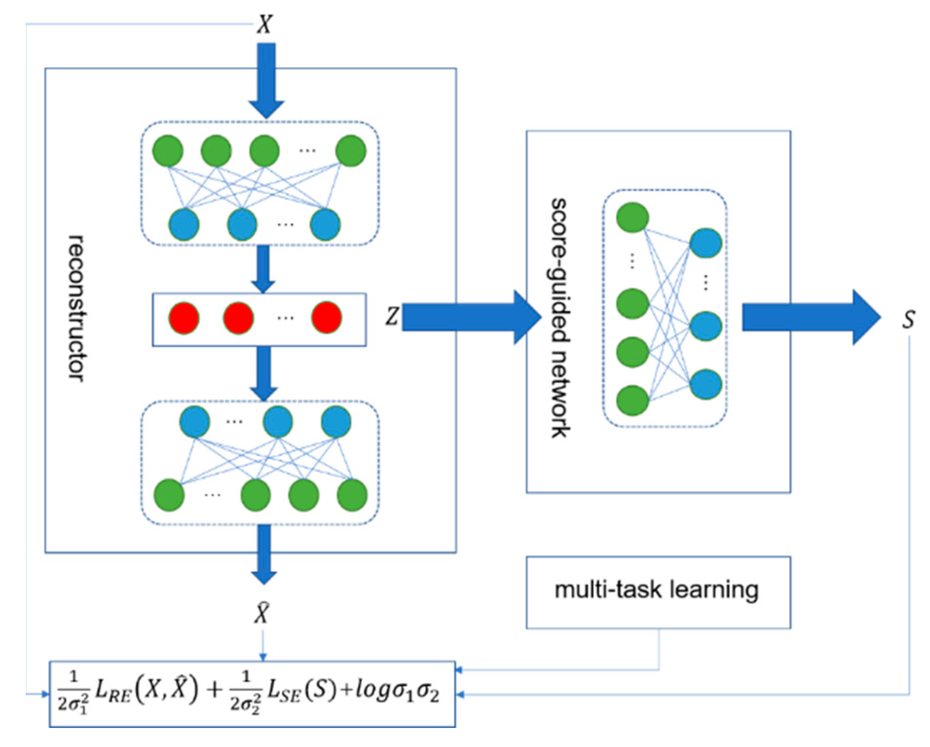
According to our findings, the data employed in many unsupervised structural damage detection algorithms tends to be undamaged. On the other hand, building constructions are frequently exposed to the natural environment, resulting in differing degrees of damage. It is not easy to ensure that the data obtained is entirely undamaged. We also noticed that the selection of suitable damage indicators has the some limitations: (1) When selecting damage parameters as damage indicators, researchers are required to have relevant background knowledge; (2) damage indicators for most unsupervised structural damage detection methods always solely rely on pre-defined distance metrics or reconstruction errors, and thereby cannot be flexibly embedded into other structural damage detection models. As a result, a new unsupervised damage detection method based score-guided regularization strategy is proposed in this study. Figure 1 depicts the basic flow of the score-guided network. The representation learner, which maps the data to the hypothesis space, is connected to the score-guided network, as shown in the diagram. The representation learner is trained to extract more valuable information using the score-guided regularization technique, widening the gap between undamaged and damaged data. This method’s representation learner employs an auto-encoder to extract damage characteristics, while the score-guided network serves as a damaged detector. Finally, multi-task learning is applied to make parameter modification easier. The following are the novelty and significant contributions of our proposed method:
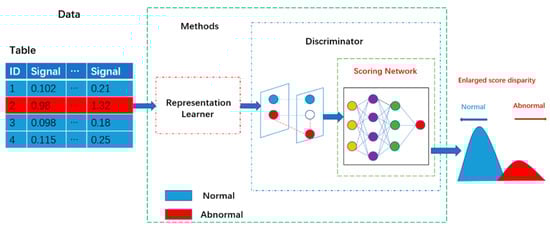
Figure 1.
The basic flow of an unsupervised score-guided network. In this model, the representation learner is simultaneously trained with the scoring network. The scoring network guides the representation learner to learn better discriminative information from the input data.
- (1)
- The proposed method requires contaminated data as training data, which is more realistic than current unsupervised algorithms that solely employ undamaged data.
- (2)
- The model can learn more representative information using a score-guided regularization technique. The difference between undamaged and damaged data is widened by scoring the input data, allowing undamaged and damaged data to be distinguished. The model takes an anomaly score as output. Proposed method selects the anomaly score, that is, the score of the input sample, as the damage indicators, which does not require relevant background knowledge or pre-defined, but is directly output in an end-to-end manner.
- (3)
- Using multi-task learning to simplify the hyperparameter tuning procedure increases the model’s performance and adaptability.
There are four sections in this paper. The “Introduction” section introduces and evaluates existing unsupervised structural damage detection algorithms. Section 2 explains the unique unsupervised structural damage detection algorithm. The suggested algorithm is validated in Section 3 using two benchmark datasets. Section 4 summarizes the entire text and suggests future research areas.
2. Proposed Method
2.1. Model
This section describes the suggested unsupervised structural damage detection method in detail. The method extracts feature with a deep auto-encoder and then employs a score-guided regularization strategy to widen the anomaly score difference between undamaged and damaged data. It also employs multi-task learning to fine-tune the network’s hyperparameters. The algorithm’s training data is contaminated data. Figure 2 depicts the suggested method’s general schematic diagram, divided into three sections: a reconstructor, a score-guided network, and a multi-task learning module for dynamically altering the parameters. Given a data sample , the reconstructor first maps it to a representation in the latent space and generates an approximate of the input sample. The score-guided network uses as input to learn the anomaly score . Parameters are dynamically learned using multi-task learning during training.

Figure 2.
The unsupervised structural damage detection model’s overall schematic diagram.
2.1.1. Extract Features Using Auto-Encoder
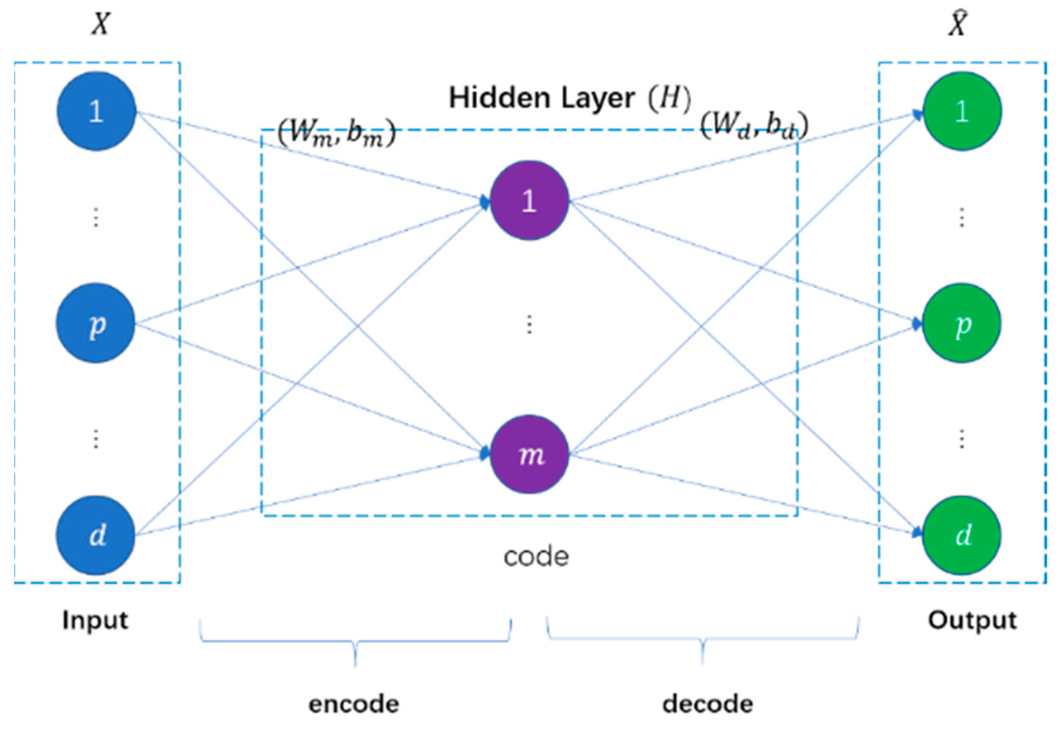
Like most unsupervised deep learning models, the auto-encoder seeks to achieve abstract learning of input samples by equating the network’s predicted output with the input samples. Rumelhart et al. [21] suggested the auto-encoder concept first, and then Bourlard et al. [22] discussed it. An encoder and a decoder are generally found in an auto-encoder. The encoder translates high-dimensional input samples to low-dimensional abstract representations to minimize sample dimensionality. The decoder translates the abstract representations into predicted outputs to replicate the input samples. It adjusts the network parameters to minimize the reconstruction error to acquire the best abstract representation of the input samples. Figure 3 depicts the auto-encoder structure.
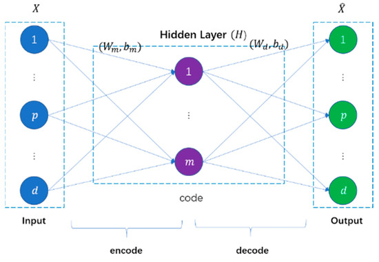
Figure 3.
Auto-encoder structure.
Suppose given an input sample , where represents the dimension of the input sample and is the number of input samples. The weight matrix and bias of the encoder and decoder are , and , , respectively. is the activation function of each layer. The auto-encoder sends samples to the encoder and uses linear mapping and a nonlinear activation function to finish the encoding.
The decoder then completes the decoding of the encoded features. It obtains the input sample reconstruction . Given the encoding , can be thought of as a prediction of with the same dimension as . The decoding procedure is similar to that of encoding.
The L2 loss is commonly employed as a cost function for reconstruction to optimize the weight matrix and biases parameters. It can be stated as follows:
To learn feature representations in the sample data, auto-encoders commonly use a gradient descent technique to backpropagate the error to alter the network parameters and gradually reduce the reconstructed error function by iterative fine-tuning. Assuming that the learning rate is , the auto-connection encoder’s weights and bias update formulas are as follows:
Figure 4 shows how this paper extracts characteristics from response data using a deep auto-encoder with five hidden layers. Deep auto-encoders with multiple hidden layers can learn more complex underlying feature representations of input data mathematically than auto-encoders with only one hidden layer. The encoder is represented by layers to , while layers to represent the decoder in Figure 4. The previous layer’s output is used as the next layer’s input. The encoder weight matrices , and are used to learn the final compressed feature representation on the layer; , , and are the encoder biases. The decoding matrices , , and the biases , , of the decoder are responsible for reconstructing input data on output layer using the learned feature representation on the layer. The function aims to strengthen the learning ability of the auto-encoder. In this paper, the autoencoder adopts Equation (3) as the reconstruction loss function. When the undamaged data is input, the reconstruction loss will be slight; when the damaged data is input, the reconstruction loss is often much more significant than when the undamaged data is input.
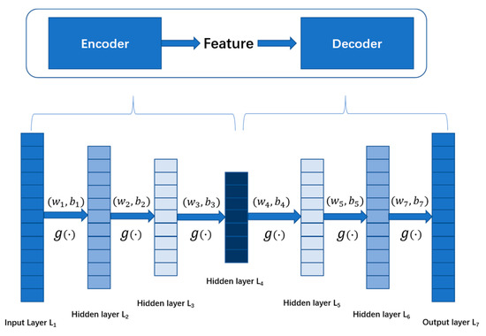
Figure 4.
The structure of the auto-encoder in this paper.
2.1.2. Introducing the Score-Guided Regularization Strategy to Expand Anomaly Score Differences
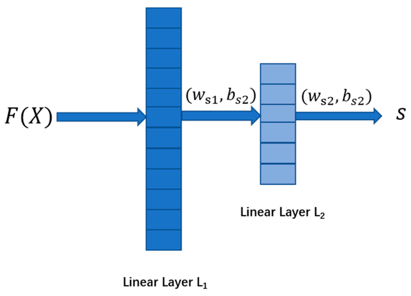
Specifically, the score-guided regularization strategy [23] extracts valuable information from ostensibly undamaged and damaged samples, with more miniature scores for undamaged samples and higher scores for damaged samples. Making full use of apparent data enhances representation learners’ optimization, leading undamaged and damaged samples in different directions. Furthermore, the score-guided network directly learns discriminative metrics. It has more robust capabilities because it provides anomaly scores end-to-end rather than relying on pre-defined distance metrics or reconstruction errors. Figure 5 depicts the score-guided network structure of this article. The function is a pre-defined d function used to learn the data’s features. In this model, the pre-defined d function refers to the auto-encoder, represents the training data, and represents the abstract representations of . The score-guided network in this paper only contains two linear layers and , which are used to convert the learned latent features into scores . and are the weight matrix and bias of the two linear layers, respectively.

Figure 5.
The score-guided network structure of this paper.
The loss function of the score-guided network is defined as follows:
where is the threshold, after processing by the pre-defined d function , if it is lower than ε, we consider the current sample to be an apparent undamaged sample; otherwise, we consider the current sample to be a suspicious damaged sample. Parameter determines the guiding position of an anomaly score; and are used as weight parameters to adjust the guiding effect of the anomaly score. We set a very small positive value approaching 0 to be the target anomaly scores for the apparent undamaged data, due to that the zero scores will force most weights of the score-guided network to be 0.
Since refers to the auto-encoder in this paper, we can take the reconstruction error of the auto-encoder as a self-supervised signal. We take the loss function of the auto-encoder (Equation (3)) as . Therefore, the above loss function expression can be written as:
From another perspective, the regularization function can be rewritten as follows:
is the undamaged data part, and is the suspected damaged part.
It’s worth mentioning that a large , intuitively, can better enlarge the score gap between the undamaged and damaged data. However, a too large will only lengthen the distribution of scores, and the performance improvement will stabilize with the increase of . As the score-guided network learns the anomaly score and determines the effect together with , the actual impact of is small, not requiring adjustment; therefore, we set in all experiments.
2.1.3. Tuning Parameters Using Multi-Task Learning
Multi-task learning is a technique for optimizing multi-objective models employed in many deep learning tasks [24]. Multi-task learning tries to enhance learning efficiency and prediction accuracy by learning numerous targets from a joint representation instead of constructing a separate model for each task [25]. It can be thought of as a way to increase inductive knowledge transfer by allowing complementary tasks to share domain information. The auto-encoder task and the score-guided network task are two subtasks of the approach provided in this paper. The loss functions of the auto-encoder and the score-guided network are and , respectively, according to Equations (3) and (7).
In multi-task learning, the optimal training effect can only be achieved by weighting the loss function of the subtasks appropriately. The loss function of the algorithm in this paper adopts the typical loss function expression as follows:
where is the weights of the loss function of the auto-encoder; is the weights of the loss function of the score-guided network. The model’s performance depends heavily on the choice of these two parameters. We introduce uncertainty to determine these two parameters [26] automatically. The core idea of this method is to give lower loss function weights to tasks with higher uncertainty to reduce the difficulty of training.
This strategy is based on a Bayesian model that includes two types of uncertainty: Epistemic uncertainty and Aleatoric uncertainty. Epistemic uncertainty is a type of model uncertainty that describes what our model does not know owing to a lack of training data. Our uncertainty about information that our data cannot explain is captured by Aleatoric uncertainty. There are two types of Aleatoric uncertainty: data-dependent uncertainty and task-dependent uncertainty. Data-dependent uncertainty is expected as a model output and is dependent on the input data. Task-dependent uncertainty is not dependent on the input data. It is not a model output; instead, it is a quantity that stays constant for all input data and varies between different tasks. Task-dependent uncertainty measures the relative confidence between tasks in a multi-task environment, representing the uncertainty inherent in the regression or classification task. Hence, we use task-dependent uncertainty as the basis for weighted loss.
After introducing noise (uncertainty) parameters and for auto-encoder and score-guided networks. The final loss function of the proposed model is:
We can see that as the noise continues to increase, the task’s weight decreases. is the standard term of this loss function, which aims to prevent a certain from being too large and causing serious imbalance in model training. Parameters and are optimized by the back error propagation algorithm.
2.1.4. Data Generation
Consider a structure equipped with joints (or accelerometers). A total of experiments are carried out to construct the training data set. The first experiment () involves measuring acceleration signals across the entire structure. In the remaining experiments, each experiment has one joint damaged. For the data collected by each accelerometer, we can divide it into damaged data and undamaged data, as follows:
where and indicate the measurements acquired for the damaged and undamaged structural cases, respectively. represents the data obtained by the th accelerometer in the th experiment. We can notice that the undamaged data set for the th joint includes signals measured when all joints are undamaged () and signals measured when one of the other joints is damaged. The purpose of this is to eliminate the mutual influence between joints.
The next step is to normalize the data. To be more realistic, we do not normalize the damaged and undamaged data separately, which most current studies use, but normalize the damaged and undamaged data together. The normalization process is expressed as follows:
where is the vectors after uniform standardization, and represents the normalization function. and represent damaged and undamaged vectors in , respectively. The next step is to partition the undamaged and damaged vectors into many frames, each with a fixed number() of samples. This operation’s outcome for joint can be written as:
where and are vectors containing the damaged and undamaged frames for the joint , respectively. and are the total number of damaged and undamaged frames, respectively. Given the total number of samples in each acceleration signal ; and can be computed as:
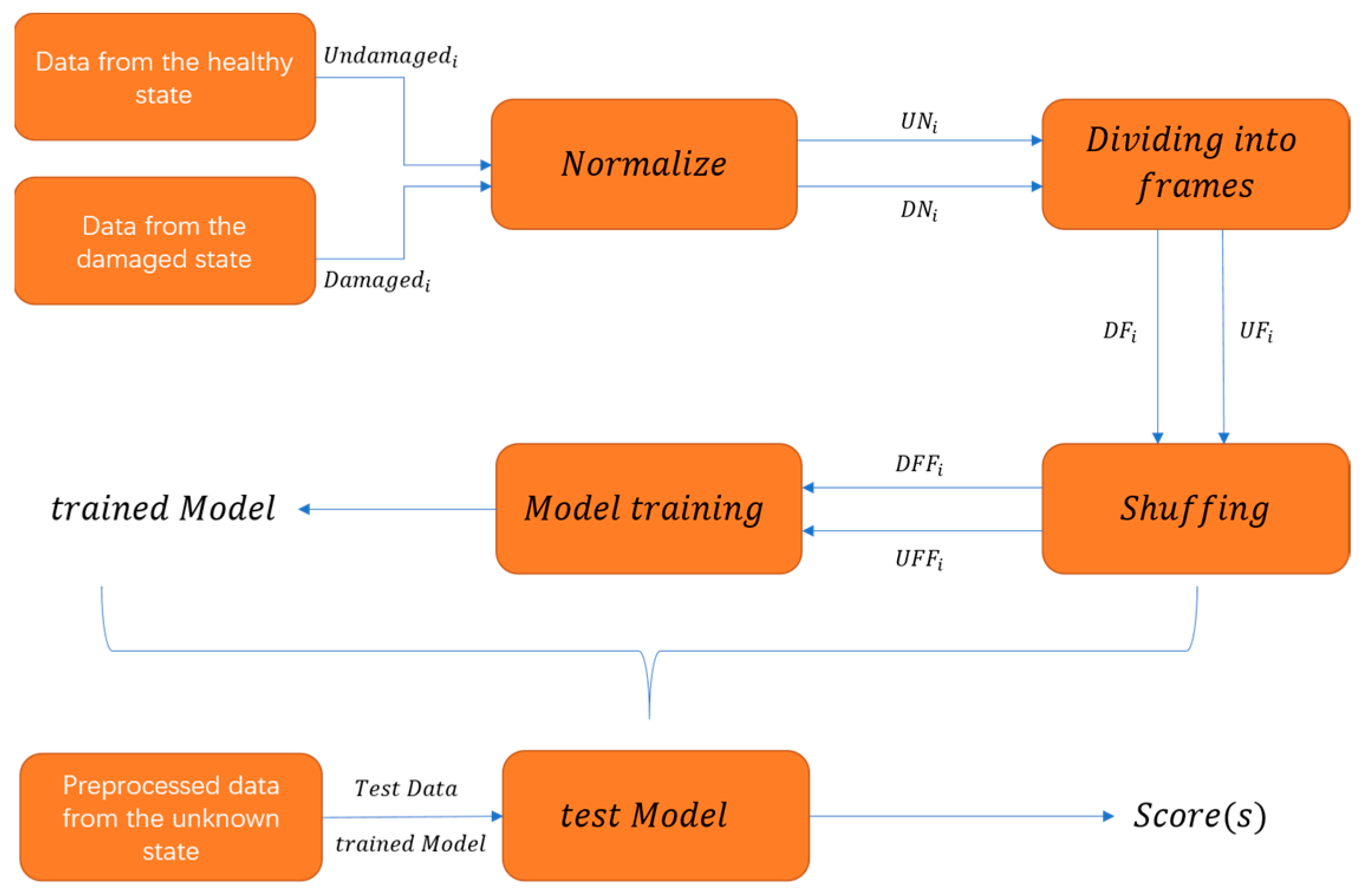
It is clear from Equations (20) and (21) that the number of undamaged frames will be much greater than the number of damaged frames for a given joint . Some researchers choose the same amount of damaged and undamaged frames for training to avoid the impact of imbalance on performance, which is impracticable. As a result, selecting the same number of damaged and undamaged frames is skipped. Then, send the damaged and undamaged frames to train in a jumble. Figure 6 depicts the specific flow chart. After the data has been processed, it is fed into the model for training, and a trained model is generated. After processing data from an unknown state according to the previous stages, input it into the trained model for testing. Finally, the model generates a score , representing the current data’s damage score.
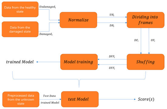
Figure 6.
The brief flow of the model from data processing to training model to testing.
2.2. Algorithm
Algorithm 1 illustrates the proposed algorithm’s process., and represent the encoder, decoder and score-guided network, respectively; and are the noise parameters of the auto-encoder and score-guided network. These parameters are initialized randomly and optimized in the training iteration (Steps 3–13) to minimize the loss in Equation (10). Specifically, the representation learner learns the data representation Z through in Step 6. Then, the scoring network learns the anomaly scores s through in Step 8. Then, Step 9 calculates the loss function, and Steps 10 and 11 take a backpropagation algorithm and update the network parameters. Data representation and anomaly score distribution are optimized during training. Given a trained model, anomaly scores can be directly calculated given new data samples.
| Algorithm 1. |
| Input: , Output: |
, |
3. Experiment
3.1. Verification on the Qatar University Grandstand Simulator
This section uses the QU grandstand simulator (QUGS) [27] to verify the proposed damage detection algorithm.
3.1.1. Qatar University Grandstand Simulator
A total of 30 spectators can be accommodated in the QU grandstand simulator. As shown in Figure 7, the steel frame comprises 8 major girders and 25 filler beams supported by 4 columns. The 8 girders are 4.6 m long, while the 5 filler beams in the cantilevered area are around 1 m-long and the remaining 20 beams are each 77 cm long. The two long columns are approximately 1.65 m long. The grandstand simulator’s primary steel frame has 30 accelerometers installed on the major girders at the 30 joints. For more detail on the structure, the readers are directed to [27].
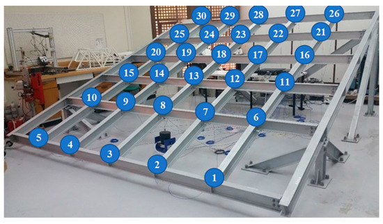
Figure 7.
The main steel frame of the QU grandstand simulator [27].
3.1.2. Experiment Setup
To obtain the training data set, researchers did 31 experiments [27]. The first experiment was carried out under the entire case, whereas the others were carried out under damaged cases caused by loosening one or more of the 30 beam-to-girder joints. Following Section 2.1.4, the frame length was taken as 128 samples after standardization; hence, vectors and contain 63,488 frames for each joint where and . Only 20% of these frames were used for the testing process, 72% for the training process, and 8% for validation. Therefore, the length of the training set, validation set, and test set are 45,711, 5079, and 12,698, respectively. The model is trained using forward and backpropagation after the processed data has been shuffled.
As illustrated in Figure 4, a deep auto-encoder with seven layers was used. In each test, the size of the deep auto-input encoder’s layer was equal to the length of the collected acceleration data. Layers through in Figure 4 have sizes of 128, 80, 40, 20, 40, 80, and 128, respectively. The score-guided network comprises two linear layers with sizes of 20 and 10 units each. The batch size in each experiment is 1024, the training epochs are 100, and the Adam optimizer’s learning rate is 0.0001. Table 1 shows the anomaly scores for 30 accelerometers. All experiments were performed 5 times.

Table 1.
Mean anomaly scores of undamaged and damaged data. ID column represents the code of the accelerometer; the Undamaged column represents the average anomaly score of the undamaged data; and the Damaged column represents the anomaly score of the damaged data.
3.1.3. Discussions
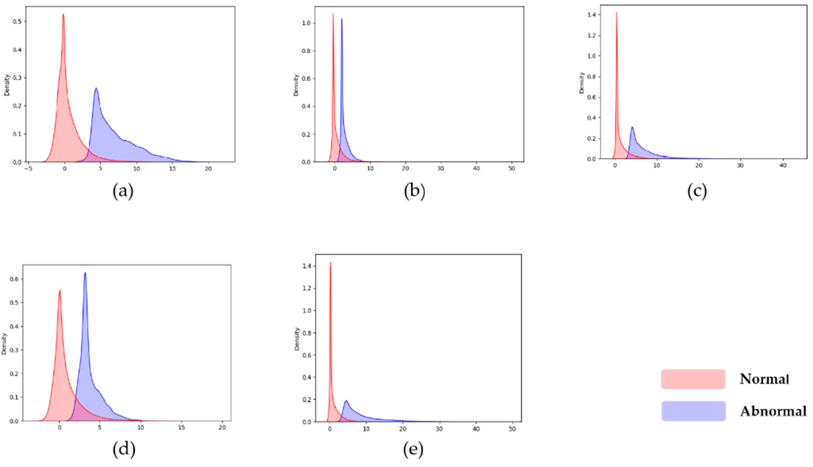
The scores of the trained models on the test sets are shown in Table 1. The ID column is the accelerometer’s code; the Undamaged and Damaged column is the average anomaly score of the undamaged and damaged data. As indicated in Table 1, the anomaly scores for the undamaged and damaged data can be separated for most accelerometers. Damaged data can be distinguished from undamaged data if an appropriate strategy for selecting an anomaly score threshold is used. The first accelerometer, for example, has an average anomaly score of 0.384 for undamaged data and a value of 5.784 for damaged data, indicating good discrimination. We draw the score distribution density map of the first five accelerometers in Figure 8 to examine the score distribution quickly. The x-axis represents the score, and the y-axis represents the density of the score; (a) to (e) are the score distribution density maps of accelerometers 1 to 5. The undamaged and damaged data scores are greatly staggered in the score distribution displayed in Figure 8, indicating that our model successfully enhances the gap between the undamaged and damaged data.
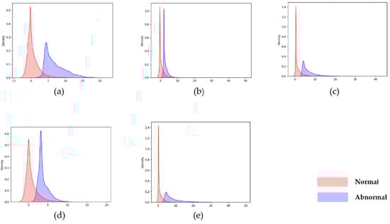
Figure 8.
Score distribution of the first five accelerometers, the x-axis represents the score, and the y-axis represents the density of the score distribution. (a–e) represent accelerometer 1 to 5.
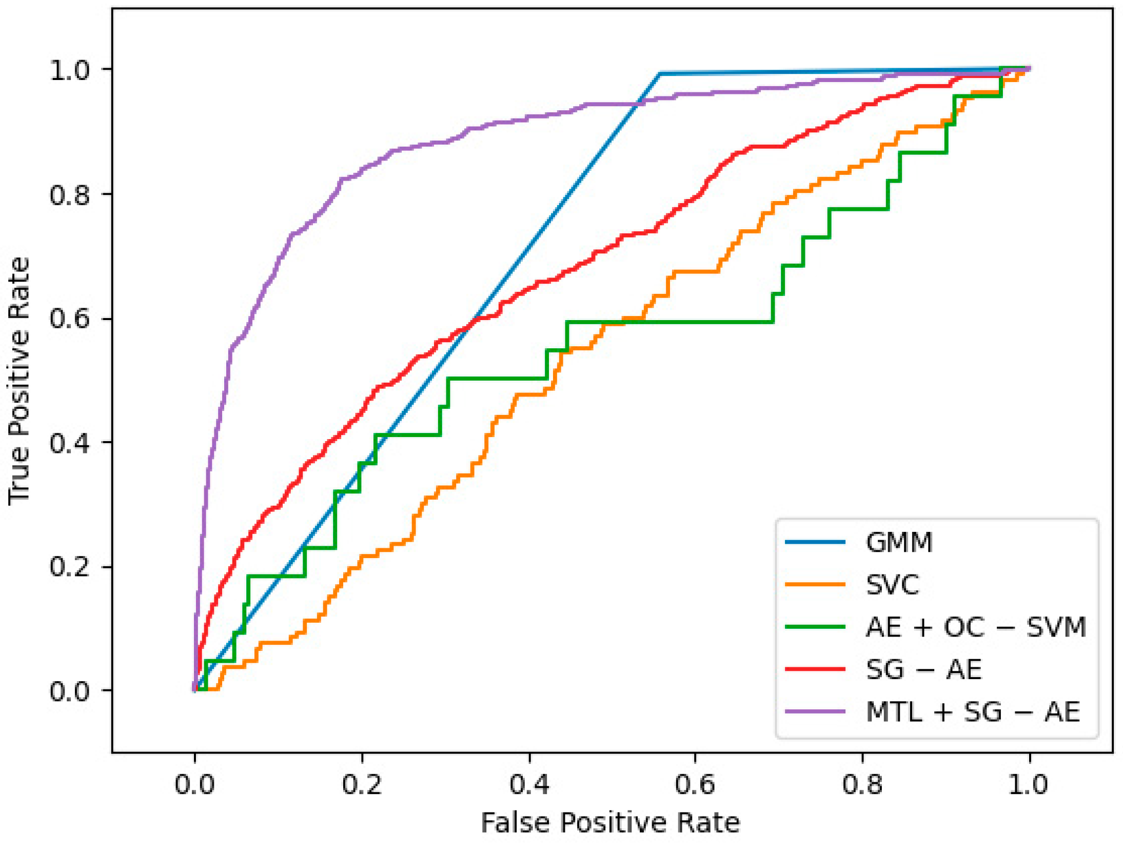
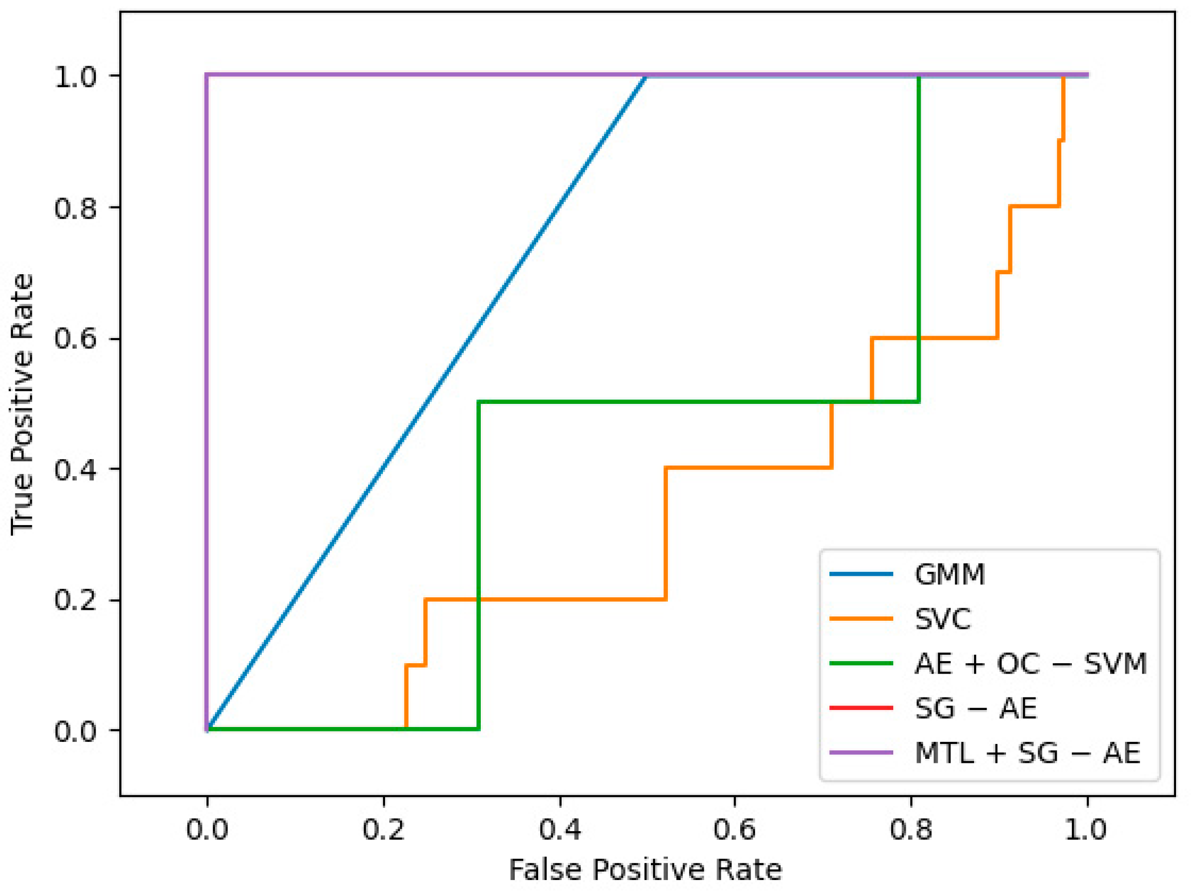
The ROC-AUC is used as a measurement indicator to evaluate our algorithm’s (replaced by MTL + SG − AE below) performance. The ROC curve depicts the relative trade-off between true positive (TP) and false positive (FP) probabilities, where TP refers to the probability of judging undamaged samples as undamaged samples, and FP refers to the probability of judging damaged samples as undamaged samples [28]. In the process of choosing comparison algorithms, we found that cluster-based methods account for a large proportion of unsupervised structural damage detection, so we chose two classic cluster-based unsupervised methods as comparison algorithms: Gaussian Mixture Model (GMM) and Support Vector Clustering (SVC). At the same time, we noticed that the combination of autoencoder and traditional algorithm has also become a trend of unsupervised structural damage detection, so we also use the algorithm combining autoencoder and one-class support vector machine(AE + OC − SVM) as one of the comparison algorithms. Finally, to demonstrate the effectiveness of multi-task learning, we also incorporate the algorithm (SG − AE) without introducing it as our comparative experiment.
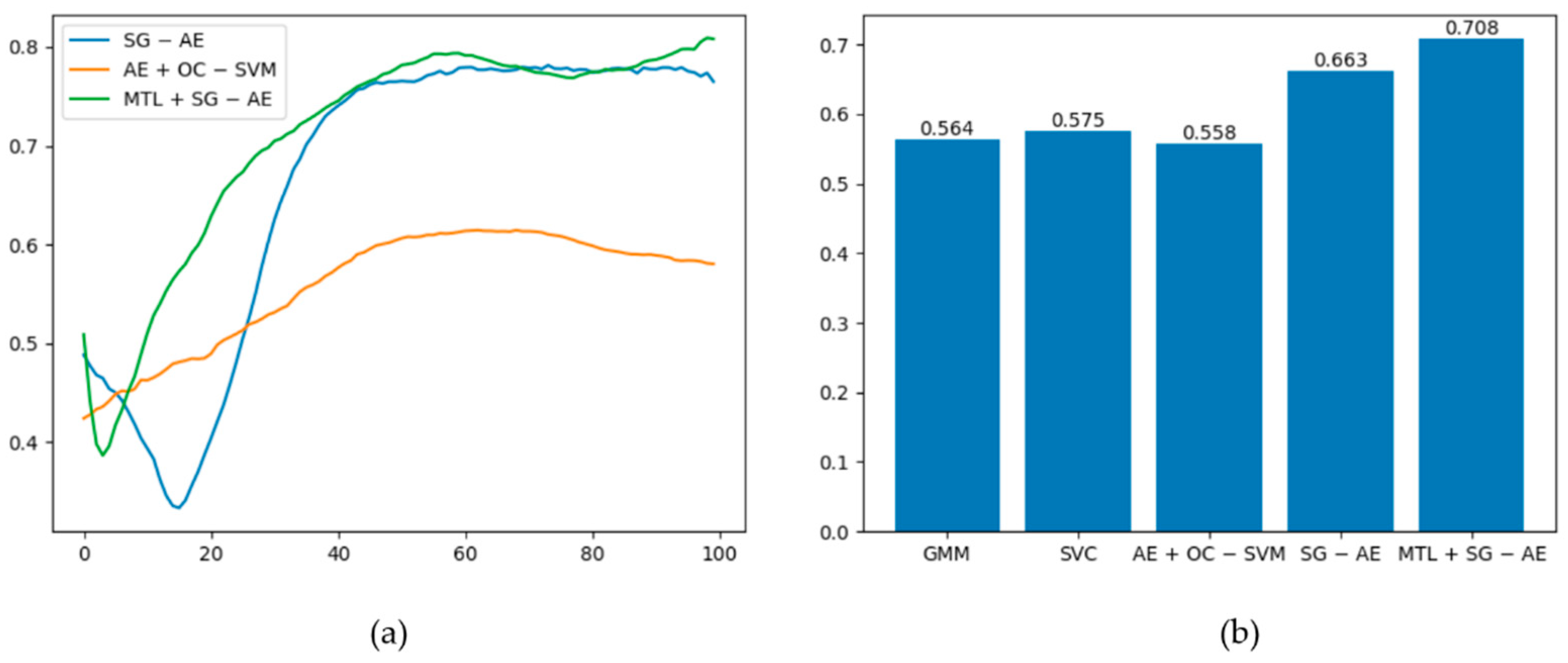
The best ROC curves of the five methods under this dataset are plotted in Figure 9, and the graph demonstrates that MTL + SG − AE has the maximum area under the curve (AUC). Among the five algorithms, only AE + OC − SVM, SG − AE, and MTL + SG − AE are deep algorithms. Figure 10a shows the AUC values of these three algorithms changes with the training epochs. Figure 10a shows that the performances of SG − AE and MTL + SG − AE are significantly better than that of AE + OC − SVM; additionally, the multi-task learning we implemented improves the performance of MTL + SG − AE over that of SG − AE. The mean AUC of the five algorithms is shown in Figure 10b. As can be shown, the average AUC of all algorithms is more than 0.5, implying that these algorithms have unique effects on this dataset. MTL + SG − AE, on the other hand, has the highest average AUC of 0.708.

Figure 9.
The best ROC curves of five algorithms.
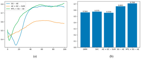
Figure 10.
(a) Graph of the AUC values of the three depth algorithms changing with the training epochs. (b) Average AUC of the five algorithms.
3.2. Verification on Experimental Phase II of the SHM Benchmark Data
The study presented in this section is based on experimental phase II of the SHM benchmark problem data [29].
3.2.1. Experimental Phase II of the SHM Benchmark Data
The International Association for Structural Control (IASC)—American Society of Civil Engineers (ASCE) Structural Health Monitoring Task Group published the data in 2003 as a benchmark. A four-story steel structure developed at the University of British Columbia serves as the benchmark frame. The structure was fitted with fifteen accelerometers. For more information on the laboratory structure, the readers are directed to [29]. On the benchmark frame, nine structural damage situations were simulated. Under ambient stimulation, 15 accelerometers measured acceleration output for each case. As illustrated in Table 2, structural damage progressed from undamaged (Case 1) to severely damaged (Case 9).
Table 2.
Description of the structural cases in the benchmark problem.
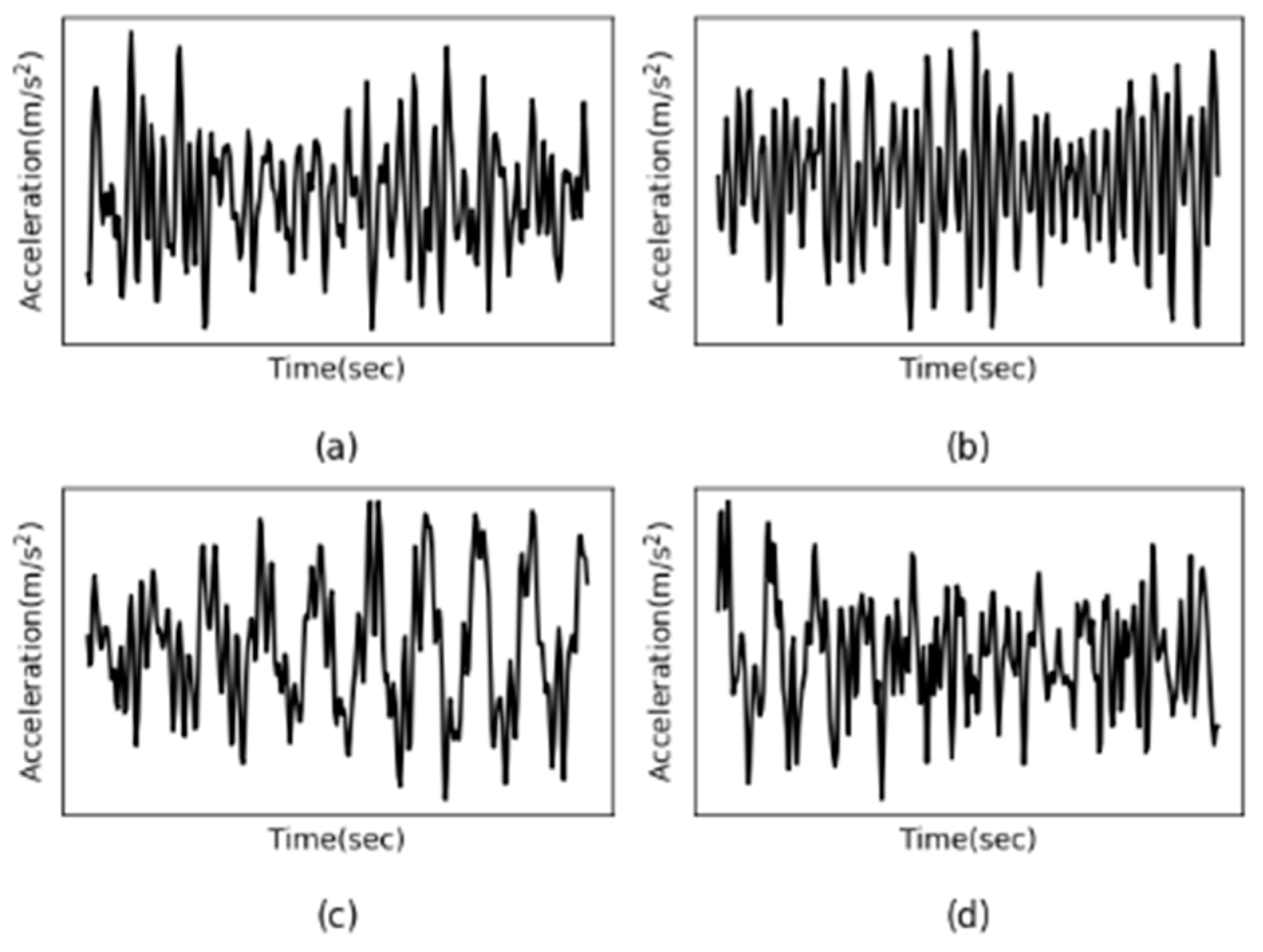
It should be noted that vibration data from accelerometers 1 to 3 mounted on the structural ground was ignored due to insufficient power and information [30]. Therefore, the vibration signal of accelerometers 4 to 15 is analyzed in this paper. Due to the importance of the nature of vibrational signals, some signals are visualized to assess their nature. For example, Figure 11 shows the acceleration measurement history of the 10th accelerometer from Case 1 to Case 4, with (a) to (d) representing Case 1 to Case 4. As can be seen from the graph below, the vibrational response of the 10th accelerometer due to ambient vibrations appears to be non-stationary. More precisely, Entezami et al. [31] showed that most of the vibration signals of ASCE structures have non-stationary behavior.

Figure 11.
The acceleration response of the 10th accelerometer from Case 1 to 4. (a–d) represent Case 1 to 4.
3.2.2. Experiment Setup
As previously stated, 12 accelerometers were employed in training. From [29], we can know that the acceleration measurements were captured at 200 Hz in all cases. The vibration response was measured for 300 s in Cases 1 through 5, 227.84 s in Case 6, and 900 s in the other cases.
The data gathered for the whole structure (Case 1) and the data collected while the structure was severely damaged (Case 9) were used for training in this experiment. Following Section 2.1.4, using samples as the frame length, each of Case 1’s 12 undamaged signals was divided into frames, while Case 9’s 12 entirely damaged signals were separated into frames. Overall, 70% of the data should be used for training and 30% for testing, and 328 healthy samples and 983 damaged samples were used for training for each accelerometer. The model configuration of this experiment is the same as the model configuration in Section 3.1.2.
To test the trained model and reflect the health status of the structure more intuitively, the data collected in 9 cases is decomposed into samples according to Section 2.1.4, then input processed data to the corresponding trained model. The model will output an anomaly score for the current sample, reflecting the likelihood of damage to the entire structure. Anomaly scores for all cases are shown in Table 3. All experiments were performed 5 times.
Table 3.
Anomaly scores of 12 accelerometers in 9 cases.
3.2.3. Discussions
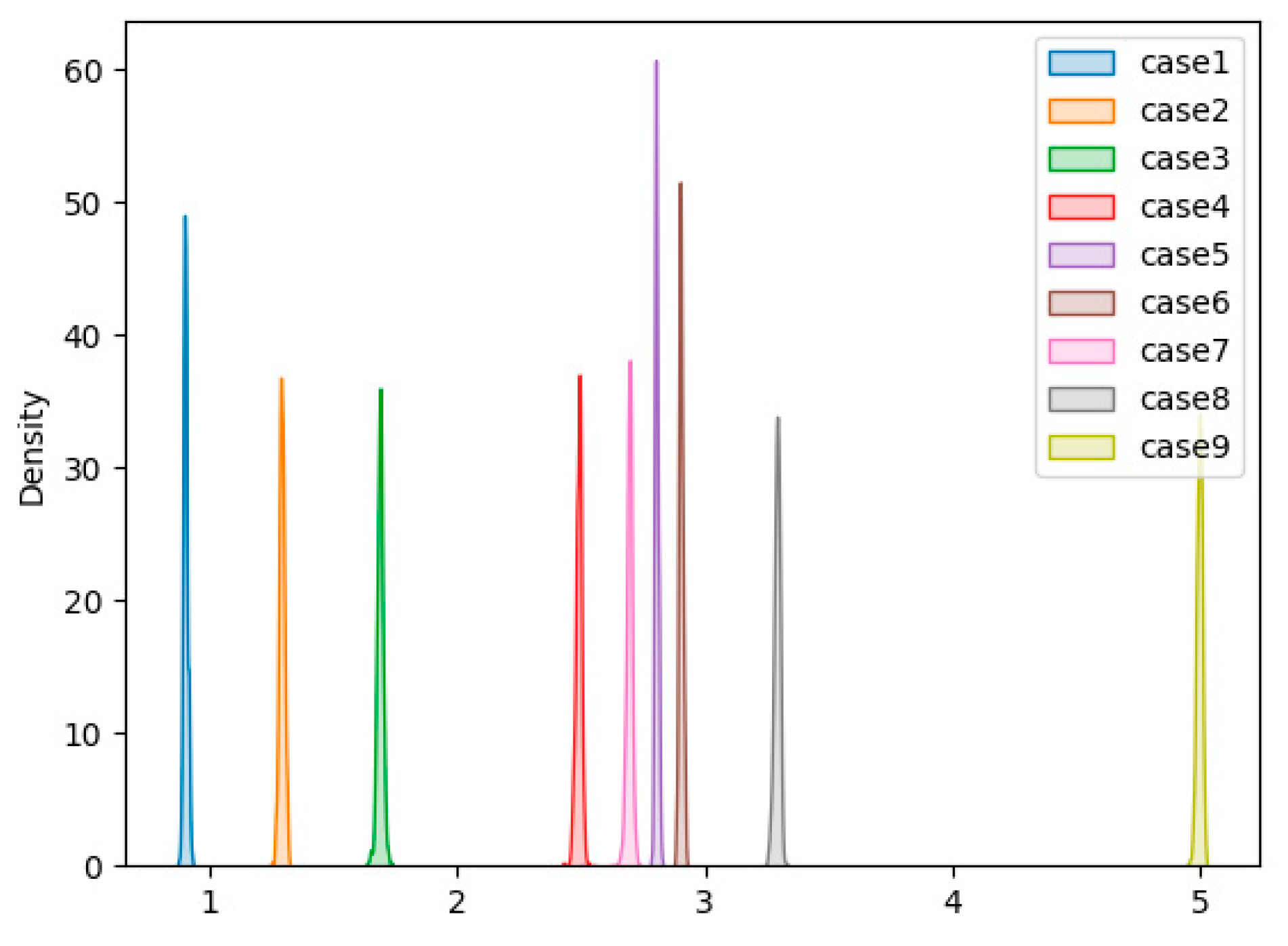
The experimental results are shown in Table 3. As far as the entire structure is concerned, with the increase in the overall damage degree of the structure, the mean anomaly score shows a steady upward trend. For the undamaged case (Case 1), the average anomaly score is 0.824, the lowest average anomaly score compared to the average anomaly scores in the other cases, indicating that the current situation has the lowest probability of overall structural stability damage. In Case 2, removing a single diagonal brace increased the value to 1.115. When additional braces were removed in Cases 3–6, the average anomaly scores gradually climbed from 1.298 in Case 3 to 1.792 in Case 6. In Case 7, however, when all of the remaining diagonal braces were eliminated, the anomaly score jumped to 2.118. Finally, the anomaly score has grown to 3.655 due to loosened bolts in Cases 8 and 9, revealing a significant gap inside the entire structure. As far as a single sensor is concerned, it can be observed that the proposed algorithm exhibits remarkable results on most accelerometers. As the damage degree increases, the anomaly score also increases. In Case 9, most anomaly scores are more extensive than 4, and the anomaly scores of some accelerometers are even more significant than 5, gradually approaching 6. Figure 12 has drawn the score distribution of the 1st accelerometer in 9 cases. The figure shows that as the degree of damage increases, the anomaly score becomes larger and larger, and there are clear boundaries between the different degrees of damage.
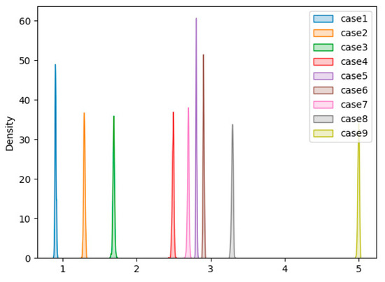
Figure 12.
Score density plot of the 1st accelerometer in 9 cases.
Interestingly, the trained model can also better detect the degree of structural damage in the remaining cases, despite only using a portion of the data from Cases 1 and 9. In other words, even though the acceleration signals in Cases 2–8 and the remaining frames in Cases 1 and 9 were unfamiliar to the algorithm, it was able to assign a good anomaly score that accurately reflected the actual degree of damage in all cases.
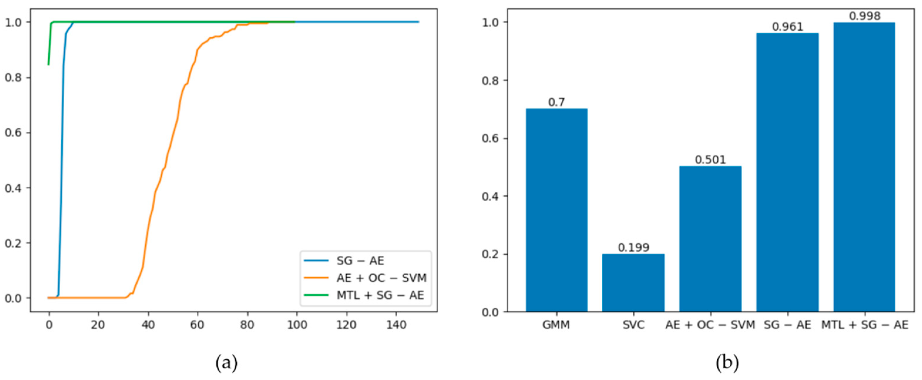
We also compare our proposed method with the four algorithms mentioned in Section 3.1.3. Figure 13 shows the best ROC curves of the five algorithms; in this figure, the ROC curves of SG − AE and MTL + SG − AE overlap, and the AUC values are both 1. According to [28], we know that when the value of AUC is 1, the model is perfect. Therefore, these two algorithms are perfect for this dataset. Figure 14a shows the variation trends of the AUC values of the three depth algorithms during training. It is not difficult to find that the final AUC values are all 1, but during the training process, the initial AUC value of MTL + SG − AE is 0.8, while the other two algorithms are 0. Compared with the other two algorithms, MTL + SG − AE has a faster speed converging to 1, reflecting the algorithm’s excellent training. Figure 14b depicts the average AUC of the five algorithms. The figure shows that the performance of MTL + SG − AE is much better than that of GMM, SVC, AE + OC − SVM. Moreover, compared with SG − AE, the average AUC is also improved from 0.961 to 0.998, which shows the effectiveness of multi-task learning.
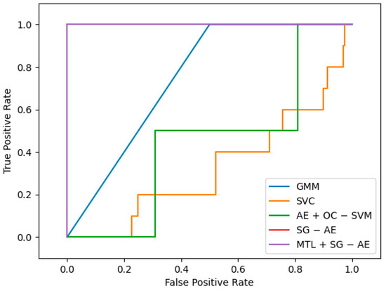
Figure 13.
The best ROC curves of the five algorithms, in which the curve of SG − AE coincides with the curve of MTL + SG − AE.
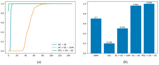
Figure 14.
(a) Graph of the AUC values of the three depth algorithms changing with the training epochs; (b) Average AUC of the five algorithms.
To make the claims more substantiated, we also compared with other method using SHM benchmark data. Literature [5] used SHM benchmark data to verify the performance of the proposed unsupervised method, this method utilizes the distribution of the PoD values throughout the structure to identify the location of structural damage will be investigated. In their study, Case 1 has the smallest value of PoD and the Case 9 has the biggest value of PoD, which is similar to the distribution of anomaly score under this dataset. However, they only use undamaged data for training, and do not take into account that it is difficult to ensure the acquired data is completely undamaged in actual cases. These methods can provide judgment support for decision makers, but our algorithm is more suitable for practical scenarios and can be more flexibly integrated into other damage detection frameworks.
4. Conclusions
This study proposes a new unsupervised machine learning-based structural damage detection method. The biggest difference from other unsupervised methods is the use of contaminated data for training, which makes the model more suitable for actual structural monitoring scenarios. In particular, proposed method is composed by: (1) auto-encoder, which is used to extract the features of the sample; (2) score-guided regularization network, which is used to expand the abnormal score difference between healthy samples and damaged samples, so that the model can learn more representational information. Specifically, it is to make full use of obvious data to enhance the optimization of representation learners, so that samples with small damage can also be given larger abnormal scores; (3) multi-task learning, which simplifies the parameter tuning process of the model by introducing uncertain parameters. After a detailed description of each phase, we validated the performance on the QUGS and ASCE (II). Experimental results show that the proposed method achieves good results on both the above datasets, providing reliable estimates for structural damage detection.
For concluding, we wish to highlight a proposed method that can be applied in many structural damage monitoring scenarios to develop risk mitigation strategies:
- (1)
- The proposed method generates a separate model for each monitoring point, so even if there are few monitoring points available in the real-case structure monitoring, the method can be well applied.
- (2)
- The proposed method outputs anomaly scores in an end-to-end manner without requiring prior knowledge to define various indicators in advance, making the model more convenient to apply to different scenarios.
- (3)
- The proposed method uses contaminated data for training, which is more suitable for actual structural monitoring scenarios and provides higher applicability.
Although the suggested unsupervised method performs well in detecting structural damage, how to define a score threshold based on the output anomaly score is still a challenge, which is also one of the challenges of unsupervised learning. Some variant algorithms based on extreme value theory are worthy of consideration to deal with the problem of threshold estimation.
Author Contributions
Conceptualization, Y.Q.; methodology, Y.Q.; software, Y.Q.; validation, Y.Q.; formal analysis, Y.Q. and S.Z.; investigation, Y.Q.; resources, Y.Q. and K.C.; data curation, Y.Q.; writing—original draft preparation, Y.Q.; writing—review and editing, Y.Q. and S.Z.; visualization, Y.Q.; supervision, S.Z.; project administration, Y.Q. All authors have read and agreed to the published version of the manuscript.
Funding
This research received no external funding.
Institutional Review Board Statement
Not applicable.
Informed Consent Statement
Not applicable.
Data Availability Statement
Not applicable.
Conflicts of Interest
The authors declare no conflict of interest.
References
- Farrar, C.R.; Worden, K. Structural Health Monitoring: A Machine Learning Perspective, 1st ed.; John Wiley & Sons: Chichester, UK, 2012; pp. 16–239. [Google Scholar]
- Barthorpe, R.J. On Model- and Data-Based Approaches to Structural Health Monitoring. Ph.D. Thesis, University of Sheffield, Sheffield, UK, 2014. [Google Scholar]
- Alcover, I.F. Data-Based Models for Assessment and Life Prediction of Monitored Civil Infrastructure Assets. Ph.D. Thesis, University of Surrey, Guildford, UK, 2014. [Google Scholar]
- Mohsen, A.; Armin, D.E.; Gokhan, P. Data-driven structural health monitoring and damage detection through deep learning: State-of-the-art review. Sensors 2020, 20, 2778. [Google Scholar]
- Abdeljaber, O.; Avci, O.; Kiranyaz, M.S.; Boashash, B.; Sodano, H.; Inman, D.J. 1-D CNNs for structural damage detection: Verification on a structural health monitoring benchmark data. Neurocomputing 2018, 275, 1308–1317. [Google Scholar] [CrossRef]
- Avci, O.; Abdeljaber, O.; Kiranyaz, M.S.; Inman, D. Structural Damage Detection in Real Time: Implementation of 1D Convolutional Neural Networks for SHM Applications. In Structural Health Monitoring & Damage Detection, 7th ed.; Springer: Berlin, Germany, 2017; pp. 49–54. [Google Scholar]
- Sergio, R.; Angelo, C.; Valeria, L.; Uva, G. Machine-learning based vulnerability analysis of existing buildings. Autom. Constr. 2021, 132, 103936. [Google Scholar]
- Sanayei, M.; Khaloo, A.; Gul, M.; Catbas, F.N. Automated finite element model updating of a scale bridge model using measured static and modal test data. Eng. Struct. 2015, 102, 66–79. [Google Scholar] [CrossRef]
- Ding, X.M.; Li, Y.H.; Belatreche, A.; Maguire, L. An experimental evaluation of novelty detection methods. Neurocomputing 2014, 135, 313–327. [Google Scholar] [CrossRef]
- Sarmadi, H.; Karamodin, A. A novel anomaly detection method based on adaptive Mahalanobis-squared distance and one-class kNN rule for structural health monitoring under environmental effects. Mech. Syst. Signal Process. 2019, 140, 106495. [Google Scholar] [CrossRef]
- Da Silva, S.; Júnior, M.D.; Junior, V.L.; Brennan, M.J. Structural damage detection by fuzzy clustering. Mech. Syst. Signal Process. 2008, 22, 1636–1649. [Google Scholar] [CrossRef]
- Rafiei, M.H.; Adeli, H. A novel unsupervised deep learning model for global and local health condition assessment of structures. Eng. Struct. 2018, 156, 598–607. [Google Scholar] [CrossRef]
- Long, J.; Buyukozturk, O. Automated structural damage detection using one-class machine learning. In Dynamics of Civil Structures, 4th ed; Springer: Cham, Germany, 2014; pp. 117–128. [Google Scholar]
- Wang, Z.; Cha, Y.J. Unsupervised deep learning approach using a deep auto-encoder with a one-class support vector machine to detect structural damage. Struct. Health Monit. 2020, 20, 406–425. [Google Scholar] [CrossRef]
- Diez, A.; Khoa, N.L.D.; Alamdari, M.M.; Wang, Y.; Chen, F.; Runcie, P. A clustering approach for structural health monitoring on bridges. J. Civ. Struct. Health Monit. 2016, 6, 429–445. [Google Scholar] [CrossRef] [Green Version]
- Cha, Y.-J.; Wang, Z.L. Unsupervised novelty detection–based structural damage localization using a density peaks-based fast clustering algorithm. Struct. Health Monit. 2017, 17, 313–324. [Google Scholar] [CrossRef]
- Fan, W.; Qiao, P. Vibration-based Damage Identification Methods: A Review and Comparative Study. Struct. Health Monit. 2011, 10, 83–111. [Google Scholar] [CrossRef]
- Cao, M.S.; Sha, G.G.; Gao, Y.F.; Ostachowicz, W. Structural damage identification using damping: A compendium of uses and features. Smart Mater. Struct. 2017, 26, 043001. [Google Scholar] [CrossRef]
- Barman, S.; Mishra, M.; Maiti, D.; Maity, D. Vibration-based damage detection of structures employing Bayesian data fusion coupled with TLBO optimization algorithm. Struct. Multidiscip. Optim. 2021, 64, 2243–2266. [Google Scholar] [CrossRef]
- Pathirage, C.S.N.; Li, J.; Li, L.; Hao, H.; Liu, W.; Ni, P. Structural damage identification based on autoencoder neural networks and deeplearning. Eng. Struct. 2018, 172, 13–28. [Google Scholar] [CrossRef]
- Rumelhart, D.E.; Hinton, G.E.; Williams, R.J. Learning representations by back-propagating errors. Nature 1986, 323, 533–536. [Google Scholar] [CrossRef]
- Bourlard, H.; Kamp, Y. Auto-association by multilayer perceptrons and singular value decomposition. Biol. Cybern. 1988, 59, 291–294. [Google Scholar] [CrossRef]
- Huang, Z.Y.; Zhang, B.H.; Hu, G.Q.; Li, L.; Xu, Y.; Jin, Y. Enhancing Unsupervised Anomaly Detection with Score-Guided Network. arXiv 2021, arXiv:2109.04684. [Google Scholar]
- Caruana, R. Multitask learning. Mach. Learn. 1997, 28, 41–75. [Google Scholar] [CrossRef]
- Baxter, J. A model of inductive bias learning. J. Artif. Intell. Res. 2000, 12, 149–198. [Google Scholar] [CrossRef]
- Cipolla, R.; Gal, Y.; Kendall, A. Multi-task Learning Using Uncertainty to Weigh Losses for Scene Geometry and Semantics. In Proceedings of the 2018 IEEE/CVF Conference on Computer Vision and Pattern Recognition, Salt Lake City, UT, USA, 18–23 June 2018; pp. 7482–7491. [Google Scholar]
- Abdeljaber, O.; Avci, O.; Kiranyaz, S.; Gabbouj, M.; Inman, D.J. Real-time vibration-based structural damage detection using one-dimensional convolutional neural networks. J. Sound Vib. 2017, 388, 154–170. [Google Scholar] [CrossRef]
- Fawcett, T. ROC Graphs: Notes and Practical Considerations for Researchers; Kluwer Academic Publishers: Dordrecht, The Netherlands, 2003; pp. 1–38. [Google Scholar]
- Dyke, S.J.; Bernal, D.; Beck, J.; Ventura, C. Experimental Phase II of the Structural Health Monitoring Benchmark Problem. In Proceedings of the 16th ASCE Engineering Mechanics Conference, Seattle, WA, USA, 16–18 July 2003. [Google Scholar]
- Sarmadi, H.; Entezami, A.; Khorram, M.D. Energy-based damage localization under ambient vibration and non-stationary signals by ensemble empirical mode decomposition and Mahalanobis-squared distance. J. Vib. Control 2019, 26, 1012–1027. [Google Scholar] [CrossRef]
- Entezami, A.; Shariatmadar, H. Damage localization under ambient excitations and non-stationary vibration signals by a new hybrid algorithm for feature extraction and multivariate distance correlation methods. Struct. Health Monit. 2018, 18, 347–375. [Google Scholar] [CrossRef]


Publisher’s Note: MDPI stays neutral with regard to jurisdictional claims in published maps and institutional affiliations. |
© 2022 by the authors. Licensee MDPI, Basel, Switzerland. This article is an open access article distributed under the terms and conditions of the Creative Commons Attribution (CC BY) license (https://creativecommons.org/licenses/by/4.0/).