Abstract
Driving behavior is one of the most critical factors in traffic accidents. Accurate vehicle acceleration prediction approaches can promote the development of Advanced Driving Assistance Systems (ADAS) and improve traffic safety. However, few prediction models consider the characteristics of individual drivers, which may overlook the potential heterogeneity of driving behavior. In this study, a vehicle acceleration prediction model based on machine learning methods and driving behavior analysis is proposed. First, the driving behavior data are preprocessed, and the relative distance, relative speed, and acceleration of the subject vehicle are selected as feature variables to describe the driving behavior. Then, a finite Mixture of Hidden Markov Model (MHMM) is used to divide the driving behavior semantics. The model can divide heterogeneous data into different behavioral semantic fragments within different time lengths. Next, the similarity of different behavioral semantic fragments is evaluated using the Kolmogorov–Smirnov test. In total, 10 homogenous drivers are classified as the first group, and the remaining 20 drivers are classified as the second group. Long Short-Term Memory (LSTM) and Gate Recurrent Unit (GRU) are used to predict the vehicle acceleration for both groups. The prediction results show that the proposed method in this study can significantly improve the prediction accuracy of vehicle acceleration.
1. Introduction
Driving behaviors can significantly affect the safety and efficiency of traffic flow. In the complex traffic environment consisting of people, vehicles and roads, the human factor is the most important factor that leads to traffic accidents [1]. Some studies show that more than 70% of traffic accidents are caused by human error [2], especially for long distance trips, and the driving environment is complicated. This is because, under these circumstances, drivers are fatigued and even have emotional irritability, which may lead to risky driving behavior. At the same time, vehicle intelligence and personalized service are important trends in the development of future vehicle technology. Personalized predictions for drivers with different driving habits can be very beneficial. According to previous studies, driving behavior prediction can be mainly classified into two categories: model-driven methods and data-driven methods.
1.1. Model-Driven Prediction Methods
A model-driven method is a model with a fixed structure based on certain assumptions, the parameters of which can be calculated from empirical data. For example, Amin et al. [3] combined Kalman filters with accelerometers and GPS to predict vehicle deceleration for accident detection purposes in real time, overcoming the limitations of accelerometers. Sato and Akamatsu [4] used a fuzzy logic car-following model to predict the driver’s acceleration and deceleration rates, and determined the driver’s longitudinal acceleration based on the relationship between the preceding vehicle and the subject vehicle. Wang et al. [5] improved the action point model, and the focus of the paper was placed on the deduction of the acceleration equations by considering the car-following situation in congested traffic flow in order to achieve the prediction of acceleration and replicate car-following behavior. Model-driven prediction methods use much less training data than data-driven methods, as their complexity is bounded. However, when faced with large datasets, these models will become very complex and they cannot take advantage of the additional information present in large datasets.
1.2. Data-Driven Prediction Methods
A data-driven approach is a model with no fixed structure and no fixed parameters. For example, based on the principle of recursive Bayesian filtering, Agamennoni et al. [6] proposed a filter that estimates drivers’ behavior and predicted their future trajectories, labeled as “braking”, “constant speed” and “acceleration”. Wang et al. [7] divided the road network into critical paths, and modeled each critical path using a bidirectional long short-term memory neural network (Bi-LSTM NN) for network-wise traffic speed prediction. Jiang et al. [8] used a neural network model based on historical traffic data to predict the average speed of road segments, and then used Hidden Markov models (HMMs) to represent the statistical relationship between individual vehicle speeds and traffic speed. Angkititrakul et al. [9] modeled patterns of individual driving styles using a Dirichlet process mixture model, a nonparametric Bayesian approach, which was used to predict the pedal-operation behavior of the driver during the car-following process. Data-driven models for driving behavior prediction can use datasets from multiple sources, which can improve the prediction performance. However, most of these prediction methods do not consider driving behavior classification, which may ignore the potential heterogeneity of driving behavior. We expect to improve the prediction accuracy of the model by classifying drivers into different groups according to their driving behavior characteristics.
In order to address the above problems, this study proposes a vehicle acceleration prediction model based on driving behavior analysis. In this model, the Finite Mixture of Hidden Markov Model (MHMM) is used to analyze driving behavior data, and LSTM and GRU are used to predict acceleration. This model can take advantage of the additional information present in large datasets better. Besides this, combining driving behavior analysis and prediction allows the better fetching of potential heterogeneity in driving behavior. Unlike the traditional HMM [10], the MHMM can divide driving behavior semantics, which will obtain the dynamic driving decision-making process. The MHMM provides a better characterization of the levels for the analysis of car-following data, while adapting to the population. Moreover, the inclusion of multiple HMMs in the MHMM makes it possible to consider dependencies over time, and to improve the traditional methods based on cutoff points [11]. LSTM and GRU are used to predict the acceleration of subject vehicles. Driving data are stochastic and nonlinear, and are thus difficult to describe using a traditional linear model. In recent years, deep-learning-based methods have been widely used in time series data prediction. Fu et al. [12] used LSTM (Long Short-Term Memory) and GRU (Gated Recurrent Unit) to predict short-term traffic flow. Experiments show that the performance of deep learning methods based on Recurrent Neural Networks (RNN), such as LSTM and GRU, is better than that of the auto-regressive integrated moving average (ARIMA) model. The main contributions of the paper can be summarized as follows:
- Firstly, this paper predicts the vehicle acceleration based on machine learning methods and driving behavior classification. The MHMM-based driving behavior classification can identify the heterogeneity of different drivers and improve the prediction accuracy.
- Secondly, we compare the performance of the LSTM and GRU in the prediction of vehicle acceleration.
The rest of this paper is organized as follows. The second section introduces MHMM, LSTM and GRU. In Section 3, we introduce the data sources, then perform the semantic segmentation of driving behavior and similarity evaluation. Section 4 predicts acceleration using LSTM and GRU, and discusses the results. Finally, Section 5 provides conclusions and future work for this research.
2. Methodology
In this paper, a hybrid model for vehicle acceleration prediction is developed, and the process is shown in Figure 1. Firstly, we use MHMM to divide the driving behavior semantics of car-following data. Secondly, a KS test is used to evaluate the similarity of the driving behavior semantics of different drivers. Thirdly, the drivers are grouped according to their degree of similarity. Finally, LSTM and GRU are trained to predict the acceleration of different groups of drivers.
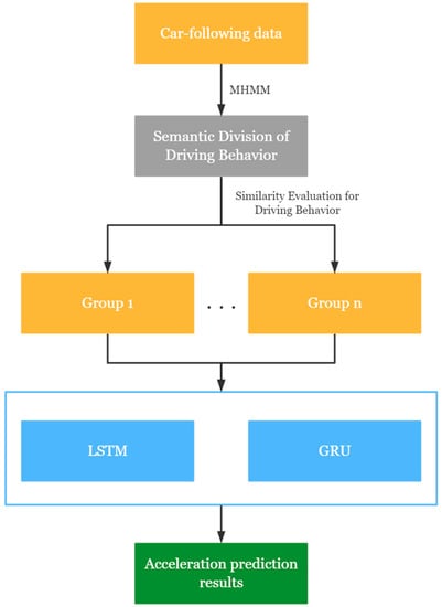
Figure 1.
Flowchart of the proposed vehicle acceleration prediction method.
2.1. HMM
The HMM includes two stochastic processes: the first one is the basic stochastic process that depicts the interconversion between states, i.e., a Markov chain; the second one is the stochastic process that depicts the correspondence between states and observations [13]. That is, the observer cannot observe the original state through the observations but can only use the stochastic process to determine the existence and characteristics of the model state.
In Figure 2, where is the hidden state, is the observation, is the transition probability of the hidden state, and is the output probability from the hidden state to the observed state. A complete definition of HMM is as follows:
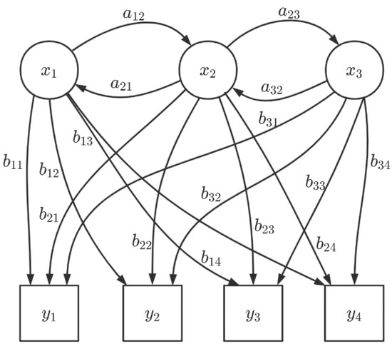
Figure 2.
A graphical model of the HMM.
and denote the set of all possible states, and the set of all possible observations, respectively.
where is the number of possible states and is the number of possible observation sequences.
is the state sequence of length , and is the observation sequence corresponding to :
A is the state-transferring probability matrix:
where is the probability of moving from moment in state to moment in state .
is the observation probability matrix:
where is the probability of obtain ing the observation under the condition of being in state at moment .
is the initial state probability vector:
where is the probability of being in state at moment .
The HMM is determined by the initial state probability vector , the state transferring probability matrix , and the observation probability matrix . and determine the state sequences, and determines the observation sequences. Thus, the HMM can be simplified as . In addition, as can be seen from the definition, the HMM makes two basic assumptions (i.e., the homogeneous Markov hypothesis and the observation independence assumption) [14].
2.2. MHMM
The car-following data used in this study are from the Safety Pilot Model Deployment (SPMD) database. The semantics of driving behavior may not be well divided by the traditional HMM, so we chose the MHMM, which can handle the heterogeneity of the data better. Meanwhile, when the model parameters are known, the probability of error in the partition estimation decreases exponentially with time [15]. The MHMM combines the HMM and the Finite Mixture Model (FMM). The HMM is a common type of Markov theoretical model that typically uses the observable parameters to calculate the unknown and hidden parameters in the model. Moreover, one advantage of the FMM over other clustering methods is that it can analyze hidden groups in the data [16]. The FMM clusters data with different features into different isomorphic sub-datasets to achieve data splitting by features. At the same time, each sub-dataset has its own feature parameters and distribution type, which is especially suitable for the large-sample continuous data in this study. In the FMM, assuming that the response variable comes with different categories , , , , the proportions are , , , , respectively. The density formula of the mixture model is [17]
where is the probability of category , and ; is the conditional probability density function of the response variable of the category . If is a member of the exponential families, as shown in Equation (6), the FMM can be combined with the HMM to obtain an MHMM. In this study, the maximum likelihood estimation method is used to estimate the parameters of the MHMM.
As shown in Figure 3, where is driver , is a car-following segment of driver , and is the driving behavior represented by the driving behavior semantics.
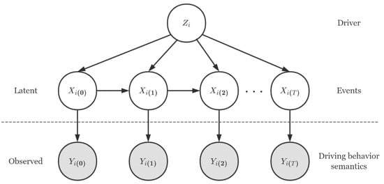
Figure 3.
A graphical model of the MHMM.
2.3. LSTM
In this study, after dividing driving behaviour semantics and similarity evaluation, acceleration is predicted in order to evaluate the effectiveness of the proposed personalized driving behaviour analysis method.
Because the driving state is a continuous time-lapse dependent process, the driver’s acceleration can be predicted using the complete time-series information. LSTM is a special type of Recurrent Neural Network (RNN) that can capture long-term temporal dependency. LSTM has a long-term memory function, which can deeply explore the long-term dependency and trend of limited data samples. Moreover, it can overcome the disadvantage of RNNs that they cannot perceive distance due to gradient disappearance during the training process [18].
LSTM has two transmission states between nodes, i.e., and . In the LSTM layer, the range of input information is controlled by input gates. The input from the previous node is selectively forgotten by forget gates. Finally, the recursion between the nodes is reached by outputting and through output gates. The mechanism of each stage is described as follows [19]:
Input gate:
Forget gate:
Status update:
Output gate:
where denotes the alternative values of the cell state at time ; denotes the output value of the hidden state at time ; denotes the input value of the memory cell at time ; and represent the cell state activation function and the gating activation function, respectively; and denotes the Hadamard product between the matrices.
2.4. GRU
GRU is a variant structure of LSTM. GRU combines the input and forget gates into update gates, and adds cell states and hidden states [20]. Compared with LSTM, GRU reduces the number of parameters required in the computation process by simplifying three gates into update and reset gates, which correspondingly shortens the time required for training and speeds up the convergence rate [21]. The brief structure of GRU is shown in Figure 4, and its computational equation is shown as follows:
where and are the states of the update gate and reset gate, respectively; is the output candidate set; and , and are the weights of the update gate, reset gate and output candidate set, respectively.
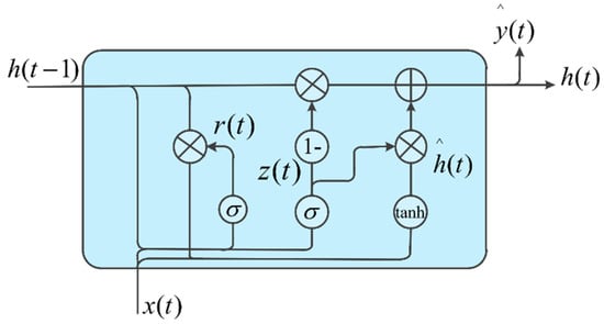
Figure 4.
The structure of the GRU network.
3. Personalized Driving Behavior Analysis Model
3.1. Data Description
All of the driving data we used were obtained from the SPMD database. This database recorded car-following data from 2842 equipment vehicles in the United States from 2012 to 2014. Overall, the SPMD data collection consisted of the surrounding environment (63 vehicles), light vehicle drivers (2836 drivers), heavy vehicle fleets (3 vehicles), and a transport vehicle fleet (3 vehicles). The light vehicle drivers were from the University of Michigan and its neighboring communities, and held valid driver’s licenses. The on-board devices include real-time data collection systems and Mobieye that continuously observe driving behavior over a period of time. The mobieye is responsible for recording road base information (e.g., the lane width, lane curvature, and number of lanes) and information about the surrounding vehicles (e.g., relative speed, relative distance). The information of the target vehicle is stored in a CAN-bus signal (e.g., speed, steering angle, pedal position). The data were collected at a frequency of 10 Hz. In addition, the driver cannot see the on-board devices while driving normally, which can avoid unnecessary interference to a certain extent [22].
We selected 30 drivers with similar driving scenes from the SPMD database and extracted their car-following trajectory data. This study did not consider data which were outliers, or missing frames greater than 1 s. For the missing durations of the follow-along fragment less than 1 s, this study used linear interpolation to make up for the missing duration [23]. In addition, we extracted the following conditions for car-following segments in the original data: (1) the lead vehicle and the subject vehicle are in the same lane; (2) the relative distance between two vehicles is less than 120 m and greater than 5 m; (3) the speed of the subject vehicle is greater than 18 km/h; (4) no overtaking event occurs; (5) the duration of a car-following segment is greater than 50 s [24].
A single variable, such as acceleration, does not characterize driving behavior well. Thus, environmental variables need to be included in order to help us analyze driving behavior. However, if we have too many variables, it will increase the calculation difficulty of the personalized driving behavior analysis model [25]. This study selects three characteristic variables from the SPMD, including the acceleration of subject vehicle , the relative distance and the relative speed between the subject vehicle and the lead vehicle [24].
This paper studied the driving behavior of drivers in a stable car-following scene. The driving environment is described by two variables, relative distance and relative speed, and the lead vehicles are all sedans. There are indeed some external environment variables that we did not consider, such as weather and traffic conditions, etc., because this information is not available in the SPMD dataset. These can be explored further when more complete car-following data information is available.
3.2. Semantic Division of the Driving Behavior
In order to better divide the semantics of the driving behavior, this study classifies the three characteristic variables into different classes according to the human velocity difference perception threshold, vestibular threshold, and kinesthetic threshold. The relative distances are classified into three classes [26], , and the relative speed and acceleration are each classified into five classes [27]: and . In the next section, the driving behavior semantics are utilized to evaluate the similarity between drivers. The classification criteria can be seen in Table 1.

Table 1.
Descriptions of the three feature variables.
According to the hidden state sequence of MHMM, this study obtains the trajectory segmentation results. Due to the space limitation, this study only shows the trajectory segmentation results for driver #1, as shown in Figure 5. The horizontal coordinates represent the time in seconds, and different color blocks represent different types of driving behavior semantics.
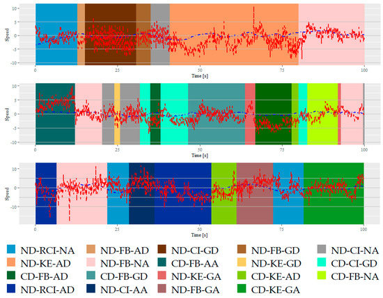
Figure 5.
Example of the segmentation results of three events for driver #1.
Figure 5 shows an example of the segmentation results using MHMM. As shown in Figure 5, MHMM can divide the driving speed sequence into various driving behavior segments. Effective behavior semantics are extracted based on the data distribution features. Besides this, the behavioral semantic segments are not very short (durations less than 1.0 s) because MHMM can better reduce the influence of random noise in the data compared with the traditional HMM [11]. The results show that MHMM can not only divide car-following data into multiple driving behavior semantics, but can also keep them within a reasonable duration.
Figure 5 indicates that when the distance from the lead vehicle is normal, the speed of the lead vehicle is less than that of the subject vehicle, and the subject vehicle rapidly closes in on the lead vehicle, then aggressively decelerates to fall behind from the lead vehicle, then slowly picks up speed to close in the lead vehicle and keeps a certain distance from it. At this time, the speed of the lead vehicle decreases, and the subject vehicle aggressively decelerates to fall behind from the lead vehicle. In this car-following segment, the driver kept a normal distance from the lead vehicle. The analysis process of the other two figures is similar to that of the first figure, which shows the driving behavior of the corresponding driver in this car-following segment.
Table 2 shows the statistical results of the durations of the driving behavior semantic. We found that the HMM obtained a larger number of driving behavior semantic segments than the MHMM. In addition, the MHMM obtained a lower percentage of semantic segments with durations less than 1.0 s than the HMM, which indicates that the MHMM can keep the semantic segments within a reasonable duration range better, and can match the actual driving habits.
Table 2.
Statistical results of the durations of the driving behavior semantic.
3.3. Similarity Evaluation for the Driving Behavior
Grouping drivers by similarity can facilitate the design of human-centric driver assistance systems. For example, drivers with similar driving behaviors can share the same driving behavior analysis model and driver assistance system [28]. However, human drivers are somewhat random and dynamic, and daily driving is highly nonlinear. Thus, the direct calculation of drivers’ observed statistical indicators (e.g., the mean and standard deviation) does not evaluate behaviors well [29]. In this study, a KS test was used for driving behavior similarity evaluation.
The Kolmogorov–Smirnov test (KS test) is a non-parametric test; it is based on the limiting distribution of the statistic as . For the hypothesis problem , The random variable has a distribution function of the form and is tested for significance. The steps are as follows [30]:
Step 1: The original hypothesis and alternative hypothesis are proposed, where is the empirical distribution function and is a certain distribution function of a known type.
Step 2: The sample size and the significance level are given.
Step 3: According to the limiting distribution of , there is , where , , is the upper quantile of the Kolmogorov distribution, which can be given by checking the Kolmogorov table.
Step 4: The rejection region of is given, i.e., if , is rejected; otherwise, is accepted.
In the above steps, the calculation of is cumbersome. Because the empirical distribution function is a step function, we have
In this study, the KS test is conducted using the driving behavior semantics, and then the similarity analysis is represented in heat maps. In Figure 6, crimson means a large difference in driving behavior and burgundy means a small difference in driving behavior. In addition to this, between the same drivers is represented in dark purple.
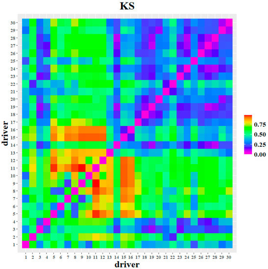
Figure 6.
KS test of the driving behaviour semantics between the drivers.
As shown in Figure 6, the KS test results for driver #11 were significantly different from other drivers such as drivers #5, #7, #8, #9, #15, and #16. In addition, driver #21 was similar to others such as the drivers #2, #3, #4, #6, #14, and #19. Last but not least, drivers #18, #19, #20, #23, #24, and #26–#30 were significantly similar to each other, as their color patches have similar colors and combinations.
By similarity evaluation, this study divided 10 similar drivers into group 1, and the other 20 drivers were classified as group 2. Based on the similarity evaluation results, this study built a vehicle acceleration prediction model in order to verify the effectiveness of the MHMM in dividing the semantics of driving behavior.
4. Discussion
4.1. Experimental Content
We used LSTM and GRU to predict vehicle acceleration in the car following condition. The experimental subjects are divided into three groups: 10 drivers with similar driving behaviors in group 1, and the other 20 drivers in group 2. In order to validate the performance of the proposed prediction approach, all 30 drivers were considered as the control group (group 3). In this study, the Min–Max function was used to normalize the data to improve the convergence speed and prediction performance of the model.
The LSTM model was implemented on a Windows platform based on a Tensorflow environment and optimized using Adaptive Momentum Estimation (Adam). All of the car-following data of each group were modeled separately, and 68% of the car-following segments were randomly selected as a training set, while the remaining 32% of the data were used as the test set. Each group was trained and predicted respectively, and therefore the model weights are different. Then, the number of neurons in the hidden layer and batch size were determined by the grid search method. Based on the experimental results, the super parameter values of the model are shown in Table 3.
Table 3.
Super parameter values of the LSTM model.
The GRU model was implemented on a Windows platform based on a Keras environment and optimized using Adam. The Adam optimization algorithm integrates the advantages of the AdaGrad and RMSProp algorithms for various gradient optimizations, and has the advantages of a simple operation and low memory requirements [31]. Therefore, both vehicle acceleration prediction models used the Adam algorithm as the first choice for the optimization of the error term. The data preprocessing of GRU was the same as LSTM, and then the grid search method was used to determine the super parameter values of the GRU, such as the number of hidden layers and the batch size. From the experiment, the super parameter values of the model are shown in Table 4.
Table 4.
Super parameter values of the GRU model.
In this study, we use mean the square error (MSE), root mean square error (RMSE) and mean absolute error (MAE) to evaluate the prediction accuracy of each model.
where is the true value and is the predicted value. MSE, RMSE and MAE all reflect the difference between the true and predicted values, and all three values fall into interval .
4.2. Experimental Results
The prediction performances of LSTM and GRU for three different driver subgroups are shown in Table 5. As shown in Table 5, the prediction accuracy of GRU is slightly better than LSTM in all three driver subgroups. This is because GRU can capture the nonlinear relationship of driver’s acceleration data and fits better than LSTM. The prediction of the subgroup of 10 drivers who have high similarity in driving behavior performs best. This is because the driving behaviors of these 10 drivers are semantically similar, and the computational difficulty and error of the model are greatly reduced compared to 30 drivers with different driving behaviors. In particular, for the comparison results of GRU, the MAE is reduced by 38.8%. As shown in Figure 7, the peak of the MSE and MAE of GRU appears earlier than that of LSTM, which also means that the GRU outperforms the LSTM [12]. Because the internal storage unit structure of GRU is simpler than LSTM, GRU is much faster than LSTM when training the model, and the prediction effect is slightly better than that of LSTM, and it is better than LSTM in processing car-following data [32]. In addition, the effectiveness of MHMM in the division of behavior semantics and the performance of similarity evaluation for building a better car-following prediction model was also verified.
Table 5.
Prediction performance of LSTM and GRU for different driver subgroups.
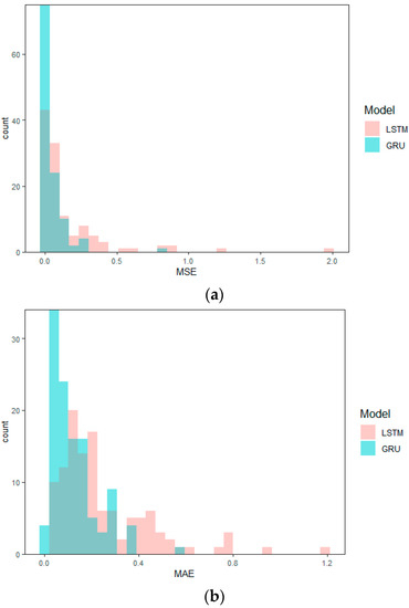
Figure 7.
Prediction results of 10 drivers. (a) Distribution of MSEs; (b) distribution of MAEs.
5. Conclusions
In this paper, we first proposed an MHMM personalized driving behavior analysis model for drivers in a car-following scene. The results of the semantic segmentation of the driving behaviors show that the MHMM can not only divide the car-following data into different behavioral semantic segments but also keep each segment within a reasonable duration. After that, similarity evaluation was performed based on the analysis results of the MHMM, and homogenous drivers were divided into a group. A controlled experiment was used to predict the drivers’ acceleration using both GRU and LSTM, and the experimental results verified the usefulness of the MHMM in personalized driving behavior analysis, and also showed that the performance of GRU is better than that of LSTM. For future work, the proposed car-following prediction approach can be applied to traffic data collected from other sites in order to further validate the findings from this study.
Author Contributions
Conceptualization, L.D. and H.Z.; methodology, L.D.; software, T.Z.; validation, Y.Z., L.D. and H.Z.; formal analysis, L.W.; investigation, Y.Z.; resources, Y.Z.; data curation, H.Z.; writing—original draft preparation, L.D. and H.Z.; writing—review and editing, Y.Z.; visualization, L.D.; supervision, Y.Z.; project administration, Y.Z.; funding acquisition, Y.Z. All authors have read and agreed to the published version of the manuscript.
Funding
This research received no external funding.
Institutional Review Board Statement
Not applicable.
Informed Consent Statement
Not applicable.
Data Availability Statement
All data and models used during the study appear in this article.
Acknowledgments
This research was funded by the National Natural Science Foundation of China (Grant No. 71971160) and the Fundamental Research Funds for the Central Universities (Grant no. 22120220013).
Conflicts of Interest
The authors declare no conflict of interest.
References
- Miyaji, M.; Danno, M.; Oguri, K. Analysis of driver behavior based on traffic incidents for driver monitor systems. In Proceedings of the Intelligent Vehicles Symposium, Eindhoven, The Netherlands, 4–6 June 2008; IEEE: Piscataway, NJ, USA, 2008. [Google Scholar]
- Aufrère, R.; Gowdy, J.; Mertz, C.; Thorpe, C.; Wang, C.C.; Yata, T. Perception for collision avoidance and autonomous driving. Mechatronics 2003, 13, 1149–1161. [Google Scholar] [CrossRef]
- Amin, M.S.; Reaz, M.; Nasir, S.S. Integrated Vehicle Accident Detection and Location System. TELKOMNIKA (Telecommun. Comput. Electron. Control.) 2014, 12, 73–78. [Google Scholar] [CrossRef][Green Version]
- Sato, T.; Akamatsu, M. Understanding driver car-following behavior using a fuzzy logic car-following model. In Fuzzy Logic—Algorithms, Techniques and Implementations; Book on Demand: Norderstedt, Germany, 2012; pp. 265–282. [Google Scholar]
- Wang, W.; Wei, Z.; Li, D.; Hirahara, K.; Ikeuchi, K. Improved action point model in traffic flow based on driver’s cognitive mechanism. In Proceedings of the Intelligent Vehicles Symposium, Parma, Italy, 14–17 June 2004. [Google Scholar]
- Agamennoni, G.; Nieto, J.I.; Nebot, E.M. A Bayesian approach for driving behavior inference. In Proceedings of the Intelligent Vehicles Symposium (IV), Baden-Baden, Germany, 5–9 June 2011; IEEE: Piscataway, NJ, USA, 2011. [Google Scholar]
- Wang, J.; Chen, R.; He, Z. Traffic speed prediction for urban transportation network: A path based deep learning approach. Transp. Res. Part C Emerg. Technol. 2019, 100, 372–385. [Google Scholar] [CrossRef]
- Jiang, B.; Fei, Y. Vehicle Speed Prediction by Two-Level Data Driven Models in Vehicular Networks. IEEE Trans. Intell. Transp. Syst. 2017, 18, 1793–1801. [Google Scholar] [CrossRef]
- Angkititrakul, P.; Miyajima, C.; Takeda, K. An improved driver-behavior model with combined individual and general driving characteristics. In Proceedings of the Intelligent Vehicles Symposium, Madrid, Spain, 3–7 June 2012. [Google Scholar]
- Harkous, H.; Bardawil, C.; Artail, H.; Daher, N. Application of Hidden Markov Model on Car Sensors for Detecting Drunk Drivers. In Proceedings of the 2018 IEEE International Multidisciplinary Conference on Engineering Technology (IMCET), Beirut, Lebanon, 14–16 November 2018. [Google Scholar]
- Vitali, W.; Ronja, F.; Yannis, P.; Iris, P.; Norman, W.; Jérémie, B. Using Hidden Markov Models to Improve Quantifying Physical Activity in Accelerometer Data—A Simulation Study. PLoS ONE 2014, 9, e114089. [Google Scholar]
- Fu, R.; Zhang, Z.; Li, L. Using LSTM and GRU neural network methods for traffic flow prediction. In Proceedings of the 2016 31st Youth Academic Annual Conference of Chinese Association of Automation (YAC), Wuhan, China, 11–13 November 2016; pp. 324–328. [Google Scholar]
- Schuster-Böckler, B.; Bateman, A. An introduction to Hidden Markov models. Curr. Protoc. Bioinform. 2007, 18, A–3A. [Google Scholar]
- Zhang, S.; Cao, C.; Quinn, A.; Vivekananda, U.; Litvak, V. Dynamic Analysis on Simultaneous iEEG-MEG Data via Hidden Markov Model. NeuroImage 2021, 233, 117923. [Google Scholar] [CrossRef]
- Chaumaray, M.; Marbac, M.; Navarro, F. Mixture of Hidden Markov models for accelerometer data. Ann. Appl. Stat. 2019, 14, 1834–1855. [Google Scholar]
- Baum, L.E.; Petrie, T. Statistical Inference for Probabilistic Functions of Finite State Markov Chains. Ann. Math. Stat. 1966, 37, 1554–1563. [Google Scholar] [CrossRef]
- Benaglia, T.; Chauveau, D.; Hunter, D.R.; Young, D.S. mixtools: An R Package for Analyzing Mixture Models. J. Stat. Softw. 2009, 32, 1–29. [Google Scholar] [CrossRef]
- Kong, W.; Dong, Z.Y.; Jia, Y.; Hill, D.J.; Xu, Y.; Zhang, Y. Short-term residential load forecasting based on LSTM recurrent neural network. IEEE Trans. Smart Grid 2017, 10, 841–851. [Google Scholar] [CrossRef]
- Hochreiter, S.; Schmidhuber, J. Long short-term memory. Neural Comput. 1997, 9, 1735–1780. [Google Scholar] [CrossRef] [PubMed]
- Peng, Z.; Peng, S.; Fu, L.; Lu, B.; Li, W. A novel deep learning ensemble model with data denoising for short-term wind speed forecasting. Energy Convers. Manag. 2020, 207, 112524. [Google Scholar] [CrossRef]
- Kisvari, A.; Lin, Z.; Liu, X. Wind power forecasting—A data-driven method along with gated recurrent neural network. Renew. Energy 2021, 163, 1895–1909. [Google Scholar] [CrossRef]
- Fitch, G.M.; Hanowski, R.J. Using Naturalistic Driving Research to Design, Test and Evaluate Driver Assistance Systems; Springer: London, UK, 2012. [Google Scholar]
- Bau, D. Numerical Linear Algebra: Numerical Linear Algebra; SIAM: Philadelphia, PA, USA, 1997. [Google Scholar]
- Wang, W.; Xi, J.; Zhao, D. Driving Style Analysis Using Primitive Driving Patterns With Bayesian Nonparametric Approaches. IEEE Trans. Intell. Transp. Syst. 2017, 20, 2986–2998. [Google Scholar] [CrossRef]
- Reesi, H.A.; Maniri, A.A.; Kai, P.; Hinai, M.A.; Adawi, S.A.; Davey, J.; Freeman, J. Risky driving behavior among university students and staff in the Sultanate of Oman. Accid. Anal. Prev. 2013, 58, 1–9. [Google Scholar] [CrossRef]
- Ahmed, K.I. Modeling Drivers’ Acceleration and Lane Changing Behavior. Ph.D. Thesis, Massachusetts Institute of Technology, Cambridge, MA, USA, 1999. [Google Scholar]
- Macadam, C.; Bareket, Z.; Fancher, P.; Ervin, R. Using Neural Networks to Identify Driving Style and Headway Control Behavior of Drivers. Veh. Syst. Dyn. 1998, 29, 143–160. [Google Scholar] [CrossRef]
- Wang, W.; Han, W.; Na, X.; Gong, J.; Xi, J. A Probabilistic Approach to Measuring Driving Behavior Similarity With Driving Primitives. IEEE Trans. Intell. Veh. 2019, 5, 127–138. [Google Scholar] [CrossRef]
- Nechyba, M.; Xu, Y. Stochastic Similarity For Validating Human Control Strategy Models. IEEE Trans. Robot. Autom. 1998, 14, 437–451. [Google Scholar] [CrossRef]
- Hollander, M.; Wolfe, D.A.; Chicken, E. Nonparametric Statistical Methods; John Wiley & Sons, Inc.: Hoboken, NJ, USA, 2008. [Google Scholar]
- Jais, I.K.M.; Ismail, A.R.; Nisa, S.Q. Adam optimization algorithm for wide and deep neural network. Knowl. Eng. Data Sci. 2019, 2, 41–46. [Google Scholar] [CrossRef]
- Wang, C.; Du, W.B.; Zhu, Z.X.; Yue, Z.F. The real-time big data processing method based on LSTM or GRU for the smart job shop production process. J. Algorithms Comput. Technol. 2020, 14, 1748302620962390. [Google Scholar] [CrossRef]


Publisher’s Note: MDPI stays neutral with regard to jurisdictional claims in published maps and institutional affiliations. |
© 2022 by the authors. Licensee MDPI, Basel, Switzerland. This article is an open access article distributed under the terms and conditions of the Creative Commons Attribution (CC BY) license (https://creativecommons.org/licenses/by/4.0/).