Featured Application
Deep-level transient spectroscopy; any applications requiring extraction of rate and initial value of decaying exponentials.
Abstract
A mathematical method is presented for the extraction of defect parameters from the multiexponential decays generated during deep-level transient spectroscopy experiments. Such transient phenomenon results from the ionization of charge trapped in defects located in the depletion width of a semiconductor diode. From digitized transients acquired at fixed temperatures, this method produces a rate–domain spectral signature associated with all defects in the semiconductor. For signal-to-noise ratio of 1000, defect levels with carrier emission rates differing by as little as 1.5 times may be distinguished.
1. Introduction
Exponential transients are common in nature. The decay rates and initial values of these transients offer valuable insight into the underlying physics of their source. In semiconducting systems, both optical and electrical transients are used to characterize both bulk material and discrete devices. Deep-level transient spectroscopy (DLTS) is an experimental technique which analyzes exponentially decaying capacitance transients resulting from the emission of trapped charges from defects found in the depletion region of a diode [1]. Methods used to extract pertinent results from these transients are the basis of this and other works [1,2,3,4,5,6,7].
Semiconductor-based components in harsh environments, such as infrared sensors in space, accumulate electrically active defects due to radiation damage [8,9,10,11,12,13,14]. Such defects act as recombination and charge compensation centers and thereby affect minority carrier lifetime and free carrier concentration, which degrade circuit functionality. The ability to observe and understand the formation, evolution, and mitigation of defects in semiconductors is essential to prolonging the useful life of electronics and optoelectronics in harsh environments [15,16,17]. Accuracy and the ability to resolve closely spaced energy levels are important for a fundamental understanding of these defects. This paper presents an improved technique for analyzing capacitance transients at constant stable temperatures. The technique allows defect-level determination with higher accuracy and resolution than current approaches.
2. Methods
To investigate defects in semiconducting systems, the ionization or emission rate of trapped carriers R(T) is typically used, and is given by
where is temperature and is Boltzmann’s constant. The ionization energy, , and the capture parameter, , are unique defect-specific signatures, both required for an a priori determination of emission rate at a specific temperature. If the capture parameter and ionization energy are not known a priori, then the emission rate must be determined as a function of temperature. Once obtained, the capture parameter and ionization energy are extracted using Arrhenius analysis of R(T) [1,18].
In practice, a capacitance transient is obtained by collapsing a diode’s depletion region for a time, , filling the defect sites with carriers [19]. A reverse bias is then applied at t = 0 to expand the depletion region and initiate defect ionization at rates determined by the ionization energy and capture parameter in Equation (1). Changes to diode capacitance occur as the diode depletion width expands or contracts to maintain charge neutrality in the depletion region of the diode as defect ionization occurs. This fill-and-measure sequence produces a capacitance transient, as shown in Figure 1, with the initial value ±C, with respect to a steady state value B. The capacitance transient is of the form
where is proportional to the defect concentration, with a positive sign consistent with minority carrier emission and a negative sign indicating majority carrier emission. The sign of C is the strength of the capacitance-based DLTS technique. Similar current–transient-based techniques cannot distinguish between minority carrier or majority carrier emissions, because each carrier contributes identically to any current measured [20,21,22].
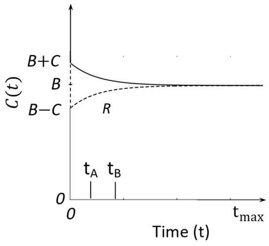
Figure 1.
DLTS capacitance transients for minority carriers (solid line) and majority carriers (dashed line), following the removal of a fill pulse at time t = 0. tA and tB represent sampling times for a waveform sampled for a total time, tmax.
The constant value B is not a function of time, only of temperature, and represents the case of complete defect ionization. In practice, the temperature dependence of the background signal, B(T), complicates transient analysis because, a priori, it is not known whether the background is a constant or a very slowly ionizing defect site. The SLAP methodology presented below effectively removes this ambiguity.
Traditionally, the capacitance transients of DLTS were repeated and averaged using an analog boxcar average [1]. The double-boxcar average technique was configured to sample a repeated input signal at two chosen times, and , which define a rate window. This analog gated measurement was synchronized with the start of defect ionization, producing a derived signal, as follows:
Then, for traditional capacitance-based DLTS, temperature is slowly swept, and a peak in the DLTS signal is found at some temperature, Tpeak, when the emission rate is given by
The double-boxcar average output is then plotted versus temperature to produce a set of Tpeak,i, each of which defines an emission rate, Ri, for the ith defect, according to Equation (4). Each Tpeak,i contributes to the spectral signature unique to the type (donor or acceptor), concentration, capture parameter, and ionization energy of all defects present. Analysis of a DLTS signal deconvolves this signature into an integer number of specific defects. Because traditional capacitance-based DLTS requires a temperature scan to determine the temperature which maximizes the DLTS signal, each data point requires the system to first come into temperature equilibrium with its surroundings, followed by any signal averaging required to improve the signal-to-noise ratio. This effort produces a single point of the traditional DLTS, the temperature domain spectrum. The SLAP methodology also requires the temperature to equilibrate followed by signal averaging to improve the signal-to-noise ratio. However, the SLAP transform algorithm effectively searches for that rate window which will maximize the SLAP signal at the current temperature, with minimal computational overhead. Thus, the SLAP methodology can produce a full rate domain spectrum in the time it takes to produce one point of a DLTS temperature domain spectrum.
Although relatively simple for a single defect, the challenge is to resolve the signatures of multiple defects, whose concentration, type, and ionization parameters are unknown [2,3,4,5,6,7,23,24,25,26]. In traditional boxcar-based, temperature-swept DLTS, two neighboring peaks can be distinguished if their emission rates differ by at least ~8 times [6]. Other, more recent DLTS analysis techniques utilize the Laplace transform (L-DLTS) or Fourier transform (deep-level Fourier spectroscopy) to improve signal acquisition and rate extraction to improve emitter distinguishability [6,7,23]. Both techniques are constant-temperature approaches, such as the SLAP technique, allowing for unlimited signal averaging for improved signal-to-noise ratio. Both techniques offer improvements over the original double-boxcar technique in that the judgment of the user is not required to determine peak location in temperature or rate, instead relying on curve-fitting algorithms to obtain peak location and height, sharing a similar strength with the proposed SLAP technique. Both L-DLTS and deep-level Fourier spectroscopy identify defects as a spectral feature, as does SLAP, with the SLAP technique offering minimal computational overhead and a simple curve-fitting function for peak characterization. Significantly, both L-DLTS and Fourier spectroscopy are based on integrals summed from zero to infinity. This is in stark contrast to the SLAP technique, which obtains results as an integer sum with each integer representing a unique defect. As will be shown, the SLAP technique also provides both minority and majority carrier defect information from a single transient. In all cases, a constant-temperature approach is used for more precise determination of defect parameters through signal averaging, with a signal-to-noise ratio of at least 1000 required for Laplace DLTS to provide better rate resolution than offered by the traditional double-boxcar DLTS technique [23].
3. Results
We present a mathematical “sliding-aperture” transform (or SLAP) to obtain defect parameters from capacitance transients measured at constant temperature. Each capacitance transient is an integer sum over defect species of exponential transients, Equation (2), each with its own set of parameters, Ci, and Ri, where the subscript “i” enumerates the defects. For any fixed temperature, there is a single constant offset, B, corresponding to the quiescent reverse bias capacitance value at infinite time when all defects have been ionized. The SLAP transform is plotted as a function of the rate variable ρ = 1/t and produces a defect signature composed of a set of peaks whose locations identify the rates Ri, and whose peak values define the peak capacitances Ci. Spectra taken at different fixed temperature will have defect signatures shifted to different positions on the ρ axis, according to Equation (1). Analysis of the temperature dependence of the obtained values then gives the desired defect parameters and . Like traditional DLTS, the background, B, subtracts out and needs to be determined by other means to accurately determine defect concentration from the transient maximum.
The SLAP transform is defined as
where all quantities are evaluated at the same constant temperature and the SLAP function is expressed in terms of the rate variable ρ = 1/t. The aperture N is defined as
where tA represents the first sampled time after the removal of the fill pulse. In the simplest case, for a transient sampled at a fixed sampling period, the first few ordered pairs of the SLAP transform for the N = 2 case will be:
Any waveform, sampled at a fixed sampling rate, can be SLAP-transformed using the above algorithm. This work concentrates on the special case, where the original function is of the form of Equation (2), namely a decaying exponential plus a constant baseline. This leads to the following SLAP function:
Transforming a digital waveform, as described above, will lead to a waveform that can be curve-fit with the SLAP function of Equation (7). Alternatively, the SLAP function of Equation (7) can be used as an equivalent representation of the decaying exponentials of Figure 1 with the constant background, B(T), eliminated, as shown in Figure 2. Here, a positive and a negative SLAP peak are plotted in the inverse time, or rate domain , on axis, with the axis scaled by factors notated as and . These scale factors are obtained by first noting that the SLAP peak will be located at R, where,
with direct substitution of Equation (8) into (7) leading to
which defines both the and scaling factors.
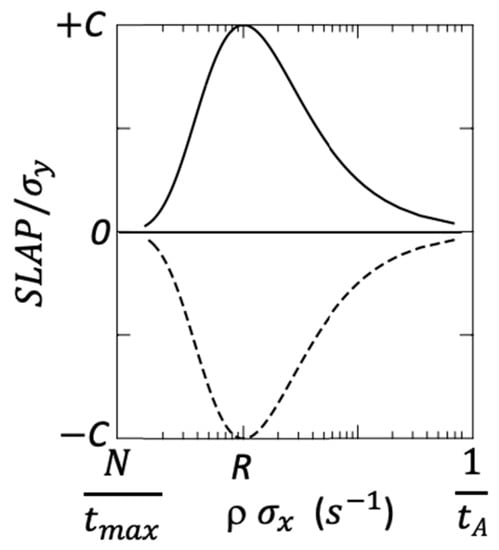
Figure 2.
SLAP transformation of the decaying exponentials of Figure 1.
In general, each defect species is characterized by the physical attributes associated with Equation (1), namely emission rate and capture parameter. This leads to the SLAP transformation for multiple emitters as an integer sum of the following form:
which produces k peaks, each of which defines a pair of defect parameters (Ri, Ci).
The strength of the SLAP approach to transient analysis is the ability to use Equation (10) and a simple curve-fitting algorithm to curve-fit a multipeak spectrum based on an integer number of defects. This removes user intervention from the process of rate and peak height determination and is not only the strength of this work but is prominent attribute for both L-DLTS and deep-level Fourier spectroscopy [6,7,23]. SLAP offers another means of characterizing defect spectrum through the sequential use of Equation (10), first under the assumption of a single defect (i.e., i = 1, k = 1), followed by the introduction of more defect species (i.e., k > 1).
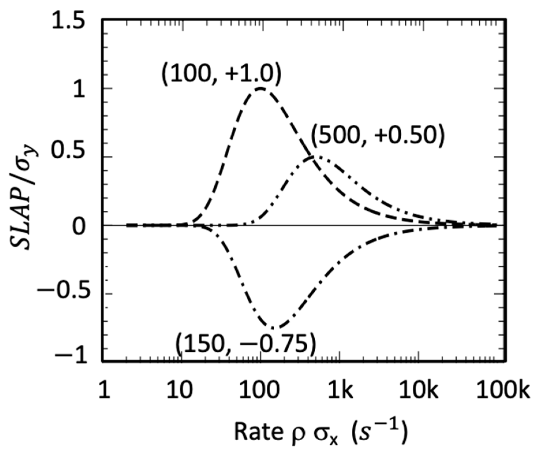
This algorithm is now used to assess the effect of noise on rate and maximum value extraction from simulated noise-loaded transients using Equation (10). The simultaneous ionization of two majority and one minority defect species, the SLAP transforms of which are shown individually in Figure 3, were summed and simulated with noise added. Signal-to-noise ratios, S/N, of 20, 50, and 1000 were investigated, with the superposition in the worst-case S/N = 20 plotted in Figure 4. Curve-fitting was proceeded by assuming one–four defects with unconstrained signs for the Ci. For all simulations a sampling period of 0.2 s−1 was used with 105 sampled points. Convergence was obtained in cases of one–three defects with results shown. No convergence or vanishingly small Ci values were obtained in the four-defect case. The three-defect case gave the best fit for all S/N considered. When S/N = 1000, the obtained defect parameters (Ri, Ci) were the same as indicated in Figure 2 within 1%. When S/N = 20, obtained values of (91, +0.7), (176, −0.46), and (496, 0.51). These values differ from the input values by (9, 30), (17, 39), and (1, 2)%, respectively. The simulations suggest that SLAP peaks can be resolved when S/N = 1000 if their rates differ by as little as a factor of 1.5.
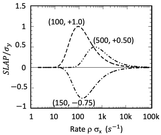
Figure 3.
SLAP transforms of two majority and one minority carrier defects with decay rates and maximum values shown as ordered pairs.
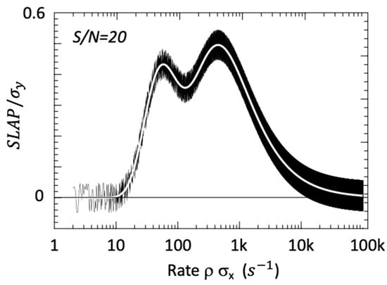
Figure 4.
Superposition of SLAP peaks with added noise (S/N = 20) and best fit assuming three defects.
4. Discussion
We introduced the SLAP transform as a means to deconvolve the multiexponential capacitance transients often observed during DLTS investigations of defects in semiconducting materials. Its application to the analysis of noise-laden capacitance transients at constant temperature was used to illustrate the strength of the derived SLAP function as an aid in the determination of the type, decay rate, maximum value, and number of each emitter present. This work suggests the SLAP transform should provide exceptionally high resolving power to distinguish defects with ionization rates different by as little as 1.5 for signal-to-noise ratios of 1000.
SLAP may be applied to determine rate constants for other types of decays. For instance, it has recently been used in the analysis of laser propagation decay in scattering media [27]. This work neatly demonstrates the value of SLAP to determine decay constants when there is an unknown background.
Author Contributions
Conceptualization, W.R.B.; methodology, W.R.B.; software, W.R.B.; validation, R.E.P., C.P.M., P.C.G., J.V.L. and P.T.W.; writing—original draft preparation, W.R.B.; writing—review and editing, R.E.P., C.P.M., P.C.G., J.V.L. and P.T.W. All authors have read and agreed to the published version of the manuscript.
Funding
This research received no external funding.
Institutional Review Board Statement
Not applicable.
Data Availability Statement
Not applicable.
Acknowledgments
W.R.B. acknowledges the Air Force Office of Scientific Research, Gernot Pomrenke, and the Air Force Summer Faculty Fellowship Program for support of the ideas presented in this work.
Conflicts of Interest
The authors declare no conflict of interest.
References
- Lang, D. Deep-level transient spectroscopy: A new method to characterize traps in semiconductors. J. Appl. Phys. 1974, 45, 3023. [Google Scholar] [CrossRef]
- Hanak, T.R.; Ahrenkiel, R.K.; Dunlavy, D.J.; Bakry, A.M.; Timmons, M.L. A new method to analyze multiexponential transients for deep-level transient spectroscopy. J. Appl. Phys. 1989, 67, 4126. [Google Scholar] [CrossRef]
- Ikossi-Anastasiou, K. Refinements in the method of moments for analysis of multiexponential capacitance transients in deep-level transient spectroscopy. J. Appl. Phys. 1987, 61, 182. [Google Scholar] [CrossRef]
- Ransom, C.M.; Chappell, T.I.; Freeouf, J.L.; Kirchner, P.D. Modulating functions waveform analysis of multiexponential transients for deep-level transient spectroscopy. Mater. Res. Soc. Symp. Proc. 1986, 69, 337. [Google Scholar] [CrossRef]
- Kirchner, P.D.; Schaff, W.J.; Maracas, G.N.; Eastman, L.F.; Chappell, T.I.; Ransom, C.M. The analysis of exponential and nonexponential transients in deep-level transient spectroscopy. J. Appl. Phys. 1981, 52, 6462. [Google Scholar] [CrossRef]
- Dobaczewski, L.; Peaker, A.R.; Nielsen, K.B. Laplace-transform deep-level spectroscopy: The technique and its applications to the study of point defects in semiconductors. J. Appl. Phys. 2004, 96, 4689. [Google Scholar] [CrossRef] [Green Version]
- Ikeda, K.; Takaoka, H. Deep level Fourier Spectroscopy for Determination of Deep Level Parameters. Jpn. J. Appl. Phys. 1982, 21, 462. [Google Scholar] [CrossRef]
- Farzana, E.; Chaiken, M.F.; Blue, T.E.; Arehart, A.R.; Ringel, S.A. Impact of deep level defects induced by high energy neutron radiation in β-Ga2O3. APL Mater. 2019, 7, 022502. [Google Scholar] [CrossRef] [Green Version]
- Kim, J.; Pearton, S.; Fares, C.; Yang, J.; Ren, F.; Kim, S.; Polyakov, A. Radiation Damage Effects in Ga2O3 Materials and Devices. J. Mater. Chem. C 2019, 7, 10. [Google Scholar] [CrossRef]
- Kumar, A.; Dhillon, J.; Verma, S.; Kumar, P.; Asokan, K.; Kanjilal, D. Identification of swift heavy ion induced defects in Pt/n-GaN Schottky diodes by in-situ deep level transient spectroscopy. Semicond. Sci. Technol. 2018, 33, 085008. [Google Scholar] [CrossRef]
- Li, Z. Radiation damage effects in Si materials and detectors and rad-hard Si detectors for SLHC. JINST 2009, 4, P03011. [Google Scholar] [CrossRef]
- Summers, G.P.; Burke, E.A.; Walters, R.J. Damage correlations in semiconductors exposed to gamma, electron and proton radiation. IEEE Trans. Nucl. Sci. 1993, 40, 1372–1379. [Google Scholar] [CrossRef] [Green Version]
- Morath, C.P.; Cowan, V.M.; Treider, L.A.; Jenkins, G.D.; Hubbs, J.E. Proton Irradiation Effects on the Performance ofIII-V-Based, Unipolar Barrier Infrared Detectors. IEEE Trans. Nucl. Sci. 2015, 62, 512–519. [Google Scholar] [CrossRef]
- Lee, J.; Kim, H.; Jeong, H.; Cho, S. Optimization of shielding to reduce cosmic radiation damage to packaged semiconductors during air transport using Monte Carlo simulation. Nucl. Eng. Technol. 2020, 52, 1817. [Google Scholar] [CrossRef]
- Oda, T.; Arai, T.; Furukawa, T.; Shiraishi, M.; Sasajima, Y. Electric-Field-Dependence Mechanism for Cosmic Ray Failure in Power Semiconductor Devices. IEEE Trans. Electron Dev. 2021, 68, 3505–3512. [Google Scholar] [CrossRef]
- Wesch, W.; Wendler, E.; Schnohr, C.S. Damage evolution and amorphization in semiconductors under ion irradiation. Nucl. Inst. Meth. Phys. Res. B 2012, 277, 58. [Google Scholar] [CrossRef]
- Zeller, H. Cosmic ray induced failures in high power semiconductor devices. Solid State Electron. 1995, 38, 2041. [Google Scholar] [CrossRef]
- Wickramaratne, D.; Dreyer, C.E.; Monserrat, B.; Shen, J.-X.; Lyons, J.L.; Alkauskas, A.; van de Walle, C.G. Defect identification based on first-principles calculations for deep level transient spectroscopy. Appl. Phys. Lett. 2018, 113, 192106. [Google Scholar] [CrossRef] [Green Version]
- Criado, J.; Gomez, A.; Calleja, E.; Munoz, E. Novel method to determine capture cross-section activation energies by deep-level transient spectroscopy techniques. Appl. Phys. Lett. 1988, 52, 660. [Google Scholar] [CrossRef]
- Balland, J.C.; Zielinger, J.P.; Noguet, C.; Tapiero, M. Investigation of deep levels in high-resistivity bulk materials by photo-induced current transient spectroscopy. I. Review and analysis of some basic problems. J. Phys. D Appl. Phys. 1986, 19, 57. [Google Scholar] [CrossRef]
- Blood, P.; Orton, J.W. The electrical characterization of semiconductors. Rep. Prog. Phys. 1978, 41, 157. [Google Scholar] [CrossRef]
- Cui, Y.; Bhattacharya, P.; Burger, A.; Johnstone, D. Photo-induced current transient spectroscopy and photoluminescence studies of defects in AgGa0.6In0.4Se2. J. Phys. D Appl. Phys. 2013, 46, 305103. [Google Scholar] [CrossRef]
- Emiroglu, D.; Evans-Freeman, J.; Kappers, M.J.; McAleese, C.; Humphreys, C.J. High Resolution Laplace Deep Level Transient Spectroscopy Studies of Shallow and Deep Levels in n-GaN. In Proceedings of the IEEE 2008 Conference on Optoelectronic and Microelectronic Materials and Devices, Sydney, NSW, Australia, 28 July–1 August 2008. [Google Scholar]
- Buchwald, W.R.; Morath, C.P.; Drevinsky, P.J. Effects of deep defect concentration on junction space charge capacitance measurements. J. Appl. Phys. 2007, 101, 094503. [Google Scholar] [CrossRef]
- Buchwald, W.R.; Johnson, N.M.; Trombetta, L.P. New metastable defects in GaAs. Appl. Phys. Lett. 1987, 50, 1007. [Google Scholar] [CrossRef]
- Arora, B.M.; Chakravarty, S.; Subramanian, S.; Polyakov, V.I.; Ermakov, M.G.; Ermakova, O.N.; Perov, P.I. Deep-level transient charge spectroscopy of Sn donors in AlxGa1−xAs. J. Appl. Phys. 1991, 73, 1802. [Google Scholar] [CrossRef]
- Peale, R.E.; Fredricksen, C.J.; Barrett, C.L.; Otero, A.G.; Jack, A.R.; Gonzalez, F.J.; Sapkota, D.; Dove, A.R.; Metzger, P.T. Laser Particle Sizer for Plume-Induced Ejecta Clouds. In Laser Radar Technology and Applications XXVII, Proceedings of the PIE Conference on Defense + Commercial Sensing, Orlando, FL, USA, 3–8 April 2022; Kamerman, G.W., Magruder, L.A., Turner, M.D., Eds.; SPIE: Bellingham, WA, USA, 2022; Volume 12110, Paper # 2. [Google Scholar]


Publisher’s Note: MDPI stays neutral with regard to jurisdictional claims in published maps and institutional affiliations. |
© 2022 by the authors. Licensee MDPI, Basel, Switzerland. This article is an open access article distributed under the terms and conditions of the Creative Commons Attribution (CC BY) license (https://creativecommons.org/licenses/by/4.0/).