Communication

Mathematical Modeling and Optimal Control for a Class of Dynamic Supply Chain: A Systems Theory Approach

by
Heidi Taboada
1,
Yasser A. Davizón
2,*,
José F. Espíritu
1 and
Jaime Sánchez-Leal
3
1
Mechanical and Industrial Engineering, Texas A&M University-Kingsville, 700 University Blvd, Kingsville, TX 78363, USA
2
Department of Information Technology, Universidad Politécnica del Mar y la Sierra, Potrerillos del Norote, Tayoltita 82740, Mexico
3
Industrial, Manufacturing and Systems Engineering, The University of Texas at El Paso, 500 West University Avenue, El Paso, TX 79968, USA
*
Author to whom correspondence should be addressed.
Appl. Sci. 2022, 12(11), 5347; https://doi.org/10.3390/app12115347
Submission received: 14 April 2022 / Revised: 19 May 2022 / Accepted: 23 May 2022 / Published: 25 May 2022

Abstract

:

Featured Application

Dynamic supply chains are suitable for the mathematical modeling, analysis and control of high-volume manufacturing supply chains in which low variability is present, considering a cause–effect relation in a deterministic context. The application of ordinary differential equations via the mixing problem context is addressed.

Abstract

Dynamic supply chains (SC) are important to reduce inventory, enable the flow of materials, maximize profits, and minimize costs. This research work presents a capacity–inventory management model via system dynamics for a dynamic supply SC, applying model-based optimal control techniques. In the context of high-volume manufacturing (HVM) that present low variability and predictable demand, for mathematical modeling purposes, a set of coupled first-order ordinary differential equations, with an analogy from the mixing problem, is presented, which relates capacity and inventory levels, taking into account a production rate at each node of interaction. The application of ordinary differential equations via the mixing problem (or compartmental analysis) is important based on the idea of a balance between the influx and outflux of raw material along the supply chain. A proper literature review on optimal control for supply chains is analyzed. The mathematical model introduced is presented in a linear time-invariant (LTI) state-space formulation. Stability analysis for the dynamic serial SC is presented, and a sensitivity analysis is also conducted for the capacity and production rate parameters considering the effects of variations in parameters along the SC. An energy-based optimal control is also developed with proper simulations.

1. Introduction

Dynamic supply chains present novel approaches from mathematical modeling, control and stability analysis approaches. In the context of mathematical modeling, the use of ordinary differential equations (ODE), difference equations and partial differential equations (PDE) are suitable for model-based, control-oriented approaches.
Several applications have been reported in dynamic supply chains: in [1], they applied optimal control to dynamic food supply chains; in [2], they created a dynamic optimization model by applying a real option on stochastic demands; and in [3], a fuzzy hybrid negotiation mechanism for dynamic SC is present, as well as in [4]. The purpose of this article is to consolidate the existing issues related to information systems in dynamic SC.
In this research work, our aim is to focus on model-based optimal control theory. In terms of stability analysis, our goal is to analyze the stability of the dynamic SC by the application of linear and nonlinear systems.
In operations and production-planning processes, decision-makers develop convenient and suitable decisions to validate their hypothesis about which decisions incorporate more profit while reducing costs on enterprise operations. In this way, a dynamic SC requires proper decision-making with effective performance and synchronization. In general, an SC processes raw material, cash, and information flows, taking into account the demand profile of the system. Manufacturing converts raw materials into end products within a demand profile. However, these manufacturing systems face problems, such as: long downtime, labor inefficiency, inaccurate scheduling, and weak energy consumption [5]. Recently, supply chain (SC) market forecasts in profitability have been increasing. Based on this, nowadays, SC has gained special attention among industry practitioners of automation science and control systems. SC applications in industry can integrate potential solutions, such as automotive, aerospace, biotechnology, energy, etc. Considering that manufacturing systems are dynamic and complex [6], the proper design of control systems requires flexibility and should be adaptive to process disturbances. In this context, new trends are required to take into account systems theory and control theory perspectives in order to support accurate, agile, and flexible solutions for SC applications. Industrial production systems require competitive and adaptive solutions in order to ensure profitability in markets. In manufacturing systems, decision-makers are required to achieve and approximate online decisions. A manufacturing SC is a system composed of suppliers, manufacturers, distributors, and customers that serves customer requirements [7]. SC integrates solutions to decrease operation management costs such as production, logistics, and quality. In this context, dynamic approaches for production–inventory systems are valuable in order to maximize profits and minimize costs throughout the SC system. Recently in SC, the focus has moved from the factory-level management to a more enterprise-level [8].
Inventory management presents a crucial role through the performance analysis of a supply chain. By definition, inventory management is “the continuing process of planning, organizing, and controlling inventory while balancing supply and demand” [9]. In this research work, our main interest is to provide modeling, analysis, and model-based optimal control for a dynamic SC from a systems theory perspective. Designing an inventory management system is directly related to sales, finance, production, and procurement [10]. Moreover, the goal of inventory management is to minimize the average cost per unit of time experienced for the inventory system in the long run [11]. Considering that decision variables are related to inventory levels along the SC, and production rate and capacity levels are fixed parameters, this paper presents the mixing problem as an analogy for an approximation of a four-echelon supply chain. Ordinary differential equation application for mathematical modeling purposes via the mixing problem is important in high-volume manufacturing supply chains.
In the context of dynamic SC, inventory management (IM) presents an important role in the operation and management sciences. In this research work, our aim is to present a systemic analysis regarding the reasons why IM for dynamic SC is important by applying systems theory and model-based control approaches. The main goal is to explore the dynamic nature of SC via the development of ordinary differential equations (linear and nonlinear). By definition, inventory management is part of the SCM, which plans, implements, and controls the forward and reverse flow of goods and services (as well as storage) between the point of origin and the point of consumption to meet customer requirements. Inventories, by their nature, are present all along the supply chain (SC), and inventory control is a crucial activity by a company’s management [12].
Presenting appropriate inventory levels is a crucial task for a company [13], considering that quick and positive response to customers is related to high inventory levels (which increase the cost), while low inventory levels might cause scarcity. In general, for manufacturing firms, inventory usually represents from 20% to 60% of the total assets [14]. The coordination of inventory policies in IM for SCM between suppliers, manufactures, and distributors is a major task. Furthermore, it smooths material flow and minimizes costs while meeting customer demands [15].
Based on this, the following research questions are formulated: (1) Are dynamic supply chains suitable to be mathematically modeled via the mixing problem? (2) Do optimal control and high-volume manufacturing have an impact at operational level of dynamic SC?
The rest of the paper is organized as follows: Section 2 presents an analysis on dynamic SC and the role of optimal control theory in supply chains. Section 3 presents a discussion of the mixing problem theory. A mathematical modeling description of the problem, as well as a sensitivity and stability analysis for the system, are present in Section 4. In Section 5, a model-based optimal control for a composed energy performance index is presented. In Section 6, a discussion on the results is presented. Finally, conclusions and future work are discussed in Section 7.

2. Dynamic Supply Chains

By definition, SCM integrates suppliers, manufacturers, warehouses, and stores in order to minimize costs and satisfy service requirements. In SCM, the decision-making process consists of strategical, tactical, and operational levels. In this section, we explore the impact of high-volume manufacturing in SCM and the optimal control for supply chains.

2.1. High-Volume Manufacturing

The main consideration for inventory management policies along the SCM are: (Ryu, et al, 2013) (1) type of optimization; (2) control system type (centralized or distributed); (3) inventory levels nature; (4) demand function type (stochastic or deterministic), and (5) inventory control responsibility. In high-volume manufacturing (HVM), the determinant of inventory levels assesses the amount of raw materials, work in progress, and finished goods inventories along the SCM [16].
In general, HVM is used to fabricate large quantities of goods in short periods of time. Products that are produced in high volume present low variability. HVM permits manufacturers to produce goods in a fast manner. In HVM, the demand is predictable, which implies that companies can produce with anticipation, avoiding the possibility of carrying excess or obsolete inventory. Posssible manufacturing strategies in HVM are: assembly lines, make to stock, and factory-level loading.
Therefore, HVM conventionally involves the introduction of automation and control system techniques for manufacturing and assembly processes. Our aim in this research work is to present the use of optimal control theory as a control system strategy based on the context that a mathematical model should be present. In order to conduct the application of the Pontryagin maximum principle, the description of our system dynamics via ordinary differential equations is mandatory. In general, for dynamic SC, enterprises should design and select their business models and inventory levels based on real demand compared to forecasted demand.
The application of optimal control and mathematical modeling, in our context, assumes deterministic modeling and a cause-effect relation in which the demand and inventory levels are related; refer to Figure 1.

2.2. Optimal Control Theory in Supply Chains

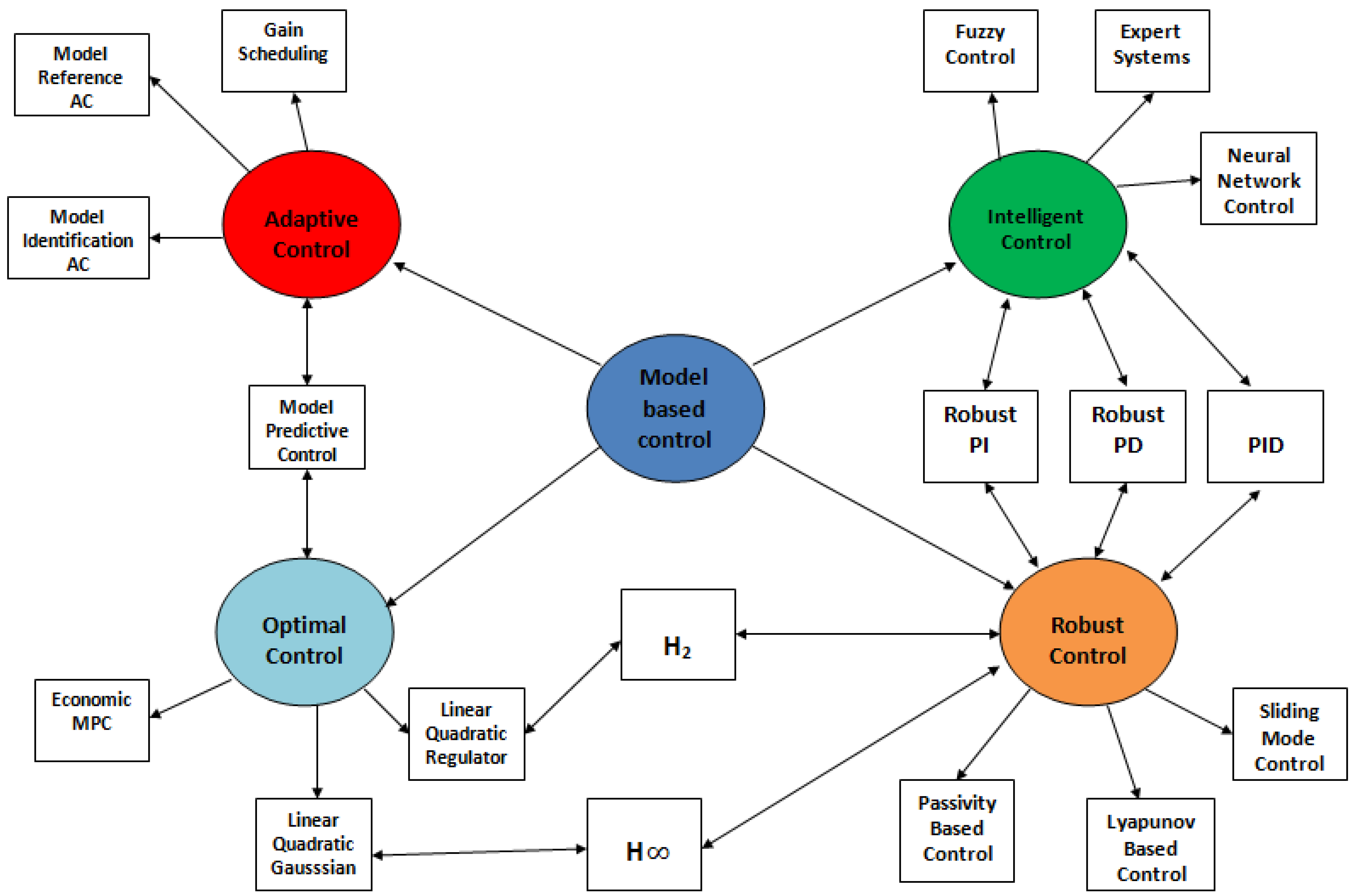
Control theory relates the core idea of maintaining equilibrium and a stability state through uncertainty and disturbance [17]. The modeling and analysis of control systems present the following taxonomy: model-based control and data-driven control. In general, model-based control has the following subclassifications: optimal control, robust control, adaptive control, and intelligent control.
In Figure 2, a general taxonomy is presented for model-based control systems, which incorporates: optimal control, robust control, intelligent control and adaptive control. The most common model-based control system strategies nowadays are control structures, which have, in general, been applied in oil, aerospace, automotive, and manufacturing industries.
Supply chains present a dynamical behavior where, from a model-based optimal control perspective, the following approaches are present: (1) classical control theory, (2) optimal control theory, and (3) model predictive control. Our aim in this research work is to develop optimal controls, which have been analyzed via the Pontryagin maximum principle in the context of dynamic supply chains.
In general, optimal control theory requires a mathematical model to apply Pontryagin maximum principle techniques. Optimal integrated ordering and production control in a supply chain for finite, capacitated warehouses are analyzed in [19]. The authors of [20] address a differential game where the effect of information asymmetry is presented under stochastic demand. Considering the dynamic nature of the goods flow process, efficient inventory management in production–inventory systems is presented in [21]. In [22], a control theory approach is presented with regard to the problem of inventory control in systems with perishable goods. The applicability of optimal control theory for supply chain management is analyzed in [23]; this is based on the fundamentals of control and systems theory, refer to Table 1.

3. The Mixing Problem and Notation

In systems science, by definition, a system is a set of interacting units/components with interactions among themselves and other outside entities [34]. A mathematical model is a mathematical description of the behavior of some real-life systems, such as physical, sociological, economics, etc. [35]. Production and supply chain dynamic modeling present diverse mathematical approaches at distinct scales [36]. In this paper, we are interested in modeling the SC as a mixing problem (MP) with the intent to present it as an analogy for capacity–inventory management, taking into account decision variables (the inventory level), with production rate and capacity levels as constant parameters (which are provided), and considering the conservation of mass from the mixing problem. The mixing problem technique is also known as compartmental analysis, which has been used and applied in several branches of engineering and economy. It is mandatory to consider the supply chain as a socioeconomical problem with roots in globalization, and as a synchronization between supply and demand. HVM has the characteristic of low variability and the use of compartmental analysis, and it is suitable considering the balance rate between influx and outflux. In the context of economics, the application of this technique has been used in macroeconomic problems. MPs, also known as “compartment analysis” in chemistry, consist of a mixture of two or more substances in order to determine some concentration of the resulting mixture [37]. MP mathematical modeling has been used in science and engineering applications such as biological systems [38] and biomedical engineering [39]. The MP incorporates the rate change in concentration for a solute, which follows the following first-order differential equation:
d S d t = R i n R o u t
where S(t) denotes the amount of solute in the tank at time t, Rin corresponds to the solute input rate, and Rout is the output rate of solute.
In general, Equation (1) can be expressed as:
d M d t = ϕ i ϕ o M V
where from Equation (2), M corresponds to the mass and V to the volume in the context of the mixing problem.
For inventory management, a first order differential equation describes the dynamics:
d I d t = D r ϕ o I C
where Dr corresponds to the demand rate, ϕ o to the production rate, I to the inventory level, and C to capacity. In terms of inventory management, in order to approximate a proper analogy for the MP system, for two nodes of interaction, the first-order differential equation is:
d I j d t = ϕ i I i C i ϕ j I j C j

4. Mathematical Modeling

4.1. System Dynamics

In this section, our aim is to propose a linear time-invariant (LTI) system with the general form:
x ˙ = A x + B u
y = C x + D u
For the set of first-order differential equations, which were mentioned in Section 2, the general structure of a four-echelon serial SC is integrated by factory (F), distributors (D), wholesalers (W), and retailers (R), as presented in Figure 3.
The mixing problem conditions of the SC dynamics present two cases: (1) when the inflow is equal to the outflow (φi = φo), and (2) when inflow is greater than outflow (φi > φo).
Case 1: φi = φo
In this case, there exists a balance between the production rate at each node, which implies φi = φo. At each stage of the serial supply chain, for case 1, the assumption is that the inflow is equal to the outflow for production rates. In general, a single-input, single-output (SISO) mathematical model for each node takes the following form:
d I 0 d t = φ i φ o I o C o
Expanding Equation (7), for each echelon of the four nodes of the SC, we have:
d I 1 d t = φ i φ 1 I 1 C 1
d I 2 d t = φ 1 I 1 C 1 φ 2 I 2 C 2
d I 3 d t = φ 2 I 2 C 2 φ 3 I 3 C 3
d I 4 d t = φ 3 I 3 C 3 φ 4 I 4 C 4
Case 2: φi > φo.
In this case, the production rates at each node follow the condition φi > φo, and the capacity control presents the following relation, where q(t) corresponds to the concentration of the outflow and rout to the output rate from the mixing problem:
R o u t = q t r o u t
Considering that:
q t = I C o + φ i φ o t
Analyzing each node with the condition of φi > φo, we have:
d I 1 d t = φ i φ 1 I 1 C 1 + φ i φ 1 t
d I 2 d t = φ 1 I 1 C 1 I 2 C 2 + φ 1 φ 2 t
d I 3 d t = φ 2 I 2 C 2 I 3 C 3 + φ 2 φ 3 t
d I 4 d t = φ 3 I 3 C 3 I 4 C 4 + φ 3 φ 4 t
In Equations (14)–(17) the assumption is that the inflow is higher than outflow for production rates at each stage of the serial supply chain. This is the case for case 2, in which we have an accumulation of inventory levels.

4.2. System Dynamics with Lead Time

In order to incorporate the lead time for each echelon of the four nodes of the SC, the set of coupled ordinary differential equations are:
d I 1 d t = φ i φ 1 C 1 I 1 t θ ^ 1
d I 2 d t = φ 1 I 1 C 1 φ 2 C 2 I 2 t θ ^ 2
d I 3 d t = φ 2 I 2 C 2 φ 3 C 3 I 3 t θ ^ 3
d I 4 d t = φ 3 I 3 C 3 φ 4 C 4 I 4 t θ ^ 4
Consider the fractional lead time, θ l ^ , which is a ratio between the lead time and the total lead time at each stage of the supply chain, as:
θ ^ 1 = θ j i n θ j
Expanding the delayed-state inventory level, I j t θ ^ j , in terms of a Taylor series, we have:
I j t θ ^ j = I j θ ^ j I J ˙
Applying Equation (23) to Equations (18)–(21):
d I 1 d t = 1 φ 1 C 1 θ ^ 1 1 φ i φ 1 I 1 C 1
d I 2 d t = 1 φ 2 C 2 θ ^ 2 1 φ 1 I 1 C 1 φ 2 I 2 C 2
d I 3 d t = 1 φ 3 C 3 θ ^ 3 1 φ 2 I 2 C 2 φ 3 I 3 C 3
d I 4 d t = 1 φ 4 C 4 θ ^ 4 1 φ 3 I 3 C 3 φ 4 I 4 C 4

4.3. Sensitivity Analysis

Considering the level of variation in capacity and production rates for the SC, a sensitivity analysis is presented, which incorporates the in-state space analysis for the LTI with proper dynamics along the SC. For the sensitivity analysis of production rates: Considering Equations (8)–(11), and deriving with respect to φ1, φ2, φ3, and φ4, it produces, respectively:
d I k ˙ d φ k = I k C k
With k = 1, 2, 3, 4.
Analyzing the capacity control sensitivity analysis.
d I l ˙ d C l = φ l I l C l 2
With l = 1, 2, 3, 4.
In order to relate capacity level with production rate, our aim is to work with
Equations (28) and (29); from this we have:
I 1 ˙ C 1 = φ 1 C 1 I ˙ 1 φ 1
After some mathematical analysis and integrating once, Equation (30) can be expressed as:
C 1 I 1 C 1 = φ 1 I 1 φ 1
Equation (31) relates capacity level with production rate, based on the following:
d C 1 C 1 = d φ 1 φ 1
Integrating and solving Equation (32), we have: l n C 1 φ a = K , where K corresponds to a constant of integration from Equation (32). Generalizing for each node and considering the LTI system:
C 1 = e K φ 1
Assuming K = 0, Equation (33) reduces to: C 1 = 1 φ 1 .

4.4. Stability Analysis

Theorem 1.
An equilibrium point, x*, of the dynamical system in Equations (8)–(11) is stable if all the eigenvalues of J*, the Jacobian evaluated at x*, have negative real parts, such as:
  λ 1 < φ 1 C 1 ,     λ 2 < φ 2 C 2 ,     λ 3 < φ 3 C 3 ,   λ 4 < φ 4 C 4
To probe Theorem 1, the Jacobian system for the dynamical system is:
J = φ 1 C 1 0 φ 1 C 1 φ 2 C 2 0 0 0 0 0 φ 2 C 2 0 0 φ 3 C 3 0 φ 3 C 3 φ 4 C 4
Applying the determinant to:
λ I J = 0
From (35), the eigenvalues are:
  λ 1 < φ 1 C 1 ,     λ 2 < φ 2 C 2 ,     λ 3 < φ 3 C 3 ,   λ 4 < φ 4 C 4
Considering that production rates and capacities are positive numbers, we can conclude that all the eigenvalues of the Jacobian have negative real parts.

5. Results

For the serial supply chain, an energy-based optimal control is present, addressing the case I, in which the inflow is equal to the ouflow of the production rates (φi = φo). The demand rate is optimized by applying the Pontryagin maximum principle (PMP) in Section 5.1, A cased study is conducted in Section 5.2.

5.1. Optimal Control

An energy-based optimal control is solved for:
min J = 1 2 0 T u 2 d t
s.t.
d I 1 d t = u φ 1 I 1 C 1   d I 2 d t = φ 1 I 1 C 1 φ 2 I 2 C 2   d I 3 d t = φ 2 I 2 C 2 φ 3 I 3 C 3   d I 4 d t = φ 3 I 3 C 3 φ 4 I 4 C 4
Applying the Pontryagin maximum principle (PMP), we achieve the following associated Hamiltonian for the problem:
H I i , u , λ i , t = 1 2 u 2 + λ 1 u φ 1 I 1 C 1 + λ 2 φ 1 I 1 C 1 φ 2 I 2 C 2 + λ 3 φ 2 I 2 C 2 φ 3 I 3 C 3 + λ 4 φ 3 I 3 C 3 φ 4 I 4 C 4
In order to develop the PMP, the conditions for co-states are:
λ ˙ i = H x i
Furthermore, the condition is:
H u = 0
With the application of Equations (40) and (41) to the Hamiltonian presented in Equation (39), we proceed to solve the energy-based optimal control for the serial supply chain.

5.2. Simulations

A serial supply chain has been modeled via the application of an energy-based optimal control (as performance index), with demand rate as the variable to optimize (input for the system).
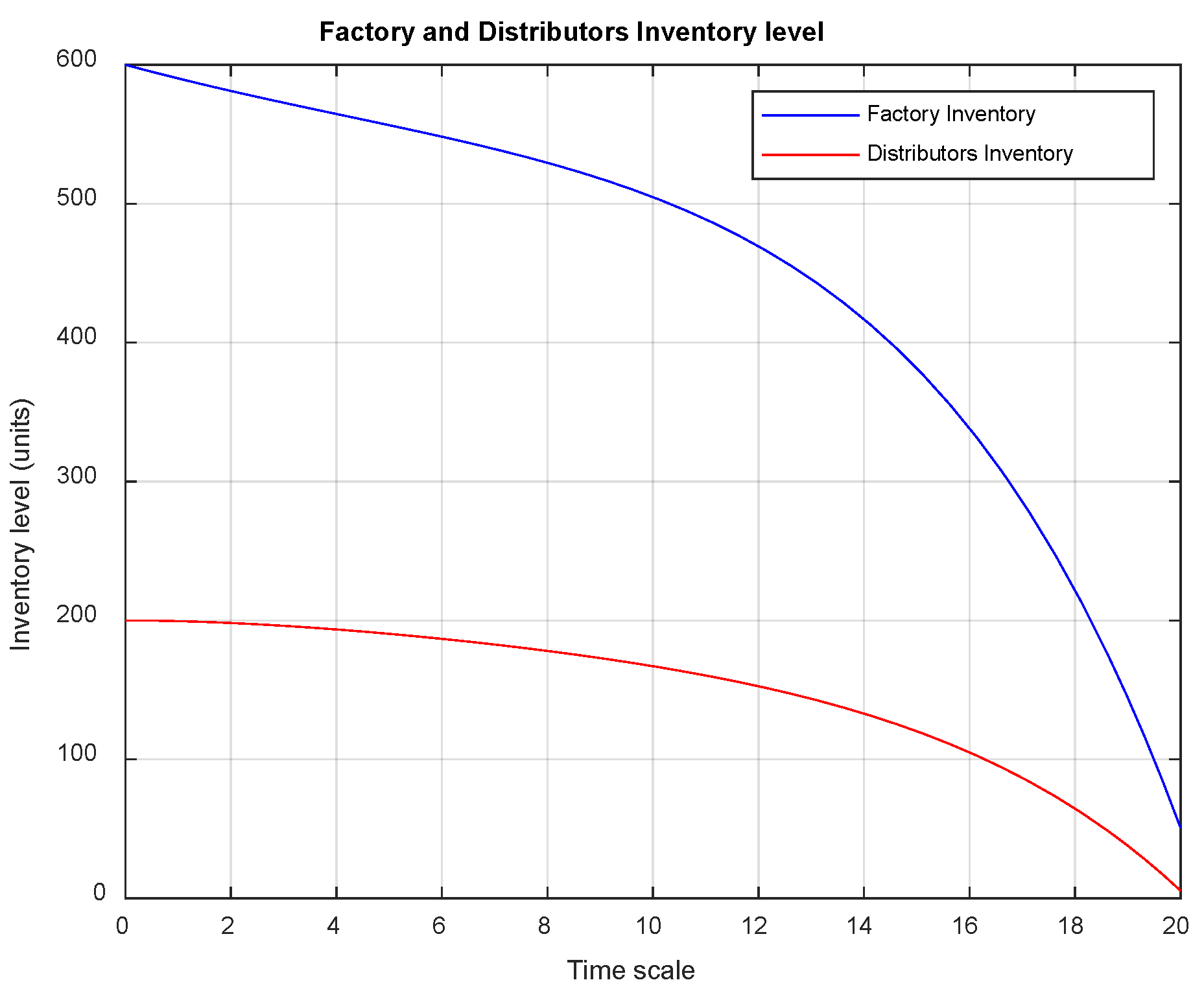
In Figure 4, the inventory level for factory and distributors is presented for a time horizon of 20 arbitrary units (au). It can be seen that factory inventory starts from a higher inventory level compared to distributors.
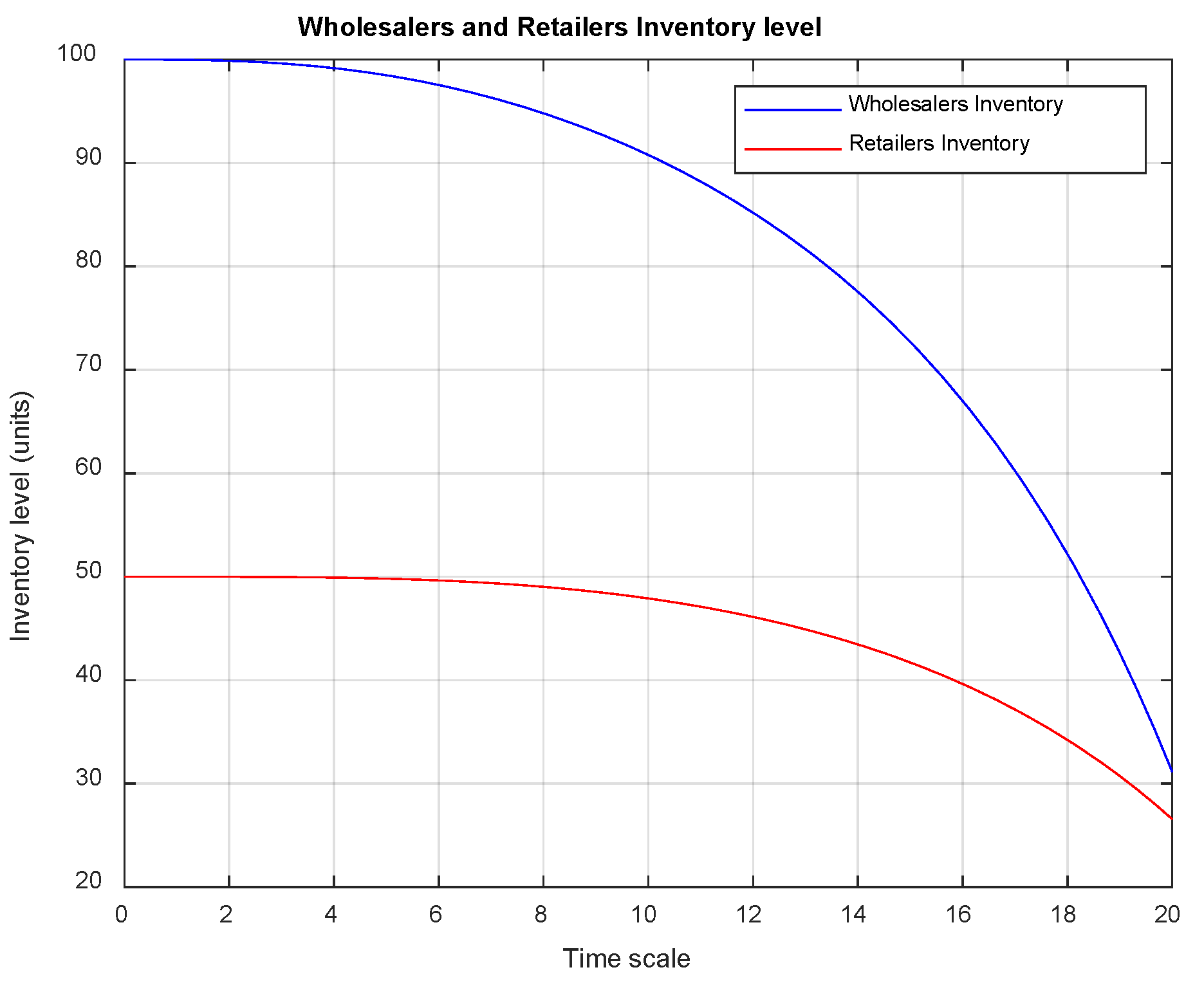
In Figure 5, an analysis of wholesaler and retailer inventory levels is presented considering a higher inventory level for wholesalers compared to retailers in a time horizon of 20 au.
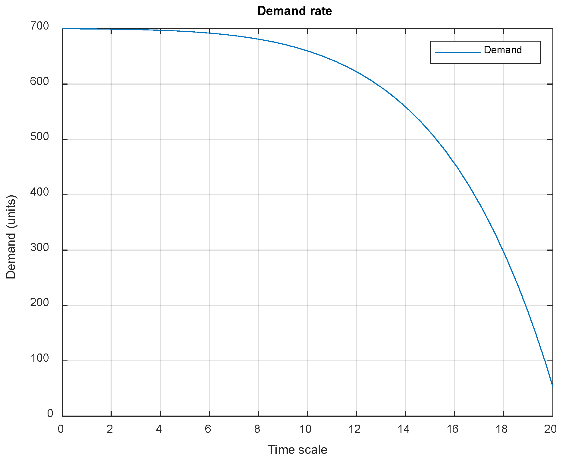
In Figure 6, a demand rate graph for a time horizon of 20 au is presented; considering time evolves to the final time horizon, the demand on the serial supply chain tends to be zero.

5.3. Sensitivity Analysis of R0

The variance in the state variable by the variation of a parameter is calculated through the sensitivity indices.
The sensitivity index on R0 is provided by:
α x R 0 = R 0 x · x R 0
where R0 is the reproductive number and x the parameter of interest
In order to calculate R0, we define from the Jacobian in Equation (34) the following relation:
R 0 = d e t J
Considering that the Jacobian is based on a linear system, the determinant of the Jacobian is the approach for the R0.
Based on this we have:
R 0 = φ 1 φ 2 φ 3 φ 4 C 1 C 2 C 3 C 4
Calculating the sensitivity index for φ1:
α φ 1 R 0 = R 0 φ 1 · φ 1 R 0
Recalling that, from Equation (33), we have: C 1 = 1 φ 1 .
After some manipulation, the sensitivity index for φ1 is:
α φ 1 R 0 = 1 C 1 φ 1
A similar procedure is developed in the sensitivity index for C1:
α C 1 R 0 = R 0 C 1 · C 1 R 0  
Which, after algebraic procedures, results in:
α C 1 R 0 = 1 C 1 φ 1  
We can see from Table 2 that the parameters that show the most sensitivity are the production rates compared to the sensitivity index of capacity levels.

6. Discussion

Dynamic supply chains present several advantages. In regard to system-dynamic approaches, the parameters of the mathematical model are capacity level and production rates. The manipulated variable is the demand, and the controlled variables are the inventory levels at each stage of the supply chain. The use of the mixing problem, or compartmental analysis, explores the balance between supply and demand along the supply chain. A sensitivity analysis was conducted, which give us an idea of the parameters that have more impact via the formulation of a sensitivity index. A proper stability analysis was conducted for a linear system. The application of energy-based optimal control for the dynamic supply chain was suitable. However, our interest is to extend these results, applying nonlinear model-predictive control approaches for a dynamic supply chain network. Furthermore, the option to develop data-driven control systems is a future goal for our research work.

7. Conclusions

Dynamic supply chains (SC) are important to regulate inventory, enable the balance of influx and outflux for materials, maximize profits, and minimize costs. In the context of HVM, the dynamic SC presents low variability and, therefore, can be modeled via ordinary differential equations, such as the mixing problem (compartmental analysis).
A serial supply chain was presented in which inventory levels are states of system dynamics, the input is the demand rate, and production rates are fixed parameters. An energy-based optimal control was analyzed in which the demand rate was optimized, subject to the system dynamics, via the Pontryagin maximum principle. The relation inventory level at each stage of the SC versus the demand presents a negative trend with a stable demand, as proposed in [40]. The demand profile takes into account that it is an independent demand, which implies that demand can be affected by trends and seasonal patterns. For an independent demand, the product-usage pattern is uniform and gradual.
Finally, an energy-based optimal control was developed for the system with proper simulations. As for future work, our aim is to extend these results for nonlinear systems via the application of nonlinear model predictive control, and also to extend these results via data driven control; previously, this was conducted through a systematic identification of data.

Author Contributions

Conceptualization, Y.A.D. and H.T.; methodology, H.T.; software, Y.A.D.; validation, Y.A.D. and J.S.-L.; formal analysis, J.S.-L.; investigation, Y.A.D.; resources, J.F.E.; writing—original draft preparation, Y.A.D. and J.S.-L.; writing—review and editing, H.T.; supervision, J.S.-L.; funding acquisition, H.T. and J.F.E. All authors have read and agreed to the published version of the manuscript.

Funding

This research received no external funding.

Conflicts of Interest

The authors declare no conflict of interest.

References

  1. Kappelman, A.C.; Sinha, A.K. Optimal control in dynamic food supply chains using big data. Comput. Oper. Res. 2021, 126, 105117. [Google Scholar] [CrossRef]
  2. Chen, P. The investment strategies for a dynamic supply chain under stochastic demands. Int. J. Prod. Econ. 2012, 39, 80–89. [Google Scholar] [CrossRef]
  3. Jain, V.; Deshmukh, S.G. Dynamic supply chain modeling using a new fuzzy hybrid negotiation mechanism. Int. J. Prod. Econ. 2009, 122, 319–328. [Google Scholar] [CrossRef]
  4. Jain, V.; Wadhwa, S.; Deshmukh, S.G. Revisiting information systems to support a dynamic supply chain: Issues and perspectives. Prod. Plan. Control Manag. Oper. 2009, 20, 17–29. [Google Scholar] [CrossRef]
  5. Umble, M.M. Analyzing manufacturing problems using V-A-T analysis. Prod. Inventory Manag. J. 1992, 33, 55–60. [Google Scholar]
  6. Eyers, D. Control architectures for industrial additive manufacturing systems. Proc. I MechE Part B J Eng. Manuf. 2018, 232, 1767–1777. [Google Scholar] [CrossRef]
  7. Orji, I.J.; Liu, S. A dynamic perspective on the key drivers of innovation-led lean approaches to achieve sustainability in manufacturing supply chain. Int. J. Prod. Econ. 2020, 219, 480–496. [Google Scholar] [CrossRef]
  8. Akyuz, G.A.; Erkan, T.E. Supply chain performance measurement: A literature review. Int. J. Prod. Res. 2018, 48, 5137–5155. [Google Scholar] [CrossRef]
  9. Singha, D.; Verma, A. Inventory management in supply chain. Mater. Today Proc. 2018, 5, 3867–3872. [Google Scholar] [CrossRef]
  10. De Vries, J. Diagnosing inventory management systems: An empirical evaluation of a conceptual approach. Int. J. Prod. Econ. 2007, 108, 63–73. [Google Scholar] [CrossRef]
  11. Fiestras-Janeiro, M.G.; García-Jurado, I.; Meca, A.; Mosquera, M.A. Cooperative game theory and inventory management. Eur. J. Oper. Res. 2011, 210, 459–466. [Google Scholar] [CrossRef]
  12. Bieniek, N. The ubiquitous nature of inventory: Vendor Managed Consignment Inventory in adverse market conditions. Eur. J. Oper. Res. 2019, 291, 411–420. [Google Scholar] [CrossRef]
  13. Duan, L.; Ventura, J.A. A dynamic Supplier Selection and Inventory Management Model for a Serial Supply Chain with a Novel Supplier Price Break Scheme and Flexible Time Periods. Eur. J. Oper. Res. 2019, 272, 979–998. [Google Scholar] [CrossRef]
  14. Giannoccaro, I.; Pontrandolfo, P.; Scozzi, B. A fuzzy echelon approach for inventory management in supply chains. Eur. J. Oper. Res. 2003, 149, 185–196. [Google Scholar] [CrossRef]
  15. Giannoccaro, I.; Pontrandolfo, P. Inventory management in supply chains: A reinforcement learning approach. Int. J. Prod. Econ. 2002, 78, 153–161. [Google Scholar] [CrossRef]
  16. Lieberman, M.B.; Helper, S.; Demeester, L. The empirical determinants of inventory levels in high-volume manufacturing. Prod. Oper. Manag. 1999, 8, 44–55. [Google Scholar] [CrossRef]
  17. Wiener, N. Cybernetics or Control and Communications in the Animal and the Machines; The MIT Press: Cambridge, MA, USA, 1948. [Google Scholar]
  18. Davizon, Y.A. Mathematical Modeling, Optimal Control and Stability Analysis for Dynamic Supply Chains. Ph.D. Thesis, The University of Texas at El Paso, El Paso, TX, USA, 2020. [Google Scholar]
  19. Song, D.P. Optimal integrated ordering and production policy in a supply chain with stochastic lead-time, processing-time, and demand. IEEE Trans. Autom. Control. 2009, 54, 2027–2041. [Google Scholar] [CrossRef]
  20. Kogan, K.; Lou, S.; Tapiero, C.S.; Shnaiderman, M. Supply chain with inventory review and dependent demand distributions: Dynamic inventory outsourcing. IEEE Trans. Autom. Sci. Eng. 2010, 7, 197–207. [Google Scholar] [CrossRef]
  21. Ignaciuk, P.; Bartoszewicz, A.A. Linear–quadratic optimal control strategy for periodic-review inventory systems. Automatica 2010, 46, 1982–1993. [Google Scholar] [CrossRef]
  22. Ignaciuk, P.; Bartoszewicz, A. Linear-Quadratic optimal control of periodic-review Perishable inventory systems. IEEE Trans. Control Syst. Technol. 2012, 20, 1400–1407. [Google Scholar] [CrossRef]
  23. Ivanov, D.; Dolgui, A.; Sokolov, B. Applicability of optimal control theory to adaptive supply chain planning and scheduling. Annu. Rev. Control 2012, 36, 73–84. [Google Scholar] [CrossRef]
  24. Ivanov, D.; Dolgui, A.; Sokolov, B. Robust dynamic schedule coordination control in the supply chain. Comput. Ind. Eng. 2016, 94, 18–31. [Google Scholar] [CrossRef] [Green Version]
  25. Ivanov, D.; Sethi, S.; Dolgui, A.; Sokolov, B. A survey on control theory applications to operational systems, supply chain management, and Industry 4.0. Annu. Rev. Control 2018, 46, 134–147. [Google Scholar] [CrossRef]
  26. Dolgui, A.; Ivanov, D.; Sethi, S.P.; Sokolov, B. Scheduling in production, supply chain and Industry 4.0 systems by optimal control: Fundamentals, state-of-the-art and applications. Int. J. Prod. Res. 2018, 57, 411–422. [Google Scholar] [CrossRef]
  27. Zu, Y.; Chen, L.; He, S. Inter-Organizational control of low-carbon production in a supply chain. IEEE Access 2019, 7, 170322–170332. [Google Scholar] [CrossRef]
  28. Wu, Z. Optimal control approach to advertising strategies of a supply chain under consignment contract. IEEE Access 2019, 7, 41454–41462. [Google Scholar] [CrossRef]
  29. Wu, Z.; Chen, D. New optimal-control-based advertising strategies and coordination of a supply chain with differentiated products under consignment contract. IEEE Access 2019, 7, 170703–170714. [Google Scholar] [CrossRef]
  30. Yu, H.; Bai, S.; Chen, D. An optimal control model of the low-carbon supply chain: Joint emission reduction, pricing strategies, and new coordination contract design. IEEE Access 2020, 8, 106273–106283. [Google Scholar] [CrossRef]
  31. Rarità, L.; Stamova, I.; Tomasiello, S. Numerical schemes and genetic algorithms for the optimal control of a continuous model of supply chains. Appl. Math. Comput. 2021, 388, 125464. [Google Scholar] [CrossRef]
  32. He, Y.; Zheng, S.; Yuan, L. Dynamics of Fractional-Order Digital Manufacturing Supply Chain System and Its Control and Synchronization. Fractal Fract. 2021, 5, 128. [Google Scholar] [CrossRef]
  33. Kegenbekov, Z.; Jackson, I. Adaptive Supply Chain: Demand–Supply Synchronization Using Deep Reinforcement Learning. Algorithms 2021, 14, 240. [Google Scholar] [CrossRef]
  34. Badillo, I.; Tejeida, R.; Morales, O.; Flores, M. Supply Chain Management from a Systems Science Perspective, Supply Chain Management—New Perspectives; Intech.: London, UK, 2011. [Google Scholar]
  35. Zill, D.G. Advanced Engineering Mathematics, 6th ed.; Jones & Bartlett Learning: Burlington, MA, USA, 2017. [Google Scholar]
  36. Herty, M.; Ringhofer, C. Feedback controls for continuous priority models in supply chain management. Comput. Methods Appl. Math. 2011, 11, 206–213. [Google Scholar] [CrossRef] [Green Version]
  37. Martinez-Luaces, V. Square Matrices Associated to Mixing Problems ODE Systems. Matrix Theory—Applications and Theorems; Hassan, A.Y., Ed.; Intech.: London, UK, 2018. [Google Scholar]
  38. Bassingthwaighte, J.B.; Butterworth, E.; Jardine, B.; Raymond, G.M. Compartmental Modeling in the Analysis of Biological Systems. In Toxicology: Volume I, Methods in Molecular Biology; Springer: Berlin/Heidelberg, Germany, 2012; Volume 929. [Google Scholar]
  39. Rahimian, E.; Zabihi, S.; Mahmood Amiri, M.; Linares-Barranco, B. Digital implementation of the two-compartmental Pinsky–Rinzel pyramidal neuron model. IEEE Trans. Biomed. Circuits Syst. 2018, 1, 47–57. [Google Scholar] [CrossRef] [PubMed]
  40. Fogarty, D.W.; Blackstone, J.H.; Hoffmann, T.R. Production & Inventory Management; South-Western Publishing Company: Nashville, TN, USA, 1991. [Google Scholar]
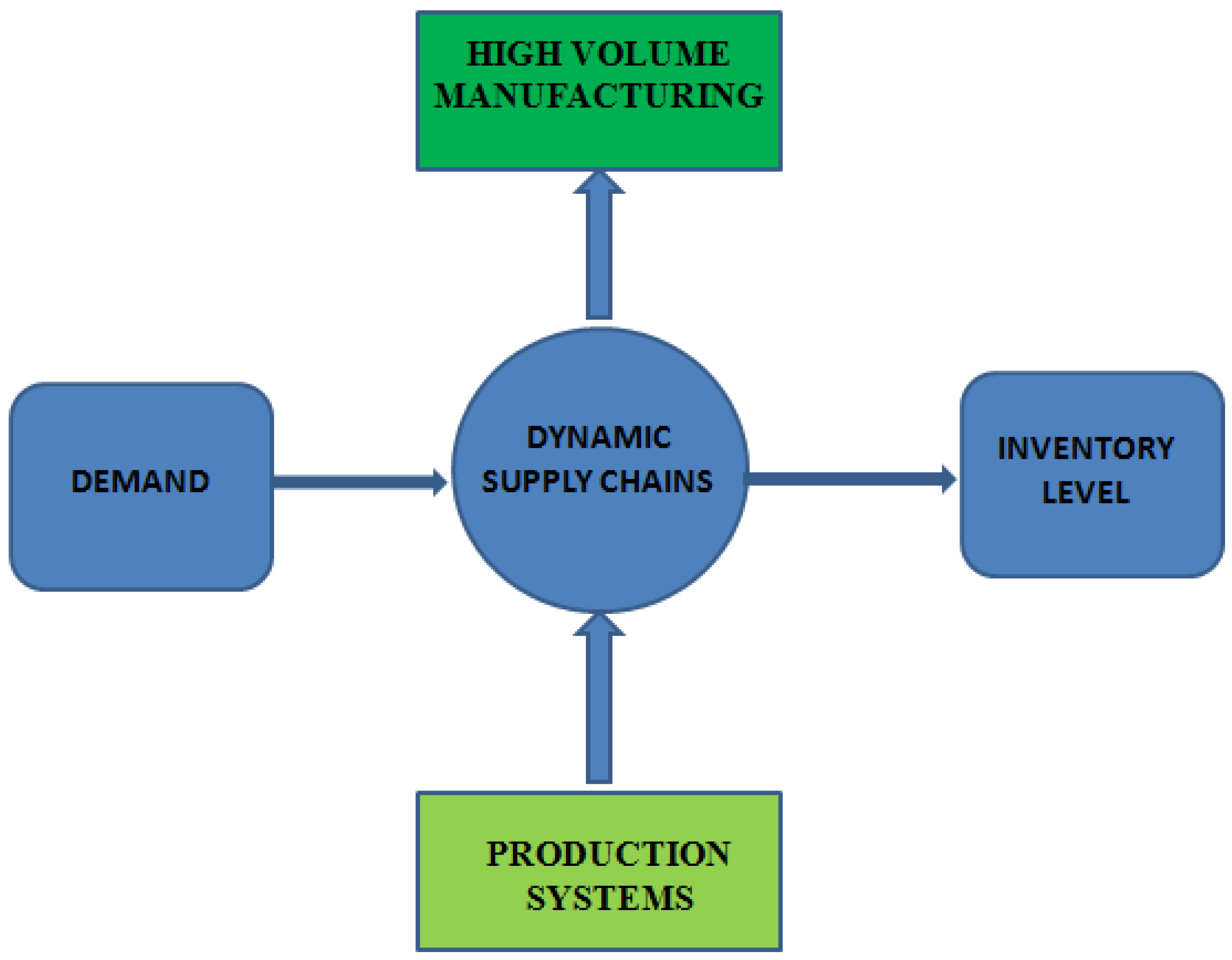
Figure 1. Dynamic supply chains.
Applsci 12 05347 g001
Figure 2. Model-based control systems (adapted from [18]).
Applsci 12 05347 g002
Figure 3. Generic four-echelon serial SC realization for a capacity–inventory management model.
Applsci 12 05347 g003
Figure 4. Factory and distributor inventory levels.
Applsci 12 05347 g004
Figure 5. Wholesaler and retailer inventory levels.
Applsci 12 05347 g005
Figure 6. Demand rate.
Applsci 12 05347 g006
Table 1. Relevant optimal control for supply chains; literature review from 2016 to 2021.
ManuscriptContributionControl Approach
Ivanov, et al., 2016, [24]This paper addresses the problem of supply chain coordination with a robust schedule coordination approach, applying optimal control theory.Optimal control
Ivanov, et al., 2018, [25]This research work extends a previous survey by identifying two new directions for control theory applications and digital technology use in control-theoretic models.Optimal control
Dolgui, et al., 2018, [26]A survey on optimal control applications regarding scheduling in production, supply chain, and Industry 4.0 systems via deterministic maximum principle.Optimal control
Zu, et al., 2019, [27]This paper presents a method to study the Stackelberg differential game between a manufacturer and a supplier.Differential game
Wu, 2019, [28]This paper presents a differential game for a single manufacturer and a single retailer in a supply chain under a consignment contract.Optimal control
Wu and Chen, 2019, [29]The cooperative advertising problem is addressed, applying optimal control theory for a supply chain under a consignment contract in a competitive environment.Optimal control
Yu, et al., 2020, [30]An optimal control model is presented for a class of low-carbon supply chain system. A linear differential equation describes the dynamics of emission reduction level.Optimal control
Rarita, et al., 2021, [31]This paper considers supply chains modeled by partial and ordinary differential equations.Optimal control
He, et al., 2021, [32]In this paper, a fractional-order digital manufacturing supply chain system is proposed with feedback controllers to control the chaotic supply chain system.Fractional order control
Kegenbekov and Jackson, 2021, [33]This paper shows how a deep reinforcement learning-based optimization algorithm can synchronize inbound and outbound flows to support a business operating in the stochastic environment.Deep reinforcement learning
Table 2. Sensitivity indices of R0 corresponding to all parameters.
ParameterValueSensitivity Index
Φ1100.001
Φ2100.001
Φ3100.001
Φ4100.001
C1100−0.001
C2100−0.001
C3100−0.001
C4100−0.001
Publisher’s Note: MDPI stays neutral with regard to jurisdictional claims in published maps and institutional affiliations.