Abstract
Vibrational spectroscopies provide information about the biochemical and structural environment of molecular functional groups inside samples. Over the past few decades, Raman and infrared-absorption-based techniques have been extensively used to investigate biological materials under different pathological conditions. Interesting results have been obtained, so these techniques have been proposed for use in a clinical setting for diagnostic purposes, as complementary tools to conventional cytological and histological techniques. In most cases, the differences between vibrational spectra measured for healthy and diseased samples are small, even if these small differences could contain useful information to be used in the diagnostic field. Therefore, the interpretation of the results requires the use of analysis techniques able to highlight the minimal spectral variations that characterize a dataset of measurements acquired on healthy samples from a dataset of measurements relating to samples in which a pathology occurs. Multivariate analysis techniques, which can handle large datasets and explore spectral information simultaneously, are suitable for this purpose. In the present study, two multivariate statistical techniques, principal component analysis-linear discriminate analysis (PCA-LDA) and partial least square-discriminant analysis (PLS-DA) were used to analyse three different datasets of vibrational spectra, each one including spectra of two different classes: (i) a simulated dataset comprising control-like and exposed-like spectra, (ii) a dataset of Raman spectra measured for control and proton beam-exposed MCF10A breast cells and (iii) a dataset of FTIR spectra measured for malignant non-metastatic MCF7 and metastatic MDA-MB-231 breast cancer cells. Both PCA-LDA and PLS-DA techniques were first used to build a discrimination model by using calibration sets of spectra extracted from the three datasets. Then, the classification performance was established by using test sets of unknown spectra. The achieved results point out that the built classification models were able to distinguish the different spectra types with accuracy between 93% and 100%, sensitivity between 86% and 100% and specificity between 90% and 100%. The present study confirms that vibrational spectroscopy combined with multivariate analysis techniques has considerable potential for establishing reliable diagnostic models.
1. Introduction
Over the past decades, various works have been published to promote the use of vibrational spectroscopy as a diagnostic tool in clinical practice, with the role of a complementary technique to support the results obtained by means of conventional histological and cytological analysis techniques [1,2,3,4,5,6]. The two main vibrational techniques are Raman and Fourier Transform Infrared (FTIR) spectroscopies, which both are able to provide information about the different types of functional groups and their relative content inside the investigated cell or tissue samples [7,8]. In particular, in both cases the sample is excited by means of a radiation beam and the spectral intensity of the inelastically scattered (Raman) or absorbed (FTIR) radiation from different biological macromolecules (nucleic acids, proteins, lipids, etc.) is detected. However, vibrational spectra measured from normal and pathological samples are often similar to each other, due to the fact that spectral features related to specific cellular components only slightly change as a result of chemical–physical stress or the onset of pathology. So, the visual inspection of the measured spectrum in most cases is not enough to make a reliable diagnosis.
Such a problem can be addressed by collecting many spectra from the investigated samples and by analysing them through multivariate statistical methods. Multivariate analysis of the measured spectra is a critical step for data interpretation and the possibility of providing a reliable diagnostic result [9]. Multivariate techniques have proved to be an efficient tool for obtaining information about large datasets of spectral measurements, each one consisting of many variables which are the scattered (as for Raman) or absorbed (as for FTIR) radiation intensity at hundreds of wavenumber values [10]. In fact, these methods allow the visualization of similarities and differences in the data and to build classification models which can be used to predict the class of unknown samples of the same type: consequently, they are very promising as diagnostic tools.
The multivariate analysis techniques can be divided into unsupervised and supervised methods. The former aim to detect similarities and differences inside a dataset comprising spectra of different classes when there is no information available regard to the class to which they belong. Principal Component Analysis (PCA) is the most popular unsupervised method [11]. On the contrary, supervised methods label the classes to be differentiated. They are based on two successive steps: firstly, samples whose class is known are used to build a model with proper parameters that optimize the discrimination between the data from different classes; then, unknown samples are assigned to a suitable class using the parameters optimized during the first step. Linear Discriminant Analysis (LDA) and Partial Least Squares Discriminant Analysis (PLS-DA) are effective supervised methods [11].
Principal Components Analysis (PCA) is one of the most powerful multivariate techniques used for exploratory data analysis, i.e., it provides preliminary approaches to find differences and similarities among data. In the case of spectroscopy investigation, the data are the spectra measured from different samples. All the measured spectra can be represented as a dataset or matrix X, with n rows, corresponding to the measured samples, and m columns, each one corresponding to the spectral signal for a specific wavenumber value. The first aim of PCA is to reduce the dimensionality of large datasets (those including all the values of spectral variables in a wide wavenumber range for all the measured samples). The dimensionality reduction is performed by finding new variables, that are linear functions of those of the original dataset, that successively maximize variance and that are uncorrelated with each other [12]. Briefly, PCA transforms the m original variables, consisting of the signal values for the m wavenumber values, into a new set of m variables, called principal components (PCs), each one is a linear combination of the m original variables. Each original spectrum takes specific values in the set of PCs: such values are called scores. The criterion according to which the first PC is chosen is that it contains most of the variance of the scores, and each subsequent PC contains less variance. A score plot, reporting the score values of two different PCs for all the n samples, allows for visualizing differences and similarities among the n samples, based on the original spectral characteristics. The coefficients describing the influence of the original variables on the score values for a given PC are known as loadings: they give information about the wavenumber values at which the spectral signals furnish the main variability inside the dataset, corresponding to changes in the molecular components contributing to the spectra. In fact, many works reported the discrimination of vibrational spectra from biological samples of different types through PCA score plots as well as the identification of differences in their biochemical content through the main spectral features of the loading plots [13,14,15,16].
LDA is a supervised classification method which can be used to classify objects (such as spectra measured from unknown samples) as belonging to classes which have been specified before the model is created [11]. In particular, LDA is based on a linear transformation of m variables describing n samples belonging to different classes, so that samples from the same class are close together but samples from different classes are far apart from each other. This goal is achieved by means of a mathematical classification algorithm (based on a Mahalanobis distance calculation between the samples for each class) which maximizes the distance between the means of the classes while minimizing the variance within each class. So, a predicted class is assigned to each sample. After the classification model has been built, it is later used for allocating new and unknown samples to the most probable class. However, the LDA method cannot be applied when the number of spectral variables is larger than the number of samples (m < n) [17]. This issue can be solved by calculating PCA for the spectral data prior to LDA and applying LDA to the PCA scores: this is how the PCA-LDA algorithm works.
N. Iturrioz-Rodriguez et al. showed that Raman spectroscopy can identify changes in the molecular composition of healthy astrocytes compared to glioblastoma patient-derived cells and that, associated with PCA-LDA, can become a diagnostic tool with accuracy values between 80% and 100% [18]. PCA-LDA statistics were also used to classify oral squamous cell carcinoma cells in saliva samples with an accuracy of 90%, in the case of the Raman data set, and 82%, for the FT-IR one [19]. The PCA-LDA model also has been demonstrated to yield 100% classification accuracy to differentiate FTIR spectra from hepatitis C infected and healthy freeze-dried sera samples [20]. The PCA-LDA discrimination model correctly classified also FTIR spectra from gynaecological cancer samples into malignant and benign groups with accuracies of 96% and 93% for the k-fold and “leave one out” validation schemes, respectively [21].
PLS-DA is a supervised classification technique which combines partial least squares (PLS) regression with LDA. Firstly, a PLS model is built from the spectral data (X matrix) and a dependent variable describing the class of spectra (Y matrix), so that Y = XB + E, where B is a matrix of regression coefficients and E is a matrix of residuals. The X matrix consists of n rows, each one related to a sample, and m columns, each one related to the signal intensity for each wavenumber value, whereas the Y matrix consists of n rows, each one is a categorical variable that specifies the type of sample (samples of different type are described by different discrete numbers that encode the class membership, as −1 and +1). Such a PLS model, that relates the variations of the spectral data to the class of cells from which the spectra were measured, firstly transforms the original spectral variables into a set of a few latent variables (LVs), called factors. Then these new variables are used for regression with the dependent variable [11,22]. In the PLS models, scores and loadings specify how the samples and variables are projected along the factors. In particular, PLS scores, similarly to PCA scores, are the sample coordinates along the model components: they are computed in such a way that they capture the part of the structure in X which is most predictive for Y. The PLS loadings specify how much each X-variable contributes to a specific model component, in the same way as the PCA loadings do. A two-dimensional scatter plot of scores for two specified factors gives information about patterns in the samples, i.e., the closer the samples are in the scores plot, the more similar they are with respect to the two components concerned, whereas distant samples in the score plot are different. The corresponding loadings plot provides information about which variables are responsible for differences between samples. In addition, the regression coefficients determine what is the weight of each variable when predicting a particular Y response, i.e., variables with a large regression coefficient play an important role in the regression model. A positive coefficient shows a positive link with the response, and a negative coefficient shows a negative link. The difference between loadings and regression coefficients is that the former is related to each LV, whereas the latter refers to a model with a specific number of LVs. After the PLS regression model has been built, a linear discriminant classifier is used for classifying unknown samples (spectra). When −1 and +1 are the encoded values of class membership, if the predicted value is above 0, a corresponding object is considered a member of a class and if not it is considered a stranger.
Recently, PLS regression algorithms have been widely used in the biomedical field to construct predictive models based on Raman and FTIR spectral signals. R. Pinto Aguiar et al. classified Raman spectra from brain tissue using PLS-DA discrimination into normal (cerebellum and meninges) and tumours (glioblastoma, medulloblastoma, schwannoma, meningioma) with an accuracy of 94.1% [23]. Raman spectroscopy was also used by D. Cullen et al. to investigate lymphocytes of patients with late radiation toxicity following radiotherapy treatment because of prostate cancer: the PLS-DA model developed to classify patients using known radiation toxicity scores achieved an accuracy value of 93% [24]. X. Yang et al. reported PLS-DA results about first derivative FTIR data in nucleic acids spectral range collected from serum samples of patients with lung cancer and healthy people: they achieved 87.10% accuracy for discrimination of the two types of samples [25]. FTIR and PLS-DA were also used to develop a prediction model based on the spectra of blood serum samples collected from healthy people and patients affected by attention deficit and hyperactivity disorder: the model was able to distinguish ADHD patients from healthy individuals with an accuracy of 100% [26].
Overall, these two different classification models can have different performances when applied to the same dataset for diagnostic purposes. Therefore, it is important to compare the predicted results of both models in order to optimize the diagnostic phase. Hence, the aim of the present study is to evaluate and compare the performance parameters of the PCA-LDA and PLS-DA models for the class prediction of three different datasets of vibrational spectra: a simulated dataset and two experimental datasets of Raman and FTIR spectra, respectively. The comparison is performed by evaluating the values of accuracy, sensitivity and specificity obtained in the class prediction for a subset of each of the three datasets, used as a test set. The obtained results point out that both the classification models were able to predict the class of the different spectra with high values of accuracy (93% ÷ 100%), sensitivity (86% ÷ 100%) and specificity (90% ÷ 100%). So, if datasets of different types of spectra are available, the application of both classification models to the prediction of the class of unknown measured spectra is promising as a reliable complementary diagnostic tool in the clinical setting.
2. Materials and Methods
2.1. Simulated Spectra
Vibrational spectra were simulated by overlapping several Gaussian functions. In particular, a basic simulated vibrational spectrum yR was built, in the 750–1750 cm−1 spectral range, by means of 15 component functions yi, as described by the following equation:
where Ai, x0i and σi are the amplitude, wavenumber and broadening parameters, respectively, of each yi. The values assigned to such parameters are reported in Table S1. In particular, the relative intensity, spectral wavenumber and broadening of each yi have been chosen in order to yield a yR spectrum similar to a typical vibrational spectrum measured from a cellular sample. Such simulated function yR can be considered to be a model of spectrum measured for a control-like sample. In addition, the Ai values corresponding to the peak centred at 785, 830, 1090 and 1580 cm−1 have been decreased by 10% with respect to the corresponding values of the control-like spectrum, in order to simulate a basic exposed-like spectrum.
Starting from the basic spectra, 25 different spectra were obtained for the two types of samples (control-like and exposed-like), by randomizing the values of Ai of each single peak in a ±10% range of values reported in Table S1.
Each of these 50 single simulated spectra was area normalized, i.e., the intensity value corresponding to each wavenumber value was divided by the total intensity of the spectrum. The basic Raman spectra were calculated by means of SigmaPlot software (version 12.5, Systat Software).
2.2. Measured Spectra
Three different cellular models were chosen to confirm the results obtained for simulated spectra:
- MCF10A cells, as a model of a normal breast cellular line. These cells were exposed to proton beam radiation with a dose of 4 Gy, which causes cellular damage involving nucleic acid and DNA/RNA components, as reported in [27]. Unexposed cells were considered as a control sample. Both control and exposed cells were measured by means of a Raman confocal micro-spectrometer apparatus (Labram from Jobin–Yvon Horiba) and the Raman spectra were pre-processed as described in [27]. Briefly, Raman spectra were measured for about 30 randomly chosen single cells grown on coverslip slides; each cell was excited by the 514.5 nm line from an Ar ion laser with about 10 mW power, which was focused, by means of a 100x oil immersion objective, on the cell nucleoplasm region; three acquisitions of 10 s each was averaged to produce each Raman spectrum. The Raman scattered signal was analysed, in backscattering geometry, by a spectrometer equipped with a 600 grooves/mm grating and it was detected by a charged coupled device cooled at 223 K.
- MCF7 and MDA-MB-231, as a model of malignant non-metastatic (MCF7) and metastatic (MDA-MB-231) breast cancer cell lines. The FTIR spectra of such cells were measured in transflection mode by means of an FTIR Microscope HYPERION 2000 connected to a Vertex 70 Bruker interferometer (Bruker Optik GmbH), as described in [28]. Briefly, each FTIR spectrum was recorded, using a 15× objective, in the 1000–4000 cm−1 spectral range with the resolution of 4 cm−1 and 64 scans. The sampling area was about 80 × 80 μm in size, including 3–4 cells of each type. The absorption signal was detected with an MCT (mercury cadmium telluride) detector (cooled to liquid N2 temperature). For each experiment, about 30 cells were measured.
2.3. Data Analysis
In order to evaluate the classification models, each of the three different groups of spectra was separated into a calibration set and a test set, comprising, respectively, about 70% and 30% of the total number of spectra of each group. The spectra assigned to the test group were randomly chosen using a random number generator.
Exploratory data analysis was performed for each calibration set by means of PCA, in order to visualize in the score plots the separation of the two different classes of samples and the spectral variables to which this separation is related. Full cross-validation was used to validate the PCA results.
Classification models for discriminating samples from the two classes of each group were built by using the PCA-LDA and PLS-DA techniques for the calibration set, whereas the test set is used to evaluate the model classification performance, that is the obtained values of accuracy, sensitivity and specificity. Accuracy corresponds to the total number of samples correctly classified considering true and false negatives, sensitivity assesses the ability of the test to classify positive cases (e.g., cases with disease) while specificity is a measure of the ability of the test to identify negative cases (e.g., cases without disease).
All chemometric analyses were performed with the Unscrambler X CAMO software (version 10.4), whereas t-test analysis was performed by SigmaPlot software (version 12.5, Systat Software, San Jose, CA, USA).
3. Results and Discussion
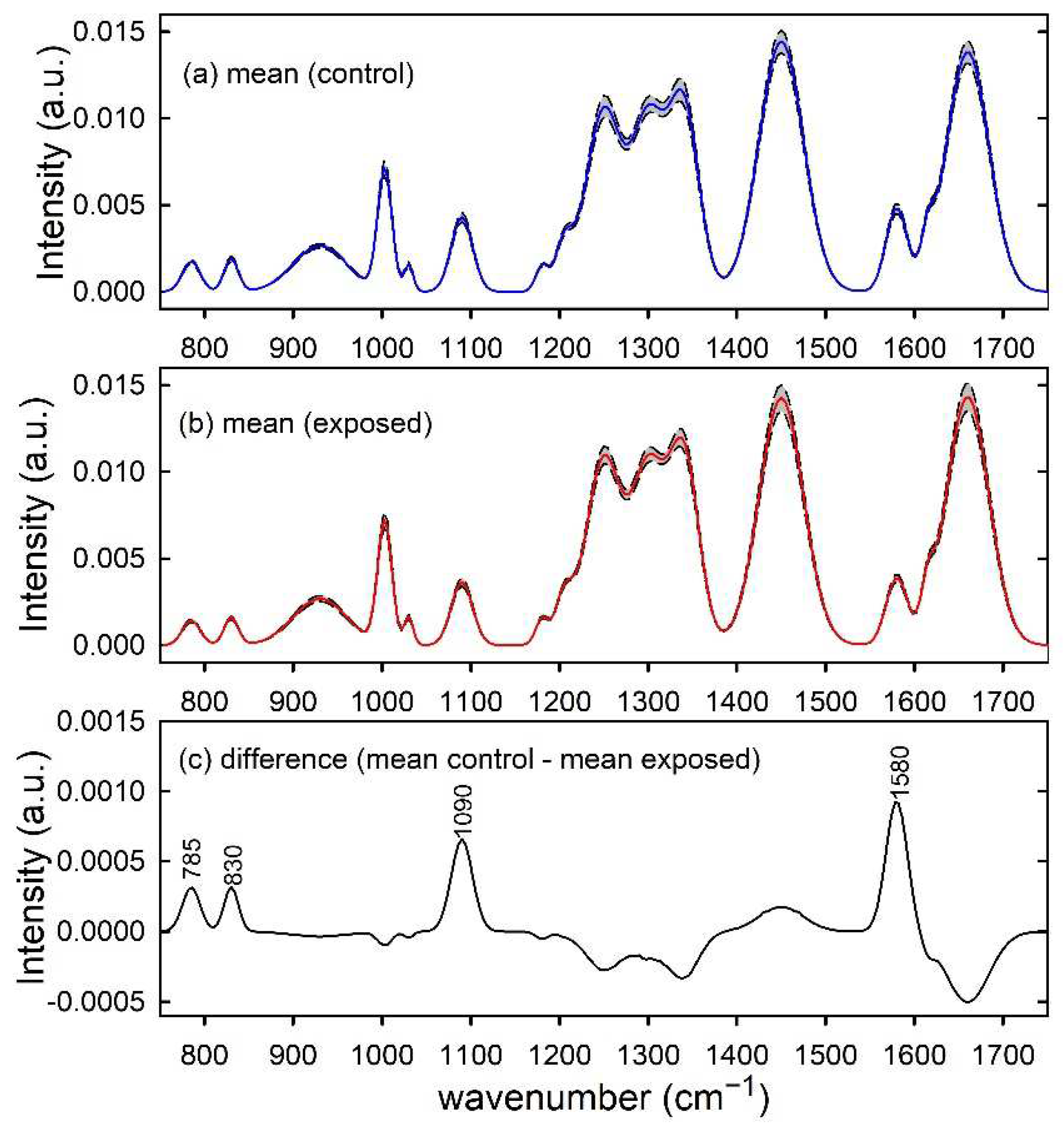
The normalized simulated spectra of control-like and exposed-like types were independently averaged in order to obtain mean spectra, which are shown in Figure 1a,b, respectively. As expected, the difference between control and exposed mean spectra, shown in Figure 1c, is characterized by large positive peaks centred at 785, 830, 1090 and 1580 cm−1, corresponding to the spectral peaks whose intensity has been decreased for the basic spectrum in order to simulate damage in exposed-like type spectrum. The other positive and negative peaks in Figure 1c are related to random intensity differences that affect the mean spectra and they are particularly relevant for the largest intensity features, as those centred at 1450 cm−1, 1660 cm−1 and 1200–1400 cm−1 spectral range.
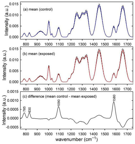
Figure 1.
Synthetic spectra modelling control (a) and exposed (b) samples. The mean spectra are reported by blue and red lines in (a,b), respectively. Standard deviation spectra are also reported as dashed lines and the grey area corresponds to spectral values between mean ± standard deviation values. The spectral differences between mean values are reported in (c) and the wavenumber values of spectral features mainly contributing to such a difference are labelled for clarity.
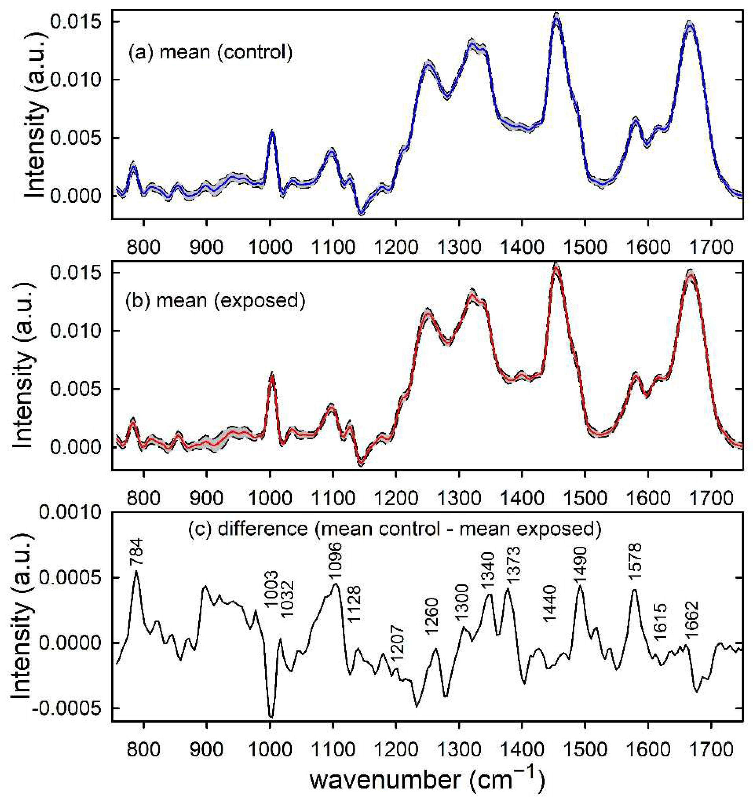
Similarly, the normalized mean Raman spectra of unexposed and proton-exposed MCF10A cells are plotted in Figure 2a,b, respectively. Such spectra are characterized by Raman peaks and spectral features related to the main cellular components, as nucleic acids (784, 1096, 1340, 1373, 1490 and 1578 cm−1), proteins (1003, 1032, 1128, 1207, 1260, 1340, 1615 and 1662 cm−1) and lipids (1128, 1300 and 1440 cm−1) [29]. The positive peaks in the difference spectrum in Figure 2c suggest that the main effect of radiation exposure on the Raman spectra consists in a relative decrease of nucleic acid components, as a consequence of larger exposure damage to DNA/RNA than to protein and lipid components [27]. A significant intensity decrease of the Raman peaks related to the phosphodiester bond (at 784 cm−1) and DNA bases ring modes (at 1574 cm−1) was also reported by Synytsya et al. in proton irradiated calf thymus DNA [30]. Modification of the above Raman peak related to nucleic acids was also reported by K. Sofinska et al. for cellular samples exposed to different types of ionizing radiation, such as proton and γ-rays [31].
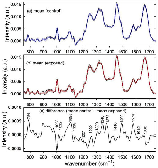
Figure 2.
Raman spectra of control (a) and proton-exposed (b) MCF10A cells. The mean spectra are reported by blue and red lines in (a,b), respectively. Standard deviation spectra are also reported as dashed lines and the grey area corresponds to spectral values between mean ± standard deviation values. The spectral differences between mean values are reported in (c) and the wavenumber values of spectral features mainly contributing to such a difference are labelled for clarity.
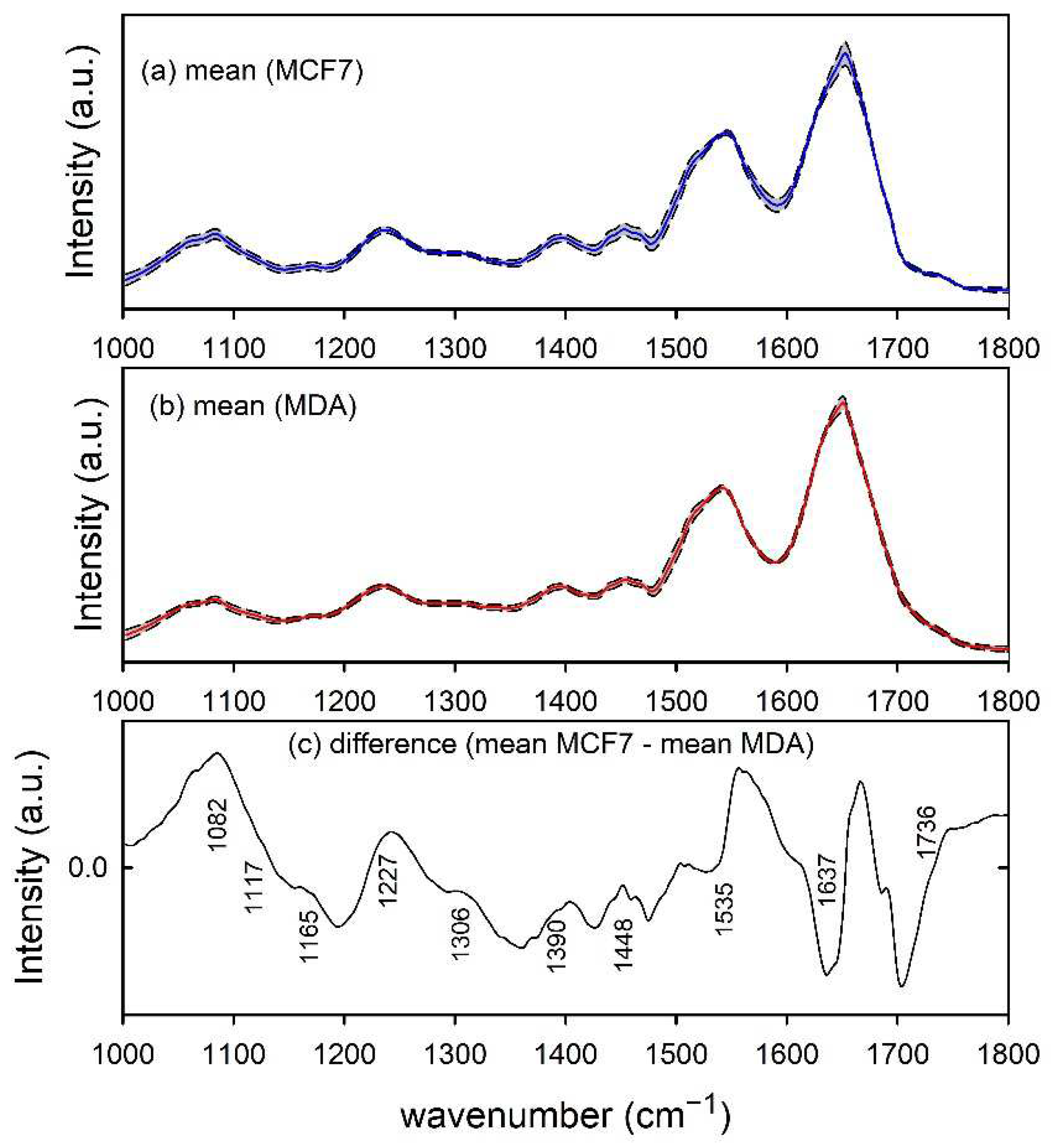
Furthermore, the infrared absorption spectra of MCF7 and MDA cells, shown in Figure 3a,b, respectively, are characterized by spectral peaks and bands related to nucleic acids (1082, 1117 and 1227 cm−1), proteins (1165, 1306, 1390, 1448, 1535 and 1637 cm−1) and lipids (1390, 1448 and 1736 cm−1). The difference spectrum in Figure 3c indicates that the two types of cells can be biochemically discriminated according to the larger relative amount of nucleic acid content in MCF7 cells with respect to MDA ones, as suggested by the spectral peak at 1082 and 1227 cm−1, whereas the peaks at about 1535 and 1637 cm−1 are due to a relative spectral shift of the amide II and I band for the two types of cell [28]. Both such results are in good agreement with those reported in the literature. In particular, both Talari et al. [32] and Abramczyk et al. [33] found a larger relative amount of nucleic acids in the MCF7 cells with respect to MDA cells. As for the shifts of amide I and II bands, they might be connected with changes in the secondary protein structures occurring during the process of carcinogenesis [28].
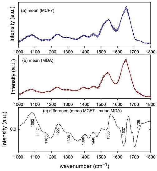
Figure 3.
FTIR spectra of MCF7 (a) and MDA (b) cells. The mean spectra are reported by blue and red lines in (a,b), respectively. Standard deviation spectra are also reported as dashed lines and the grey area corresponds to spectral values between mean ± standard deviation values. The spectral differences between mean values are reported in (c) and the wavenumber values of spectral features mainly contributing to such a difference are labelled for clarity.
The difference plots indicate that, for all three cases, important intensity differences between the mean spectra of two types of cells characterize the investigated range. In order to show whether these spectral differences would be enough to discriminate and classify the two types of cells, we firstly analysed data by means of the PCA technique. In particular, samples from the calibration sets were analysed by PCA, using a full cross-validation method. Although PCA is not able to provide classification, it is largely used for data interpretation and visualization, as well as to reduce dimension by extracting information from high-dimension data to project them into a lower dimension. In particular, PCA score plots are able to visualize the similarity and differences between samples and PCA loading plots provide information about the spectral variables responsible for the differences.
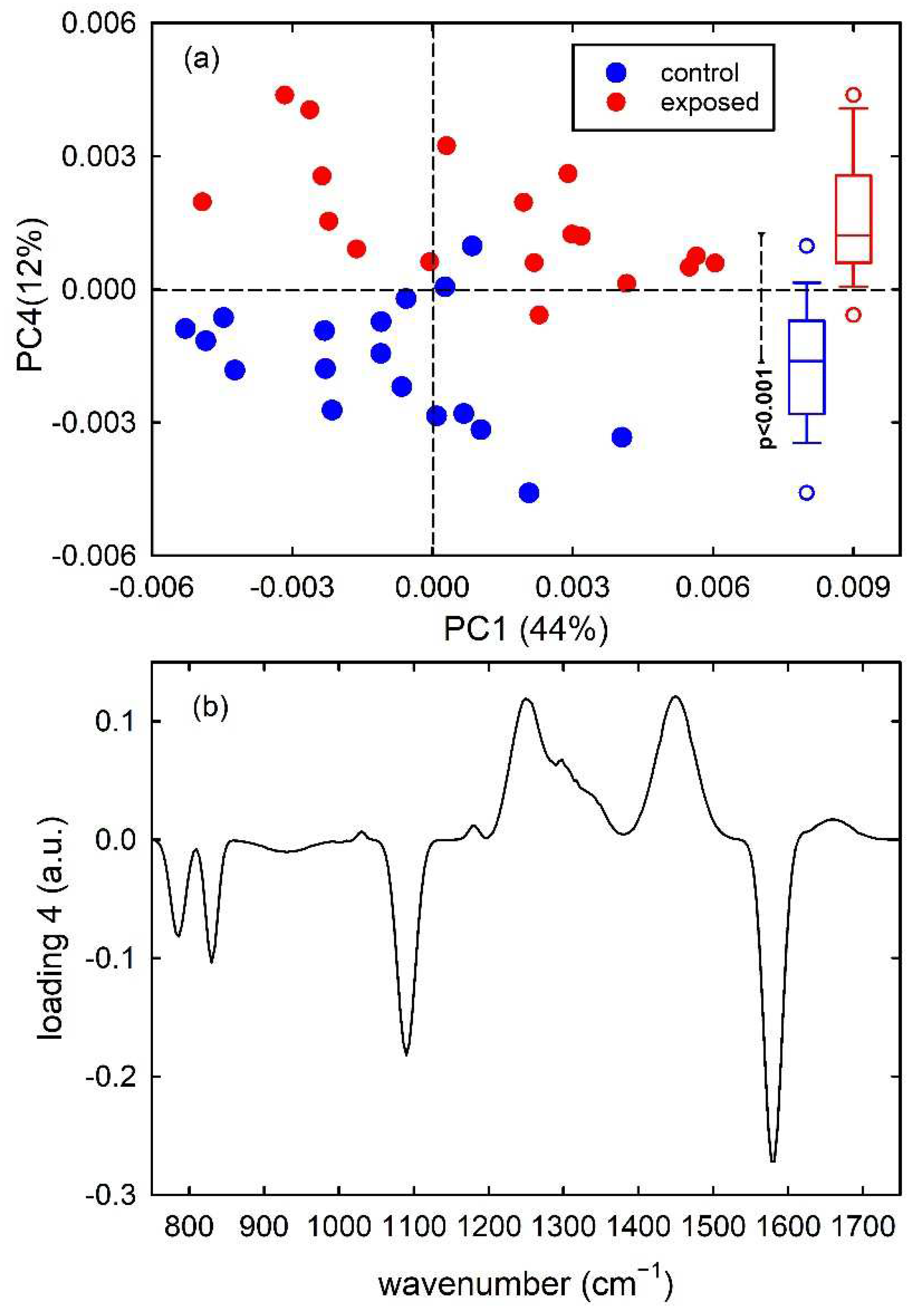
Figure 4a shows the score plots of PC1/PC4, with the percentage of each PC in the axis, for the simulated dataset. It has been verified that the first 7 principal components carried around 99% of all the spectral variation found in the dataset. As is visible in the score plot, the PC4 provides the main contribution to the discrimination of control-like spectra from exposed-like ones. In particular, control-like spectra have negative PC4 values and exposed-like spectra are characterized by positive PC4 values, with minor overlap. The results of the t-test analysis performed for the distributions of PC4 score values for the two types of spectra prove that they are significantly different, as deduced from the box plots on the right side of Figure 4a. The representation of the loadings of PC4 in Figure 4b points out four intense negative peaks (at 785, 830, 1090 and 1580 cm−1) whose spectral positions correspond to those of the four positive peaks in the difference of mean spectra shown in Figure 1c. Therefore, PCA confirms that the two types of spectra can be mainly discriminated according to PC4 and such discrimination is related to the simulated spectral peaks whose intensity was changed to differentiate between control-like and exposed-like spectra.

Figure 4.
PC4 vs. PC1 score plot (a) for the synthetic control (blue dots) and exposed (red dots) vibrational spectra. The box plots of the PC4 score values are shown on the right side of (a): the results of the t-test point out that the two distributions of score values are significantly different (p < 0.001). Loading 4 spectrum is reported in (b).
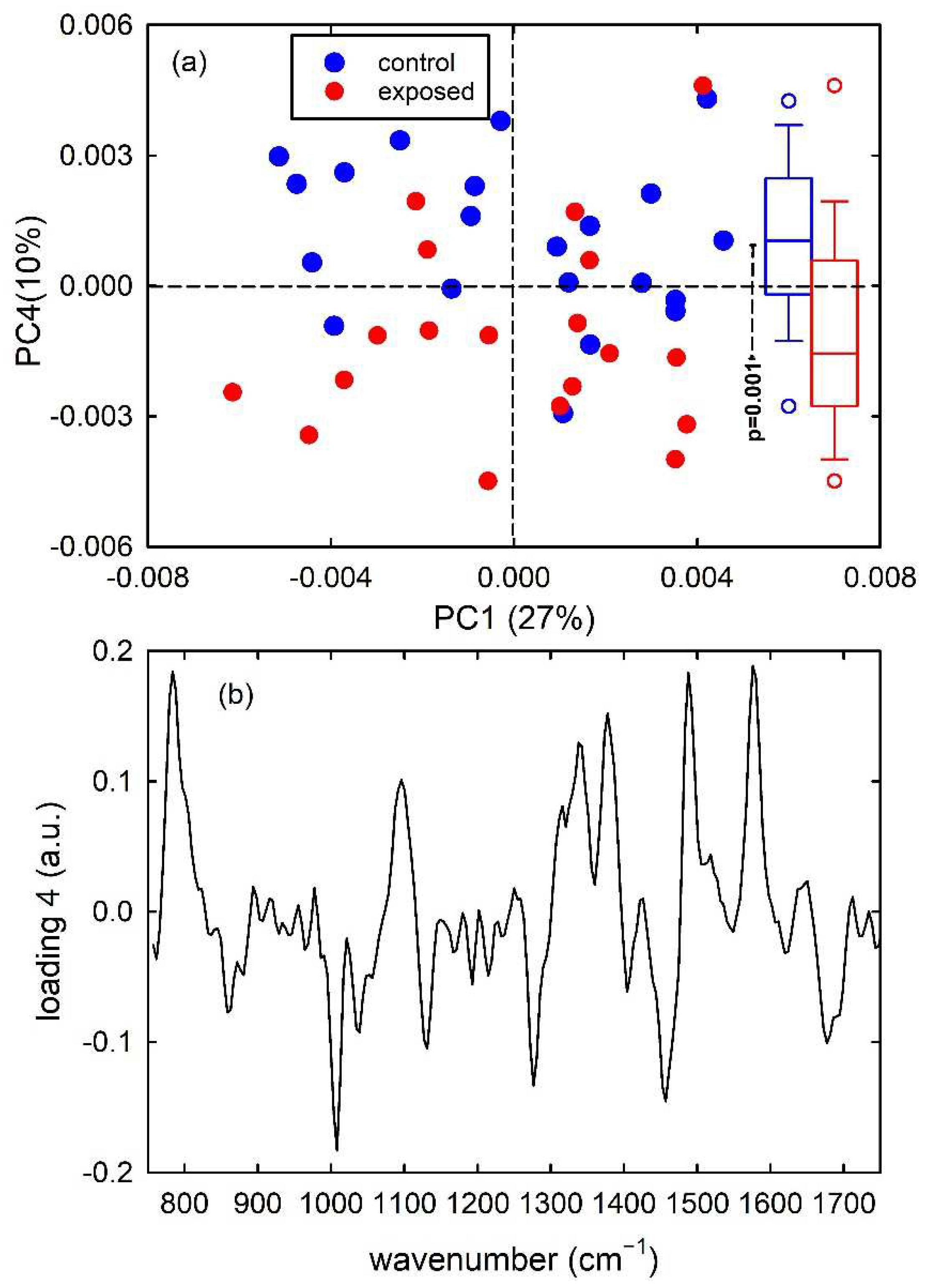
Similar results occur for Raman spectra of control- and proton-exposed MCF10A cells. For the spectra of such cells, the first 7 principal components carried around 90% of all the spectral variation found in the whole dataset. The score plot in Figure 5a points out that the PC4 component discriminates control from exposed cells, where control cells present mainly positive PC4 score values and exposed cells have mainly negative PC4 score values. Although overlapping score values are more major than in Figure 4a, the distributions of score values are statistically different, as can be deduced from the box plots on the right side of Figure 5a obtained by the t-test analysis. A confirmation that PC4 discriminates between the two types of cells is obtained from Figure 5b, where values of PC4 loadings are shown. The similarity of the spectrum in Figure 5b with that in Figure 2c is very evident. The positive peaks in Figure 5b correspond to Raman peaks due to nucleic acid cellular components, while the spectral positions of the negative peaks correspond to spectral Raman signals related to cellular protein and lipid components, as discussed above.
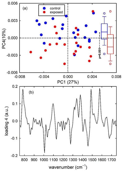
Figure 5.
PC4 vs. PC1 score plot (a) for the control (blue dots) and exposed (red dots) Raman spectra of MCF10A cells. The box plots of the PC4 score values are shown on the right side of (a): the results of the t-test point out that the two distributions of score values are significantly different (p = 0.001). Loading 4 spectrum is reported in (b).
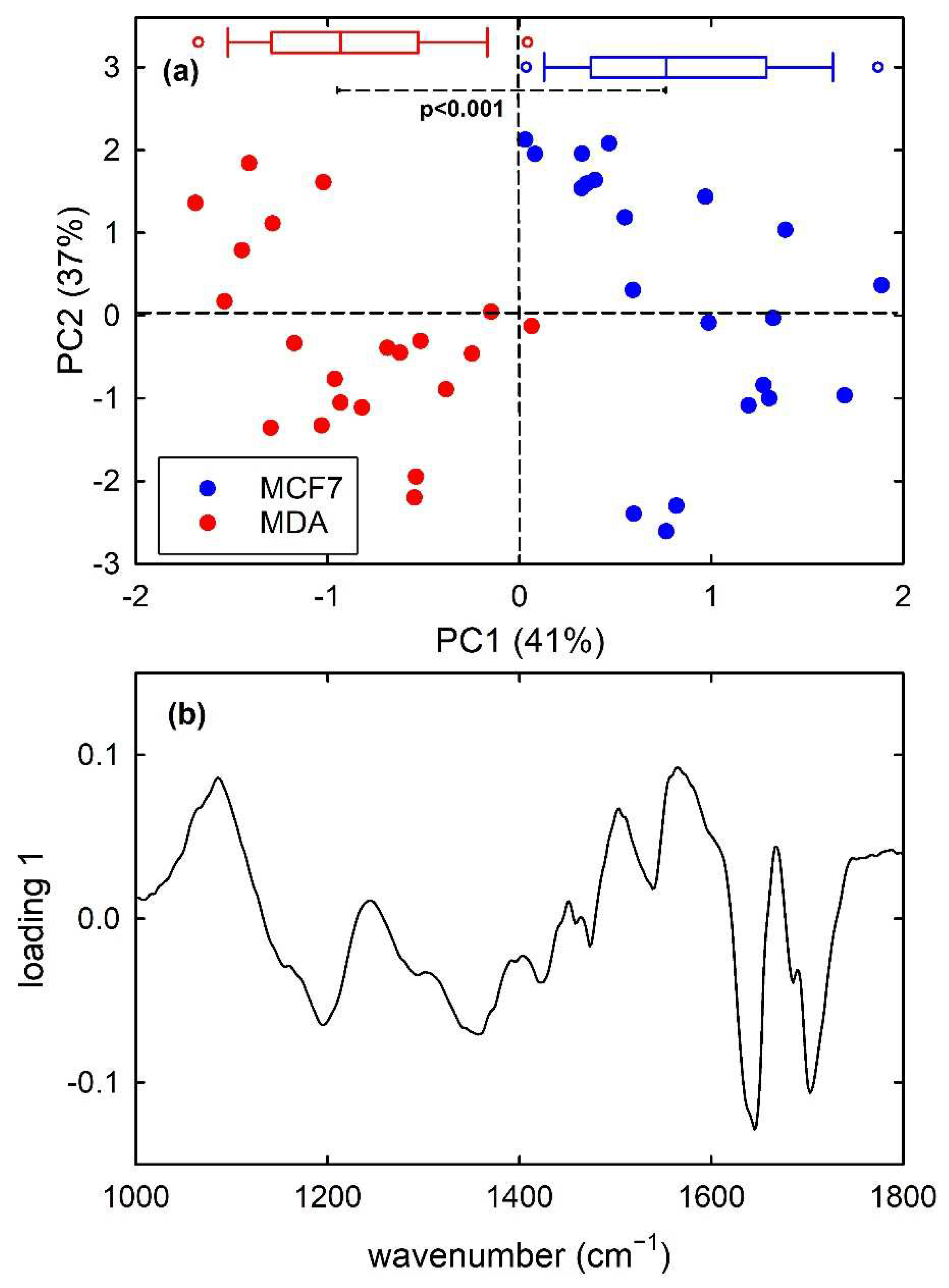
Finally, PCA results for the dataset of MCF7 and MDA cells are shown in Figure 6. For the FTIR spectra of this dataset, the first 7 principal components carried around 97% of all the spectral variation found in the whole dataset. The score plot in Figure 6a highlights that PC1 well discriminate the metastatic MDA cells from the malignant MCF7 ones, with almost no overlapping score values. In particular, MCF7 and MDA cells have positive and negative, respectively, PC1 score values and the box plots at the top of Figure 6a demonstrates that the two distribution are statistically different, according to t-test analysis. Furthermore, the loading 1 plot in Figure 6b is very similar to the difference plot in Figure 3c, indicating that MCF7 cells (positive score) have a large relative content of nucleic acid components (positive loading bands at about 1085 and 1230 cm−1) with respect to MDA cells, whereas the spectral features in the 1500–1700 cm−1 range are related to the shift of the spectral position of amide I and II bands for the two types of cell.
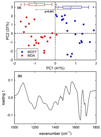
Figure 6.
PC2 vs. PC1 score plot (a) for the MCF7 (blue dots) and MDA (red dots) FTIR spectra. The box plots of the PC1 score values are shown at the top of (a): the results of the t-test point out that the two distributions of score values are significantly different (p < 0.001). Loading 1 spectrum is reported in (b).
Overall, the presence of several peaks in the loading plots of the discriminating PCs and the agreement of their spectral positions with those of the difference plots confirmed the discrimination potential of vibrational spectra. Therefore, classification techniques can be applied to the test sets of the three datasets, in order to evaluate the discrimination performance.
Hence, following the PCA, linear discrimination analysis was first performed. The first seven PC scores of the calibration set of simulated spectra were used as input data for LDA to build a diagnostic model that will be used for the classification of unknown spectra. The PCA-LDA model correctly classifies all the 36 spectra, as visible in the classification plot shown in Figure 7a (filled circles). In fact, a discriminant score for the attribution of an object (spectrum) to each class is calculated and the object is assigned to that class for which the discriminant score is the largest. Hence, in Figure 7a samples lying close to zero for a class are associated with that class. Instead, the accuracy of the PCA-LDA model for the classification of Raman spectra from unexposed and proton-exposed MCF10A cells, shown in Figure 7b is 87.5%. Indeed, such a model, obtained by using the first seven PC scores of the calibration set as input for the LDA model, erroneously attributes some samples of the calibration set to a different class from the one they actually belong to, as visible in Figure 7b from the circle crossed samples. In particular, 4 control spectra were attributed to exposed class and 1 exposed spectrum was attributed to control class. Lastly, a 100% accuracy is obtained for the PCA-LDA classification model related to MCF7 and MDA cells, as visible in Figure 7c.
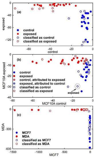
Figure 7.
Discrimination plot obtained from the results of Linear Discriminant Analysis model developed using 7 principal components from Principal Component Analysis. The scatter plot shows the discrimination of synthetic control-like spectra (filled blue circles) and exposed-like vibrational spectra (filled red circles) in (a), that of Raman spectra of control (filled blue circles) and exposed (filled red circles) MCF10A cells in (b) and that of FTIR spectra of MCF7 (filled blue circles) and MDA (filled red circles) cells in (c). Crossed circles in (b) are related to samples of the calibration set which are erroneously attributed to the PCA-LDA model. The projections of the test samples on the PCA-LDA model are shown as hollow circles. One misclassified sample of the test set is enclosed inside a circle and labelled in (b).
Despite the small number of spectra used by us, the accuracy value of the PCA-LDA model is similar to that obtained by T. Ning et al. regarding the discrimination of two different types of breast cancer tissue from healthy breast tissue by means of Raman spectroscopy: in fact, their accuracy, validated through full cross-validation, is equal to 88.3% [34]. Furthermore, Y. Lin et al. declared to discriminate breast cancer by SERS spectra of serum proteins from cancer patients with respect to those from healthy volunteers with the PCA-LDA model, achieving an accuracy value of 84% with a ten-fold cross-validation method [35]. Similar accuracy values with the PCA-LDA algorithm applied to Raman spectra have been obtained for discrimination of normal parenchyma and follicular patterned thyroid nodules (78%) and for carcinoma versus adenoma follicular lesions (89%) [36]. Furthermore, Raman spectra from normal and tumour oral tissues were differentiated under the PCA-LDA model with an accuracy of 81.25% with full and k-fold cross-validation methods [37].
Instead of cross-validation, we prefer to estimate the sensitivity and specificity of the classification model using a set of data (test set) that are external and independent of those used to build the model. This procedure is performed in view of its possible use in a clinical setting for diagnostic purposes. Indeed, in this case, some spectra should be acquired from areas containing material (cells, tissues) that are difficult to diagnose and the classification technique applied to these spectra, having available a dataset of spectra previously acquired from pathological and healthy areas.
Therefore, the prediction parameters of the developed PCA-LDA model were tested using samples of the test sets from the two classes. The results of the model prediction are summarized in Table 1. Almost all the tested samples were predicted as belonging to the proper class, except one MCF10A exposed sample which is attributed to the control class. Therefore, the model was able to rightly classify the test samples and the accuracy, sensitivity and specificity achieved maximum values in the cases of simulated spectra and FTIR spectra, whereas these values were 93%, 86% and 100%, respectively, in the case of proton-exposed MCF10A cells. In order to obtain a visual picture of the classification performance, the test samples were projected on the classification plot in Figure 7, where they are represented by hollow circles. It is clearly visible that all the representative points of the test set samples are in proximity to the representative points of the calibration set samples, with only one exception in Figure 7b due to an MCF10A exposed sample which has been misclassified, as discussed above.

Table 1.
Performance parameters for the three types of spectra. The parameter values are estimated by considering the results obtained for the spectra of the test sets. Accuracy represents the total rate of spectra correctly classified; sensitivity is the rate of spectra classified as exposed-like (for simulated spectra), exposed (for Raman spectra) and metastatic MDA (for FTIR spectra) with respect to the spectra which refer actually to exposed-like, exposed and MDA samples, respectively; specificity is the rate of spectra classified as control-like (for simulated spectra), control (for Raman spectra) and non-metastatic MCF7 (for FTIR spectra) with respect to the spectra which refer actually to control-like, control and MCF7 samples, respectively.
The procedure of optimizing the model using a calibration test with cross-validation and then evaluating the model performance using a test set was also carried out by H. Li et al., who measured Raman spectra from various types of breast cancer [38]. In particular, they found that the PCA-LDA model correctly classifies all samples in the test set. Furthermore, N. Iturrioz-Rodríguez et al. have recently used Raman spectroscopy and PCA-LDA model for the classification of glioblastoma multiforme cells derived from brain tumour patients versus astrocytes derived from healthy patients, using a test set consisting of different cells than the calibration set [18]. They stated an average classification accuracy of 92.5%. Therefore, the results we obtained about the performance parameters of the PCA-LDA technique applied to different types of vibrational spectra are in good agreement with those reported by other authors about spectra obtained with the Raman technique.
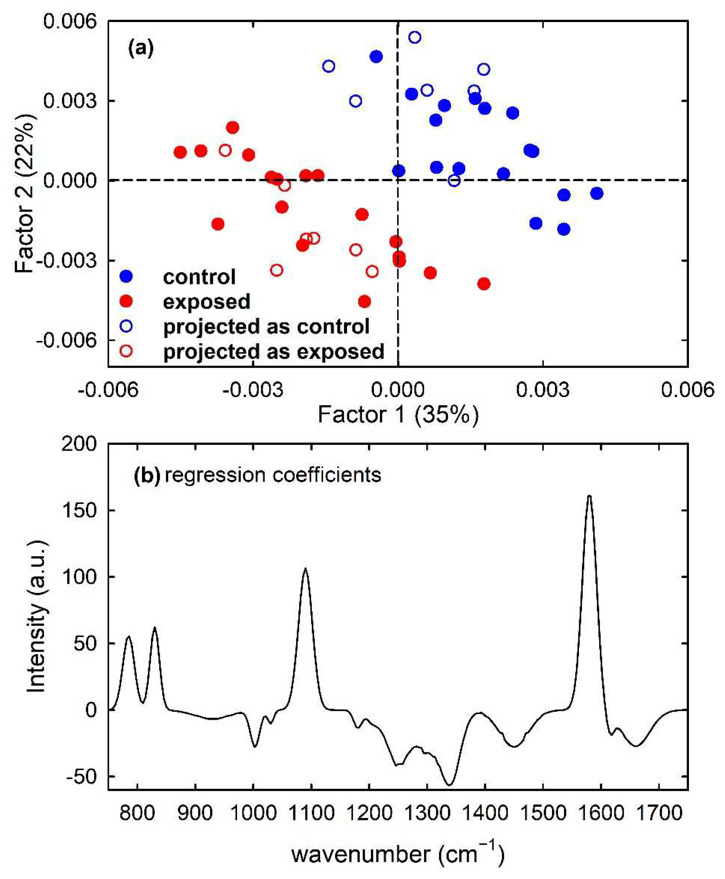
Furthermore, a PLS model was built for the calibration set of simulated spectra by using 7 latent variables. Clear discrimination of the control and exposed spectra is visible in Figure 8a, which shows (filled circles) the score plot of Factor 1 and Factor 2 of the PLS model. In particular, the separation between the two types of spectra can be observed along both factors. Such a feature is also confirmed by the plot of the regression coefficients, shown in Figure 8b for two components of the regression model. It can be deduced that the most important variables in the PLS model were those corresponding to wavenumbers around 780, 830, 1090 and 1580 cm−1, as expected because the spectral peaks centred at such wavenumber values are mainly responsible for the difference between the average spectra of control-like and exposed-like spectra reported in Figure 1c. The performance of the prediction ability of the built PLS model, checked by using just the samples from the test set, is summarized in Table 1. All the unknown samples were correctly assigned to the proper class, so producing maximum values of the performance parameters. Such results can be also visualized by reporting the projections of the test samples on the Factor 2 vs. Factor 1 score plot, shown as hollow circles in Figure 8a.
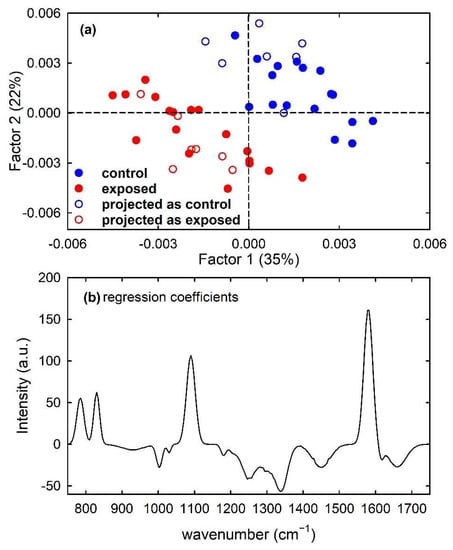
Figure 8.
Scores plot (Factor 2 vs. Factor 1) of the developed PLS-DA model, showing the calibration (filled circles) and projected test set (hollow circles) samples for the control-like (blue circles) and exposed-like (red circles) spectra in (a). The root mean square error for cross-validation (RMSECV) is 0.40. Regression coefficients for the PLS model with two components in (b).
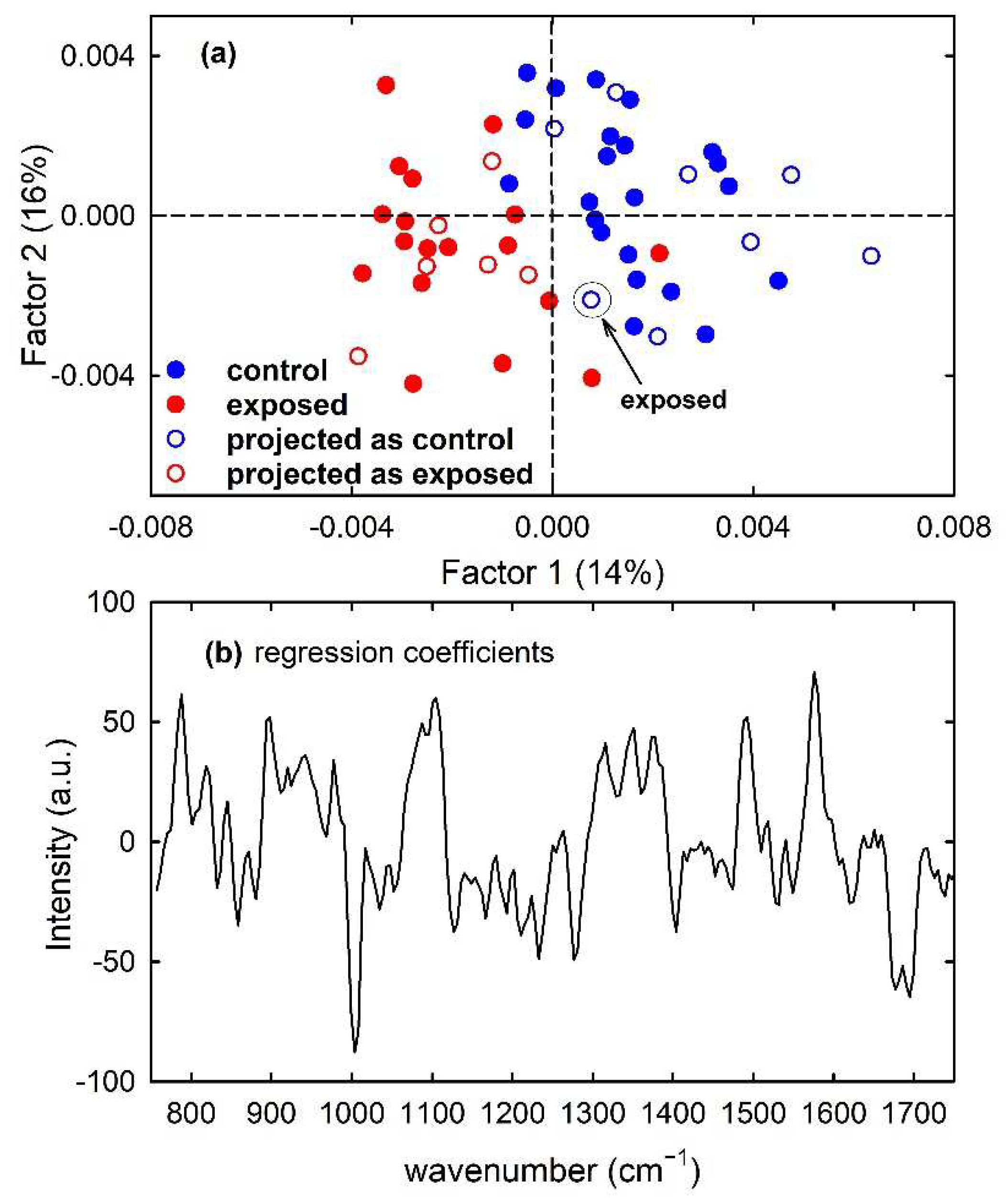
Similarly, the PLS model built for calibration samples of the MCF10A cells clearly discriminates control from exposed cells mainly according to Factor 1, as visible in Figure 9a with the filled circles. The similarity of the plot of regression coefficients with two components in Figure 9b with the difference between mean spectra of Figure 2c suggests that two factors are also able to correctly discriminate control from exposed samples according to the intensity of Raman peaks related to nucleic acids components. As for the prediction ability of the model, one exposed sample of the test set was misclassified, so determining accuracy and sensitivity values of 93% and 86%, respectively, as reported in Table 1 and visible in the scatter plot of the projected samples, shown as hollow circles in Figure 9a. The misclassified sample of the test set has been labelled for clarity.
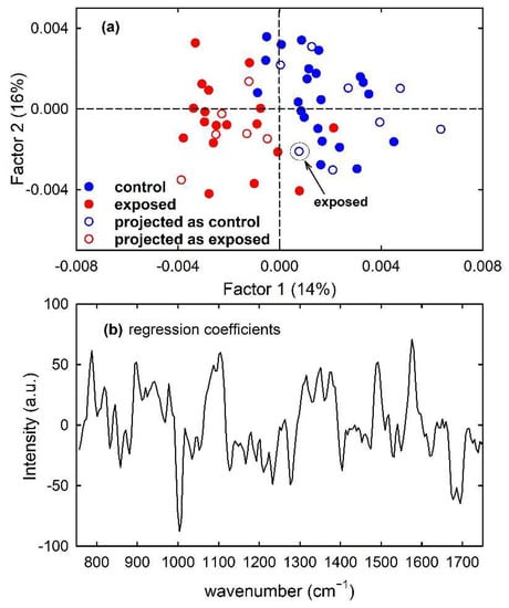
Figure 9.
Scores plot (Factor 2 vs. Factor 1) of the developed PLS-DA model about Raman spectra for control (blue circles) and exposed (red circles) MCF10A cells, showing the calibration (filled circles) and projected test set (hollow circles) samples in (a). The root mean square error for cross-validation (RMSECV) is 0.75. One misclassified sample of the test set is enclosed inside a circle and labelled in (a). Regression coefficients for the PLS model with two components in (b).
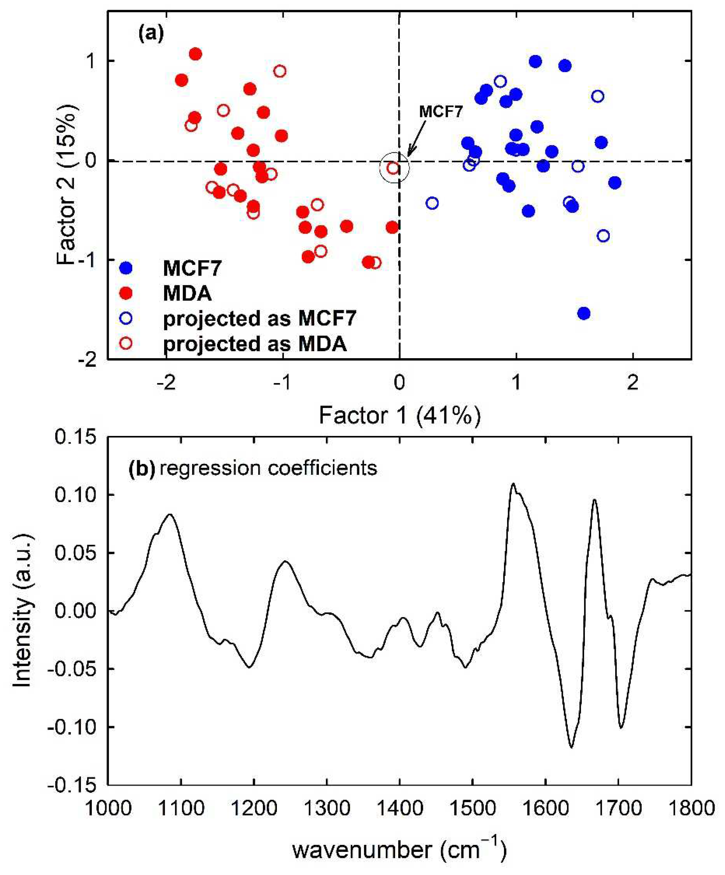
Furthermore, the PLS model developed from the calibration samples of the MCF7 and MDA cells rightly discriminates metastatic from malignant cells according to Factor 1, as visible in Figure 10a with the filled circles. The regression coefficients of the PLS model with two components are plotted in Figure 10b: the spectral shape of such plot is analogous to that of Figure 3c, which reports the difference spectrum between MCF7 and MDA mean spectra. Therefore, it can be deduced that two LVs correctly discriminate metastatic cells from malignant ones. Furthermore, in this case, the prediction ability of the model was good but not perfect because one MCF7 sample of the test set was misclassified, as reported in Table 1. The obtained sensitivity value was 100%, whereas the accuracy and specificity values were 95% and 90%, respectively. The misclassified sample is also visible in Figure 10a as red hollow circles which have been labelled for clarification purposes. In a comparison of the results obtained by the PLS-DA classification with those of the PCA-LDA classification, it is evident that the latter has a better performance in terms of accuracy and specificity.
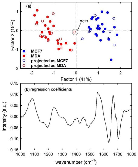
Figure 10.
Scores plot (Factor 2 vs. Factor 1) of the developed PLS-DA model about FTIR spectra for MCF7 (blue circles) and MDA (red circles) cells, showing the calibration (filled circles) and projected test set (hollow circles) samples in (a). The root mean square error for cross-validation (RMSECV) is 0.31. One misclassified sample of the test set is enclosed inside a circle and labelled in (a). Regression coefficients for the PLS model with two components in (b).
The above performance parameters values are better than those obtained by W. Liu et al., who used patient tissues measured by Raman spectroscopy associated with the PLS-DA model and full cross-validation to diagnose colorectal cancer with a sensitivity of 77.7%, a specificity of 91.0%, and an accuracy of 84.3% [39]. Surface-enhanced Raman spectroscopy combined with the Lasso-PLS-DA algorithm with full cross-validation was used by G. Chen et al. for the identification of different tumour states in nasopharyngeal cancer [40]: they yielded a diagnostic sensitivity of 68% and a specificity of 84.0% for separating T2-T4 stage from T1 stage cancer. Larger values of classification parameters were achieved by X. Yang et al., who declared 87.10% accuracy, 80% sensitivity and 91.89% specificity by using the PLS-DA model with test set validation to discriminate first derivative FTIR data in nucleic acids spectral range collected from serum samples of patients with lung cancer and healthy people [25]. Recently, high sensitivity and specificity values (more than 90%) were also reported for the discrimination of FTIR spectra measured for two different melanoma cell lines (primary IPC-298 and metastatic SK-MEL-30) by using the PLS-DA model with test set validation [41].
As evident from the above discussion, the PCA-LDA and PLS-DA techniques are widely used for the analysis and classification of spectral measurements, together with other multivariate data classification techniques [37,39,42,43,44]. However, they have been mainly used for single datasets including spectra of different types to obtain classifications (e.g., discrimination of spectra from healthy and diseased cells). On the contrary, in the present study, the two classification techniques were both used on three different types of very different spectral datasets, in order to obtain a comparison of the predictions, as independent as possible from the single dataset. This comparison is useful for choosing the optimal method. The comparison pointed out the good performance of both methods, with a prevalence of PCA-LDA which is able to classify FTIR spectra with better accuracy and specificity than PLS-DA.
4. Conclusions
In this study, both simulated and experimental vibrational spectra were used to investigate the ability of PCA-LDA and PLS-DA to discriminate spectra related to different classes. This investigation was carried out in two successive phases: firstly, classification algorithms were built with the two techniques, using a subset of each dataset as a calibration set; then, the performance of the constructed models was evaluated by analysing the classifications performed for a test set, obtained as subsets of the original datasets but which did not include any of the spectra used for the calibration set. The obtained results were evaluated according to the values of accuracy, sensitivity and specificity in the classification of the spectra of the test set of the three datasets. They showed that both models have good performance, although the PCA-LDA model seems a little better than the PLS-DA model for a lightly major accuracy and specificity in the classification of FTIR spectra.
Although good results have been achieved in the classification of vibrational spectra, our study has been designed as a “proof of concept”, because it presents limits that must be overcome before a possible adoption of multivariate classification of vibrational spectra for diagnostic purposes could be envisaged. The main limit to overcome concerns the small number of spectra included in our datasets. In fact, this number would have to be increased considerably in order to obtain ever more reliable values of the classification parameters. So, our achieved results should be considered preliminary data. In addition, our results were obtained for simulated spectra as well as for cell-lines-measured spectra. They should be confirmed by using ex vivo cells extracted from biopsies of patients, as well as by using tissues and biofluids. Eventually, it is also necessary to evaluate the performances of other classification techniques (e.g., k-nearest neighbours, soft independent modelling of class analogies, support-vector machine,...) in order to evaluate whether they are able to classify unknown spectra even better than the PCA-LDA and PLS-DA. Nonetheless, the proposed approach is promising, especially if a PCA-LDA or a PLS model has been built with a dataset of spectra from samples whose pathological state is known (healthy, disease, at different stages of the disease, etc.). In this case, a few tens of spectra from the unknown sample should be measured and considered as test sets for which to perform the classification by PCA-LDA or PLS-DA and, consequently, make the diagnosis.
Supplementary Materials
The following supporting information can be downloaded at: https://www.mdpi.com/article/10.3390/app12115345/s1, Table S1: Values of spectral parameters amplitude (Ai), wavenumber (x0i) and broadening (σi) for each Gaussian peak of the basic control-like and exposed-like vibrational spectrum.
Author Contributions
Formal analysis, G.P.; Investigation, M.L.; Supervision, V.C.; Writing—original draft, M.L. and G.P. All authors have read and agreed to the published version of the manuscript.
Funding
This research received no external funding.
Institutional Review Board Statement
Not applicable.
Informed Consent Statement
Not applicable.
Data Availability Statement
Not applicable.
Conflicts of Interest
The authors declare no conflict of interest.
References
- Traynor, D.; Behl, I.; O’Dea, D.; Bonnier, F.; Nicholson, S.; O’Connell, F.; Maguire, A.; Flint, S.; Galvin, S.; Healy, C.M.; et al. Raman spectral cytopathology for cancer diagnostic applications. Nat. Protoc. 2021, 16, 3716–3735. [Google Scholar] [CrossRef] [PubMed]
- Severcan, F.; Haris, P.I. Vibrational Spectroscopy in Diagnosis and Screening; IOS Press: Amsterdam, The Netherlands, 2012. [Google Scholar]
- Sbroscia, M.; Di Gioacchino, M.; Ascenzi, P.; Crucitti, P.; Di Masi, A.; Giovannoni, I.; Longo, F.; Mariotti, D.; Naciu, A.M.; Palermo, A.; et al. Thyroid cancer diagnosis by Raman spectroscopy. Sci. Rep. 2020, 10, 13342. [Google Scholar] [CrossRef] [PubMed]
- Bangaoil, R.; Santillan, A.; Angeles, L.M.; Abanilla, L.; Lim, A., Jr.; Ramos, M.C.; Fellizar, A.; Guevarra, L., Jr.; Albano, P.M. ATR-FTIR spectroscopy as adjunct method to the microscopic examination of hematoxylin and eosin-stained tissues in diagnosing lung cancer. PLoS ONE 2020, 15, e0233626. [Google Scholar]
- Beć, K.B.; Grabska, J.; Huck, C.W. Biomolecular and bioanalytical applications of infrared spectroscopy—A review. Anal. Chim. Acta 2020, 1133, 150–177. [Google Scholar] [CrossRef]
- Byrne, H.J.; Behl, I.; Calado, G.; Ibrahim, O.; Toner, M.; Galvin, S.; Healy, C.M.; Flint, S.; Lyng, F.M. Biomedical applications of vibrational spectroscopy: Oral cancer diagnostics. Acta Part A Mol. Biomol. Spectrosc. 2021, 252, 119470. [Google Scholar] [CrossRef]
- McCreery, R.L. Raman Spectroscopy for Chemical Analysis; Winefordner, J.D., Ed.; Wiley & Sons: New York, NY, USA, 2000. [Google Scholar]
- Griffiths, P.R.; de Haseth, J.A. Fourier Transform Infrared Spectrometry; Winefordner, J.D., Ed.; Wiley & Sons: New York, NY, USA, 2007. [Google Scholar]
- Gautam, R.; Vanga, S.; Ariese, F.; Umapathy, S. Review of multidimensional data processing approaches for Raman and infrared spectroscopy. EPJ Tech. Instrum. 2015, 2, 8. [Google Scholar] [CrossRef] [Green Version]
- Morais, C.L.M.; Lima, K.M.G.; Singh, M.; Martin, F.L. Tutorial: Multivariate classification for vibrational spectroscopy in biological samples. Nat. Protoc. 2020, 15, 2143–2162. [Google Scholar] [CrossRef]
- Varmuza, K.; Filzmoser, P. Introduction to Multivariate Statistical Analysis in Chemometrics; CRC Press: Boca Raton, FL, USA, 2009. [Google Scholar]
- Jolliffe, I.T.; Cadima, J. Principal component analysis: A review and recent developments. Philos. Trans. R. Soc. A Math. Phys. Eng. Sci. 2016, 374, 20150202. [Google Scholar] [CrossRef]
- Knief, P.; Keating, M.E.; Bonnier, F.; Byrne, H.J. Spectral pre and post processing for infrared and Raman spectroscopy of biological tissues and cells. Chem. Soc. Rev. 2016, 45, 1865–1878. [Google Scholar]
- Bonnier, F.; Byrne, H.J. Understanding the molecular information contained in principal component analysis of vibrational spectra of biological systems. Analyst 2012, 137, 322–332. [Google Scholar] [CrossRef] [Green Version]
- Lim, J.-Y.; Nam, J.-S.; Shin, H.; Park, J.; Song, H.-I.; Kang, M.; Lim, K.-I.; Choi, Y. Identification of Newly Emerging Influenza Viruses by Detecting the Virally Infected Cells Based on Surface Enhanced Raman Spectroscopy and Principal Component Analysis. Anal. Chem. 2019, 91, 5677–5684. [Google Scholar] [CrossRef]
- Ong, Y.H.; Lim, M.; Liu, Q. Comparison of principal component analysis and biochemical component analysis in Raman spectroscopy for the discrimination of apoptosis and necrosis in K562 leukemia cells. Opt. Express 2012, 20, 22158–22171. [Google Scholar] [CrossRef]
- Morais, C.L.M.; Paraskevaidi, M.; Cui, L.; Fullwood, N.J.; Isabelle, M.; Lima, K.M.G.; Martin-Hirsch, P.L.; Sreedhar, H.; Trevisan, J.; Walsh, M.J.; et al. Standardization of complex biologically derived spectrochemical datasets. Nat. Protoc. 2019, 14, 1546–1577. [Google Scholar] [CrossRef] [Green Version]
- Iturrioz-Rodríguez, N.; De Pasquale, D.; Fiaschi, P.; Ciofani, G. Discrimination of glioma patient-derived cells from healthy astrocytes by exploiting Raman spectroscopy. Spectrochim. Acta Part A Mol. Biomol. Spectrosc. 2022, 269, 120773. [Google Scholar] [CrossRef]
- Falamas, A.; Faur, C.I.; Ciupe, S.; Chirila, M.; Rotaru, H.; Hedesiu, M.; Pinzaru, S.C. Rapid and noninvasive diagnosis of oral and oropharyngeal cancer based on micro-Raman and FT-IR spectra of saliva. Spectrochim. Acta Part A Mol. Biomol. Spectrosc. 2021, 252, 119477. [Google Scholar] [CrossRef]
- Ali, S.; Naseer, K.; Qazi, J. Diagnosis of HCV infection using attenuated total Reflection-FTIR spectra of Freeze-Dried sera. Infrared Phys. Technol. 2022, 121, 104019. [Google Scholar] [CrossRef]
- Malonek, D.; Dekel, B.; Haran, G.; Reens-Carmel, R.; Groisman, G.M.; Hallak, M.; Bruchim, I. Rapid intraoperative diagnosis of gynecological cancer by ATR-FTIR spectroscopy of fresh tissue biopsy. J. Biophotonics 2020, 13, e202000114. [Google Scholar] [CrossRef]
- Lee, L.C.; Liong, C.Y.; Jemain, A.A. Partial least squares-discriminant analysis (PLS-DA) for classification of high-dimensional (HD) data: A review of contemporary practice strategies and knowledge gaps. Analyst 2018, 143, 3526–3539. [Google Scholar] [CrossRef]
- Aguiar, R.P.; Falcão, E.T.; Pasqualucci, C.A.; Silveira, L. Use of Raman spectroscopy to evaluate the biochemical composition of normal and tumoral human brain tissues for diagnosis. Lasers Med. Sci. 2020, 37, 121–133. [Google Scholar] [CrossRef]
- Cullen, D.; Bryant, J.; Maguire, A.; Medipally, D.; McClean, B.; Shields, L.; Noone, E.; Bradshaw, S.; Finn, M.; Dunne, M.; et al. Raman spectroscopy of lymphocytes for the identification of prostate cancer patients with late radiation toxicity following radiotherapy. Transl. Biophotonics 2020, 2, e201900035. [Google Scholar] [CrossRef]
- Yang, X.; Ou, Q.; Qian, K.; Yang, J.; Bai, Z.; Yang, W.; Shi, Y.; Liu, G. Diagnosis of Lung Cancer by ATR-FTIR Spectroscopy and Chemometrics. Front. Oncol. 2021, 11, 753791. [Google Scholar] [CrossRef]
- Ildiz, G.O.; Karadag, A.; Kaygisiz, E.; Fausto, R. PLS-DA Model for the Evaluation of Attention Deficit and Hyperactivity Disorder in Children and Adolescents through Blood Serum FTIR Spectra. Molecules 2021, 26, 3400. [Google Scholar] [CrossRef]
- Lasalvia, M.; Perna, G.; Pisciotta, P.; Cammarata, F.P.; Manti, L.; Capozzi, V. Raman spectroscopy for the evaluation of the radiobiological sensitivity of normal human breast cells at different time points after irradiation by a clinical proton beam. Analyst 2019, 144, 2097–2108. [Google Scholar] [CrossRef]
- Lasalvia, M.; Capozzi, V.; Perna, G. Comparison of FTIR spectra of different breast cell lines to detect spectral biomarkers of pathology. Infrared Phys. Technol. 2022, 120, 103976. [Google Scholar] [CrossRef]
- Talari, A.C.S.; Movasaghi, Z.; Rehman, S.; ur Rehman, I. Raman Spectroscopy of Biological Tissues. Appl. Spectrosc. Rev. 2015, 50, 46–111. [Google Scholar] [CrossRef]
- Synytsya, A.; Alexa, P.; de Boer, J.; Loewe, M.; Moosburger, M.; Wurkner, M.; Volka, K. Raman spectroscopic study of calf thymus DNA: An effect of proton- and γ-irradiation. J. Raman Spectrosc. 2007, 38, 1406–1415. [Google Scholar] [CrossRef]
- Sofińska, K.; Wilkosz, N.; Szymoński, M.; Lipiec, E. Molecular Spectroscopic Markers of DNA Damage. Molecules 2020, 25, 561. [Google Scholar] [CrossRef] [Green Version]
- Talari, A.C.S.; Evans, C.A.; Holen, I.; Coleman, R.E.; Rehman, I.U. Raman spectroscopic analysis differentiates between breast cancer cell lines. J. Raman Spectrosc. 2015, 46, 421–427. [Google Scholar] [CrossRef]
- Abramczyk, H.; Surmacki, J.; Kope’c, M.; Olejnik, A.K.; Lubecka-Pietruszewska, K.; Fabianowska-Majewska, K. The role of lipid droplets and adipocytes in cancer. Raman imaging of cell cultures: MCF10A, MCF7, and MDA-MB-231 compared to adipocytes in cancerous human breast tissue. Analyst 2015, 140, 2224–2235. [Google Scholar] [CrossRef]
- Ning, T.; Li, H.; Chen, Y.; Zhang, B.; Zhang, F.; Wang, S. Raman spectroscopy based pathological analysis and discrimination of formalin fixed paraffin embedded breast cancer tissue. Vib. Spectrosc. 2021, 115, 103260. [Google Scholar] [CrossRef]
- Lin, Y.; Gao, J.; Tang, S.; Zhao, X.; Zheng, M.; Gong, W.; Xie, S.; Gao, S.; Yu, Y.; Lin, J. Label-free diagnosis of breast cancer based on serum protein purification assisted surface-enhanced Raman spectroscopy. Spectrochim. Acta Part A Mol. Biomol. Spectrosc. 2021, 263, 120234. [Google Scholar] [CrossRef] [PubMed]
- Rau, J.V.; Fosca, M.; Graziani, V.; Taffon, C.; Rocchia, M.; Caricato, M.; Pozzilli, P.; Muda, A.O.; Crescenzi, A. Proof-of-concept Raman spectroscopy study aimedto differentiate thyroid follicular patterned lesions. Sci. Rep. 2017, 7, 14970. [Google Scholar] [CrossRef] [PubMed] [Green Version]
- Jeng, M.J.; Sharma, M.; Sharma, L.; Chao, T.Y.; Huang, S.F.; Chang, L.B.; Wu, S.L.; Chow, L. Raman Spectroscopy Analysis for Optical Diagnosis of Oral Cancer Detection. J. Clin. Med. 2019, 8, 1313. [Google Scholar] [CrossRef] [PubMed]
- Li, H.; Ning, T.; Yu, F.; Chen, Y.; Zhang, B.; Wang, S. Raman Microspectroscopic Investigation and Classification of Breast Cancer Pathological Characteristics. Molecules 2021, 26, 921. [Google Scholar] [CrossRef] [PubMed]
- Liu, W.; Sun, Z.; Chen, J.; Jing, C. Raman Spectroscopy in Colorectal Cancer Diagnostics: Comparison of PCA-LDA and PLS-DA Models. J. Spectrosc. 2016, 2016, 1603609. [Google Scholar] [CrossRef]
- Chen, G.; Lin, X.; Lin, D.; Ge, X.; Feng, S. Identification of different tumor states in nasopharyngeal cancer using surface-enhanced Raman spectroscopy combined with Lasso-PLS-DA algorithm. RSC Adv. 2016, 6, 7760–7764. [Google Scholar] [CrossRef]
- Shakya, B.R.; Teppo, H.R.; Rieppo, L. Optimization of measurement mode and sample processing for FTIR microspectroscopy in skin cancer research. Analyst 2022, 147, 851–861. [Google Scholar] [CrossRef]
- Lilo, T.; Morais, C.L.M.; Ashton, K.M.; Pardilho, A.; Davis, C.; Dawson, T.P.; Gurusinghe, N.; Martin, F.L. Spectrochemical differentiation of meningioma tumours based on attenuated total reflection Fourier-transform infrared (ATR-FTIR) spectroscopy. Anal. Bioanal. Chem. 2020, 412, 1077–1086. [Google Scholar] [CrossRef] [Green Version]
- Chatchawal, P.; Wongwattanakul, M.; Tippayawat, P.; Kochan, K.; Jearanaikoon, N.; Wood, B.R.; Jearanaikoon, P. Detection of Human Cholangiocarcinoma Markers in Serum Using Infrared Spectroscopy. Cancers 2021, 13, 5109. [Google Scholar] [CrossRef]
- Goulart, A.C.C.; Silveira, L., Jr.; Carvalho, H.C.; Dorta, C.B.; Pacheco, M.T.T.; Zângaro, R.A. Diagnosing COVID-19 in human serum using Raman spectroscopy. Lasers Med. Sci. 2022, 14, 1–10. [Google Scholar] [CrossRef]
Publisher’s Note: MDPI stays neutral with regard to jurisdictional claims in published maps and institutional affiliations. |
© 2022 by the authors. Licensee MDPI, Basel, Switzerland. This article is an open access article distributed under the terms and conditions of the Creative Commons Attribution (CC BY) license (https://creativecommons.org/licenses/by/4.0/).

