On the Sum of α-μ/Inverse Gamma Variates with Applications to Diversity Receivers

Abstract

How to model shadow fading by applying the inverse gamma (IGA) distribution has recently gained widespread attention in wireless transmissions. However, the sum of α-μ/IGA variates, and its applications under independent and/or correlated scenarios, have yet to be addressed in open research works. Hence, this paper provides a systematic investigation of the α-μ/IGA model. First, we derive the expressions of the fundamental statistics of the univariate and bivariate α-μ/IGA models including the probability density function, cumulative distribution function, and moment generating function, and propose a mixture α-μ model to approximate the α-μ/IGA model. Then, according to the above statistical expressions, the statistical properties of the sum of α-μ/IGA variates are obtained and employed in the maximal ratio combining receivers. Third, the novel exact and approximated expressions of some performance metrics of interest are also derived, for instance, the average bit/symbol error probability, the outage probability, the average channel capacity, and the effective rate. Moreover, to prove the asymptotic properties of the performance metrics at the high signal-to-noise regions, some examples are performed. Finally, we explore numerical analysis and simulations to demonstrate the accuracy of the theoretical expressions under the different channel and system parameters. These results provide some significant insights into the reliability design and deployment of some conventional and emerging wireless communication applications.

1. Introduction

In the past decades, how to model wireless fading channels accurately has been an important and inevitable topic in the research of conventional and emerging wireless communication systems, such as cellular networks, wearable communications, and vehicular wireless networks. Generally, the received signals of wireless transmission undergo either small-scale (multipath) fading or large-scale (shadowing) fading, or even the composite effects of both. For small-scale fading, some classical fading models have been reported in [1], namely the Rayleigh, the Rice, the Nakagami-m, the Weibull, and so on. To accurately characterize the envelope fluctuation of the received signals and better fit empirical data encountered in some emerging wireless applications, some more general and sophisticated versions of the above multipath fading models have also been proposed, such as η-μ, κ-μ, α-μ, α-η-μ, α-κ-μ and α-η-κ-μ in [2] and references therein. For large-scale fading, the lognormal (LN) model is a typical shadowing fading example [1]. Unfortunately, the main disadvantage of this model is that its probability density function (PDF) contains an integral form which limits its applications for performance analysis purposes. For this reason, two substituted versions of the LN model have been proposed to approximate it, namely the Gamma (GA) model [3] and the inverse Gaussian (IG) model [4]. However, in some practical wireless communication scenarios, the composite effects of both multipath and shadowing fading become a dominating fading phenomenon. To this end, the composite fading models have been extensively explored by combining multipath fading with shadowing, which comprise the LN-based composite model (such as Rayleigh/LN, Rice/LN, Nakagami/LN, Weibull/LN, α-η-μ/LN, and α-κ-μ/LN [5]), the GA-based composite model (such as Rayleigh/GA, Nakagami/GA, Weibull/GA, η-μ/GA, κ-μ/GA, and α-μ/GA [6]), the IG-based model (such as Rayleigh/IG, Nakagami/IG, η-μ/IG, κ-μ/IG, and α-μ/IG [7]), the line-of-sight (LOS) shadowing composite model (such as Rician shadowed [1] and κ-μ shadowed [8]), and the double shadowing composite model [9,10]. Furthermore, a double α-μ model in [11,12] has also been proposed to describe the composite multipath-shadowing models, where the first α-μ model denotes the multipath fading and the second one is the shadowing fading.

More recently, an inverse Gamma (IGA) model to characterize shadowing has been widely studied to achieve an appropriate balance between modeling accuracy and calculation complexity. For the empirical field measurements of the IGA model, the authors in [13] provided the experimental studies through wearable communication channels tests to prove that the underlying IGA model shadowing is very available compared with the LN and the GA models. At the same time, the authors in [14,15] also confirmed that describing light and moderate shadowing with the IGA model is a reasonable alternative for the LN and the GA models by considering more testing scenarios, including both indoor and outdoor with many different frequency bands. More importantly, [14,15] showed some mathematical expressions based on the IGA model are more tractable and simpler than those by using the LN or the IG model. By employing the IGA shadowing model, an unmanned aerial vehicle-to-ground communications channel model was presented in [16] which can provide a notable fit for empirical data.

For the application of the underlying IGA model, [17,18] first obtained the average symbol error rate of multiple amplitude modulation and the ergodic capacity over κ-μ/IGA and η-μ/IGA composite fading channels, respectively. After that, the same authors pointed out in [19] that the κ-μ/IGA and η-μ/IGA models not only provide a good fit for modeling the composite fading channels but also can be extended to the conventional and emerging wireless communication systems, such as cellular, wearable, and vehicular wireless applications. However, they only derived the statistical characteristics of the η-μ/IGA and κ-μ/IGA models, which include the PDF, the cumulative distribution function (CDF), the moment generating function (MGF), the higher-order moments, and the amount of fading. In [20], the effective capacity was analyzed over η-μ/IGA and κ-μ/IGA composite fading channels. In [21], the average symbol error probability (ASEP) and the channel capacity with adaptive schemes were obtained over η-μ/IGA and κ-μ/IGA composite fading channels. Moreover, some performance analysis was investigated over the inverse gamma pure shadowed fading channels in [22,23]. As a counterpart of η-μ/IGA and κ-μ/IGA, the α-μ/IGA composite model has also been involved in [24,25,26], where [24] obtained the performance analysis of the single-branch system with the aid of Fox’H functions, [25] developed the energy detection of single-branch and maximal-ratio combining (MRC) systems over independent and identical distributed (i.i.d.) conditions, and [26] provided an approximated performance analysis of MRC and equal gain combining (EGC) by using a mixed IGA distribution under i.i.d. conditions. In recent work, the authors in [27] presented the α-η-μ/IGA and α-κ-μ/IGA channel models and evaluated the performance of multi-hop links.

On the other hand, the Fisher-Snedecor $\mathcal{F}$ fading channel model in [28] can be considered as an alternative version of the IGA-based composite model based upon the fact that the square root of an IGA random variable (RV) follows an inverse Nakagami-m distribution. So far, this model has obtained extensive interest and a great number of works have been done in [29,30,31] and references therein. By considering the nonlinearity of the composite envelope of fading signals, the α-$\mathcal{F}$, the α-η-$\mathcal{F}$, the α-κ-$\mathcal{F}$, and α-η-κ-$\mathcal{F}$ composite fading models were presented in [32,33,34], respectively. When α = 2, these three models can reduce to the Fisher-Snedecor $\mathcal{F}$, the η-μ/IGA, and κ-μ/IGA, respectively. Although the α-η-μ/IGA, α-κ-μ/IGA, the α-η-$\mathcal{F}$, the α-κ-$\mathcal{F}$, and α-η-κ-$\mathcal{F}$ are versatile, the mathematical forms of their PDFs are still intractable, which renders them rather difficult to analyze the performance of wireless communication systems exactly.

Based on the above observation, most of the works involving the IGA shadowing model focused on the Fisher-Snedecor $\mathcal{F}$, the η-μ/IGA, and κ-μ/IGA fading channels. Although the α-μ/IGA model has been considered in [24,25,26], to the best of the authors’ knowledge, a comprehensive investigation of wireless communication systems over α-μ/IGA composite fading channels has not yet been involved in the independent and non-identical distributed (i.n.i.d.) scenarios and/or the correlated scenarios. To this effect, we will further extend our work in [24] to provide a thorough investigation and some significant insights into the α-μ/IGA and its application in wireless communication systems. In addition, this model can also be potentially applied to describe the distribution of population densities and urban activities investigated in [35]. In this paper, we first drive the exact analytical formulations of the statistical characteristics of univariate and bivariate α-μ/IGA distributions and compare the differences between the α-μ/IGA and the α-$\mathcal{F}$ models, as well as a new mixture α-μ model and the mixture IGA model. Then, capitalizing on the obtained statistical expressions, the PDF, the CDF, and the MGF of the sum of α-μ/IGA variates are derived in the i.n.i.d. and the correlated scenarios in the light of the multivariate Fox’s H-function by utilizing the Mellin-Barnes type contour integral, respectively. At the same time, some exact approximated expressions are also deduced by using the mixture α-μ model. Thirdly, some performance metrics of interest for the single-link and MRC systems are investigated, respectively, including the outage probability (OP), the average bit/symbol error probability (ABEP/ASEP), and the average channel capacity and the effective rate. In addition, the asymptotic analysis of the ABEP of DPSK (Differential Phase Shift Keying) and the OP are considered at high signal-to-noise (SNR) regions. Finally, the numerical analysis and simulations are carried out to confirm the accuracy of our theoretical derivations in various scenarios.

The remainder of this paper is organized as follows: In Section 2, the statistical features of the univariate and bivariate α-μ/IGA distributions are investigated, and some comparisons are discussed. Some exact and approximated analytical expressions of the statistical properties of the sum of α-μ/IGA variates are obtained in Section 3. Section 4 derives the analytical expressions of performance metrics including the OP, the ABEP/ASEP, the channel capacity, and the effective capacity. In Section 5, we show some asymptotic analysis by using several examples in high SNR regions. Then, the numerical evaluations and simulations are performed and discussed in Section 6. Finally, we conclude the whole paper in Section 7.

2. Statistical Characteristics of α-μ/IGA Distribution

2.1. Univariate Case

In the α-μ/IGA composite fading environments, the amplitude of the multipath envelopes of the α-μ distribution suffers from random fluctuations induced by an IGA shadowing RV. Thus, the received signal envelope R can be expressed as

$$R^2=Z{R}_{\alpha -u}^{\alpha }={\displaystyle \sum _{i=1}^{\mu }Z(X_i^2+Y_i^2)},$$

(1)

where $R_{\alpha -\mu }$ denotes the envelope of α-μ distribution, Z follows the IGA distribution, α is the non-linear parameter and α > 0, μ represents the number of multipath clusters, and $\mu$ $\ge 1/2$, $X_i$, and $Y_i$ are mutually independent Gaussian RVs with zero-mean and average power ${\sigma }^2$, which represent the in-phase and quadrature components of cluster i. Hence, the PDF of R can be obtained by averaging the conditional PDF of the α-μ fading process over the statistics of the IGA shadowing RV. Mathematically,

$$f_R(r)={\displaystyle {\int }_0^{\infty }{f}_{R|Z}(r|z)f_Z(z)dz},$$

(2)

where $f_{R|Z}(r|z)$ is the conditional PDF of the α-μ fading distribution in [36] with respect to RV z, as follows

$$f_{R|Z}(r|z)=\frac{\alpha {\beta }^{0.5\alpha \mu }{r}^{\alpha \mu -1}}{\mathsf{\Gamma }(\mu ){(z\mathsf{\Omega })}^{0.5\alpha \mu }}\exp [-\frac{{\beta }^{0.5\alpha }{r}^{\alpha }}{{(z\mathsf{\Omega })}^{0.5\alpha }}],$$

(3)

where $\mathbb{E}\left[r^2\right]=\mathsf{\Omega }$, $\beta$ $=\mathsf{\Gamma }\left(\mu +\raisebox{1ex}{$2$}\!\left/ \!\raisebox{-1ex}{$\alpha $}\right.\right)/\mathsf{\Gamma }\left(\mu \right)$ represents the power scale factor, $\mathbb{E}[\cdot ]$denoting the statistical mean, and $\mathsf{\Gamma }(·)$ is the gamma function defined in ([37], Equation (8.310.1)). In (2), $f_Z\left(z\right)$ is the PDF of the IGA distribution to model shadowing fading in [15], and can be given by

$$f_Z(z)=\frac{{(n-1)}^n}{\mathsf{\Gamma }(n)}{z}^{-(n+1)}\exp (-\frac{n-1}{z}),$$

(4)

where n denotes the shape parameter and $n>1$, $\mathbb{E}\left[\mathrm{z}\right]=1$. Note that $n\to 1$ denotes the received signals are subject to the heavy shadowing; on the contrary, $n\to \infty$ represents the absence of shadowing. Substituting (3) and (4) in (2), the PDF of the received signal envelope R can be expressed as

$$f_R(r)=\frac{\alpha {\beta }^{0.5\alpha \mu }{(n-1)}^n{r}^{\alpha \mu -1}}{\mathsf{\Gamma }(\mu )\mathsf{\Gamma }(n){\mathsf{\Omega }}^{0.5\alpha \mu }}{\displaystyle {\int }_0^{\infty }{z}^{-(n+0.5\alpha \mu +1)}\exp (-\frac{n-1}{z})\exp [-\frac{{\beta }^{0.5\alpha }{r}^{\alpha }}{{(z\mathsf{\Omega })}^{0.5\alpha }}]dy}.$$

(5)

To obtain the closed-form expression of the PDF of the composite envelope R, we represent the exponential form $\exp \left(-x\right)$ in terms of Fox’s H function ${\mathrm{H}}_{0,1}^{1,0}\left[x{|}_{\left(0,1\right)}^{-}\right]$by using the identity ([38], Equation (1.125)). After a simple variable transformation and based on the definition of Fox’s H function in [38] (Equation (1.2)), (5) can be rewritten as

$$f_R(r)=\frac{\alpha r^{-1}}{\mathsf{\Gamma }(\mu )\mathsf{\Gamma }(n)}{H}_{1,1}^{1,1}[\frac{{\beta }^{0.5\alpha }{r}^{\alpha }}{{[(n-1)\mathsf{\Omega }]}^{0.5\alpha }}|{}_{(\mu ,1)}^{(1-n,0.5\alpha )}],$$

(6)

where $H_{p,q}^{m,n}[·|·]$ denotes a univariate Fox’s H-function. Similar to the η-μ/IGA and κ-μ/IGA models, the α-μ/IGA composite distribution is also a generalized composite distribution. As α = 2, this model is equivalent to the Fisher-Snedecor $\mathcal{F}$ composite fading model proposed in [28]. As μ = 1, the α-μ/IGA distribution reduces to Weibull/IGA. By setting α = 2 and μ = 1, this model results in Rayleigh/IGA, whilst $n\to \infty$, the α-μ model becomes its special case. Here, we let the instantaneous SNR $\gamma =r^2{E}_s/N_0$, where $E_s$ is the average energy per symbol and $N_0$ denotes the single-sided power spectral density, then the average SNR can be given as $\overline{\gamma }=\mathsf{\Omega }{E}_s/N_0$. Thus, by using (6) and applying the change of variables, the corresponding PDF of $\gamma$ can be obtained as

$$f_{\gamma }(\gamma )=\frac{\alpha {\gamma }^{-1}}{2\mathsf{\Gamma }(\mu )\mathsf{\Gamma }(n)}{H}_{1,1}^{1,1}[\lambda {\gamma }^{0.5\alpha }|{}_{(\mu ,1)}^{(1-n,0.5\alpha )}],$$

(7)

where $\lambda ={(\beta /\left(n-1\right)\overline{\gamma })}^{0.5\alpha }$. Obviously, (7) can reduce to [39] (Equation (2)) as α = 2 by using the identity [38] (Equation (1.60)). Invoking the definition of the univariate Fox’s H-function and using the similar derived process of (6), the corresponding CDF and MGF of $\gamma$ can be obtained, respectively, as

$$F_{\gamma }(\gamma )={\displaystyle {\int }_0^{\gamma }{f}_{\gamma }(\gamma )d\gamma }=\frac{1}{\mathsf{\Gamma }(\mu )\mathsf{\Gamma }(n)}{H}_{2,2}^{1,2}[\lambda {\gamma }^{0.5\alpha }|{}_{(\mu ,1),(0,1)}^{(1-n,0.5\alpha ),(1,1)}],$$

(8)

$$MG{F}_{\gamma }(s)={\displaystyle {\int }_0^{\infty }\exp (-s\gamma )f_{\gamma }(\gamma )d\gamma }=\frac{\alpha }{2\mathsf{\Gamma }(\mu )\mathsf{\Gamma }(n)}{H}_{2,1}^{1,2}[\lambda s^{-0.5\alpha }|{}_{(\mu ,1)}^{(1-n,0.5\alpha ),(1,0.5\alpha )}].$$

(9)

It is noted here that (8) and (9) can also reduce to [40] (Equation (2)), [41] (Equation (2)) as α = 2, respectively. Interestingly, the Fisher-Snedecor $\mathcal{F}$ model is also a special case of the α-$\mathcal{F}$ distribution. In [32], the α-$\mathcal{F}$ model was deduced from the $\mathcal{F}$ model by using a power transformation, and its signal envelope R is expressed as $R^{\alpha }={\displaystyle \sum }_{i=1}^{\mu }Z\left(X_i^2+Y_i^2\right)$. From the right-hand side of (1), the α-μ/IGA and α-$\mathcal{F}$ models have the identical mathematical form and physical parameters including α, μ, and n. However, they have different physical interpretations from the view of the physical processes of the signal envelopes. The former represents the mean of the non-linear multipath envelopes is subject to the shadowing effects following the IGA distribution, whereas the latter can be considered as the composite envelopes following the $\mathcal{F}$ distribution encounter the non-linear propagation in a nonhomogeneous environment.

For the sake of comparison, we evaluated the impacts of the physical parameters on the PDFs of both models in Figure 1. It can be observed from Figure 1 that as α = 2, both models reduce to the $\mathcal{F}$ one, while as α ≠ 2 and n = 5 (moderate shadowing), they diverge greatly from each other. With the increase in the value of shadowing parameters (n = 5→50), they tend to have similar results, which indicates the shadowing effects decrease, and they reduce to the α-μ model. Moreover, the parameter μ shows the same effect on the PDFs of both models when μ grows. This is because the nonlinear feature of the α-$\mathcal{F}$ model affects both μ and n, while only μ is affected by its nonlinear parameter in the α-μ/IGA model. As expected, the PDF curves of both models converge to around the average SNR ($\overline{\gamma }=1$) when the values of α and μ get larger, which means good channel conditions.

Recently, several mixed PDF models were presented to provide some accurate approximated expressions via the Gaussian-Laguerre quadrature approximation and overcome certain mathematical difficulties, such as the mixture Gamma (MG) distribution [41] and the mixture inverse Gaussian distribution [7]. By applying similar approaches, the exact closed-form expression of (6) can also be approximated as a mixed form of the IGA or the α-μ distribution. In [26], the mixture IGA model has been considered to approximate the α-μ/IGA model just as the MG distribution was used to approximate the α-μ/GA model in [6]. However, it was reported in [26] that the number of the truncation term is large and goes up to 45 in order to achieve the error <10⁻⁵. To this end, we consider an alternative new form to approximate the α-μ/IGA model. By letting $t=\left(n-1\right)/z$ in (5) and performing some straightforward manipulations and several the changes of variables, (7) can be approximated as

$$f_{\gamma }(\gamma )={\displaystyle \sum _{i=1}^N{\varsigma }_i\frac{\alpha {\gamma }^{0.5\alpha \mu -1}}{2\mathsf{\Gamma }(\mu ){\psi }_i^{0.5\alpha \mu }}\exp [-\frac{{\gamma }^{0.5\alpha }}{{\psi }_i{}^{0.5\alpha }}]},$$

(10)

where ${\varsigma }_i={\omega }_i{t}_i^{\mu -1}/\mathsf{\Gamma }\left(n\right)$, ${\psi }_i=\overline{\gamma }\left(n-1\right)/(\beta t_i)$, N denotes the number of truncation terms, and ${\omega }_i$ and $t_i$ are the abscissas and weight factors for the Gaussian-Laguerre integration, respectively. Here, we name the novel form in (10) as a mixed α-μ distribution model. In particular, this model is a generalized version of the MG distribution and can be referred to as the generalized MG (GMG) distribution. Most noteworthy is that the α-X multipath and α-μ-Y composited fading distributions can be simplified as this mixture sum form, where X denotes η-μ or κ-μ, and Y denotes LN, Gamma, or α-μ [11] distribution models.

Based on the definition in (8) and (9), and using (10), the corresponding approximated forms of the CDF and the MGF of $\gamma$ can be obtained, respectively, as

$$F_{\gamma }(\gamma )={\displaystyle \sum _{i=1}^N\frac{{\varsigma }_i\gamma (\mu ,{(\gamma /{\psi }_i)}^{0.5\alpha })}{\mathsf{\Gamma }(\mu )}},$$

(11)

$$MG{F}_{\gamma }(s)={\displaystyle \sum _{i=1}^N\frac{{\varsigma }_i\alpha }{2\mathsf{\Gamma }(\mu )}{H}_{1,1}^{1,1}[{(s{\psi }_i)}^{-0.5\alpha }|{}_{(\mu ,1)}^{(1,0.5\alpha )}]},$$

(12)

where $\gamma \left(·,·\right)$ is the lower incomplete gamma function defined in [37] (Equation (8.310.1)). In order to prove the accuracy of the approximated distribution models, two classical criteria of error are often adopted to evaluate the error between the exact PDF and the approximated PDF in [41], namely the mean square error (MSE) and the Kullback-Leibler divergence (KLD). For the purposes of comparison, the approximated PDF of$\gamma$ based on the mixed IGA model can be expressed as [26]

$$f_{\gamma }(\gamma )={\displaystyle \sum _{i=1}^N\frac{{\xi }_i{\eta }_i^n}{\mathsf{\Gamma }(n)}{\gamma }^{-n-1}\exp [-{\eta }_i{\gamma }^{-1}]},$$

(13)

where ${\xi }_i={\omega }_i{t}_i^{\mu -1}/\mathsf{\Gamma }\left(\mu \right)$, ${\eta }_i=\overline{\gamma }\left(n-1\right){\left(t_i/\beta \right)}^{2/\alpha }$.

In Figure 2a–d, we compare the exact PDF in (7), the mixed α-μ PDF in (10), and the mixed IGA PDF in (13) under different conditions, and present the impacts of various parameters on the PDFs. At the same time, the Monte Carlo simulations are also provided to validate the accuracy of the approximated distributions. From Figure 2a–d, it can be observed that the PDF curves of the mixed IGA model show the larger divergences when the values of the truncated terms (N), α, and/or μ are smaller (for example, N = 8, 12 in Figure 2a, α = 1.5 in Figure 2b, and μ = 1.5 in Figure 2d), or the values of the shadowing parameter, n, become larger (for example, n = 20 in Figure 2c), whereas it is interesting that the PDF curves of the mixed α-μ achieve good agreements with the exact PDF in (7) in most of the cases except the case where α = 5 and N = 8 in Figure 2b. Although increasing the value of N can reduce the divergences between the exact PDF and the mixed IGA, it renders more computation complexity and a longer running time. Furthermore, with the aid of the definitions of MSE and KLD in [42], the error analytical results are calculated under various fading scenarios in

Table 1. Comparisons of the MSE and the KLD for the exact PDF and the mixed PDFs with different channel parameters (α, μ, and n) and the truncated term (N).

Channel Parameters		N = 8				N = 20
		Mixed IGA		Mixed α-μ		Mixed IGA		Mixed α-μ
		MSE	KLD	MSE	KLD	MSE	KLD	MSE	KLD
α = 2, μ = 2	n = 2	0.001158	0.007285	1.148 × 10−5	0.009336	9.947 × 10−5	0.001056	3.008 × 10−8	6.149 × 10−4
	n = 20	0.03936	0.4076	2.766 × 10−5	0.009583	0.008485	0.09145	2.933 × 10−19	1.816 × 10−9
α = 2, n = 5	μ = 1	0.05102	1.5389	4.759 × 10−11	2.399 × 10−5	0.02487	0.5276	9.694 × 10−20	8.243 × 10−10
	μ = 5	1.491 × 10−5	2.3875 × 10−4	1.258 × 10−6	4.8473 × 10−4	1.886 × 10−8	3.608 × 10−6	1.047 × 10−10	1.048 × 10−5
α = 2, n = 5	α = 1	0.1449	0.3154	2.345 × 10−12	5.906 × 10−6	0.03569	0.08006	2.536 × 10−17	2.433 × 10−8
	α = 5	2.526 × 10−5	8.651 × 10−4	2.366 × 10−4	0.007668	1.012 × 10−6	1.378 × 10−4	8.094 × 10−7	4.4059 × 10−4

. From Table 1, we can also obtain the same conclusions as ones from Figure 2a–d. Despite the mixed α-μ distribution being used to simplify the α-κ-μ shadowed model in [43], its fading parameters (μ and m) are constrained to be positive integers and cannot be extended to other models, as well as having no application for it. To the best of the authors’ knowledge, the mixed α-μ PDF in (10) is novel and has not yet been reported in the open technical papers. Based on the above results, the mixed α-μ distribution will be discussed in the following sections.

2.2. Bivariate Case

In the performance evaluations of wireless digital communication systems, the bivariate distributions are often used to analyze the performance of diversity receivers over correlated fading environments, such as [1,29]. So far, the bivariate α-μ/IGA composited distribution has not been considered in the previous works. In this context, we will derive the analytical expressions of the statistical properties of the bivariate α-μ/IGA distribution.

Let R_i (i = 1, 2) represent the channel fading envelope of α-μ processes, then, the joint conditional PDF between R₁ and R₂ can be expressed from [36] (Equation (28)) as

$$\begin{array}{cc}{f}_{R_1|W_1,R_2|W_2}(r_1|w_1,r_2|w_1)\hfill & =\frac{{\alpha }_1{\alpha }_2{r}_1^{0.5{\alpha }_1(\mu +1)-1}{r}_2^{0.5{\alpha }_2(\mu +1)-1}{\rho }_N^{-(\mu -1)/2}}{\mathsf{\Gamma }(\mu ){(\sqrt{{({\beta }_1/w_1{\mathsf{\Omega }}_1)}^{0.5{\alpha }_1}{({\beta }_2/w_2{\mathsf{\Omega }}_2)}^{0.5{\alpha }_2}})}^{(\mu +1)}(1-{\rho }_N)}\hfill \\ & \times \exp \left[-\frac{1}{1-{\rho }_N}\left(\frac{r_1^{{\alpha }_1}{\beta }_1^{0.5{\alpha }_1}}{{(w_1{\mathsf{\Omega }}_1)}^{0.5{\alpha }_1}}+\frac{r_2^{{\alpha }_2}{\beta }_2^{0.5{\alpha }_2}}{{(w_2{\mathsf{\Omega }}_2)}^{0.5{\alpha }_2}}\right)\right]I_{\mu -1}\left[\frac{2}{(1-{\rho }_N)}\sqrt{\frac{{\rho }_N{r}_1^{{\alpha }_1}{r}_2^{{\alpha }_2}{\beta }_1^{0.5{\alpha }_1}{\beta }_2^{0.5{\alpha }_2}}{{(w_1{\mathsf{\Omega }}_1)}^{0.5{\alpha }_1}{(w_2{\mathsf{\Omega }}_2)}^{0.5{\alpha }_2}}}\right],\end{array}$$

(14)

where ${\alpha }_i$ is the nonlinear fading parameter, ${\rho }_N$ is the power correlation coefficient between $R_1^2$ and $R_2^2$, and $I_{\mu -1}\left(x\right)$ represents the modified Bessel function of the first kind and order (μ − 1) defined in [36] (Equation (9.210/1)), ${\beta }_i=\mathsf{\Gamma }\left(\mathsf{\mu }+2/{\alpha }_i\right)/\mathsf{\Gamma }\left(\mu \right)$. When multipath fading is superimposed on shadowing, $W_i$ slowly varies. Here, we assume $W_i$ follows the IGA distribution in (4) and $\mathbb{E}\left[r_i^2\right]={\mathsf{\Omega }}_i$. By using a simple operation of Equation (8) given in [44], the joint PDF of the bivariate IGA distribution can be derived as

$$f_{W_1,W_2}(w_1,w_2)=\frac{{(n-1)}^{n+1}{(w_1{w}_2)}^{-0.5(n+3)}}{\mathsf{\Gamma }(n)(1-{\rho }_G){\rho }_G^{(n-1)/2}}\exp \left[-\frac{(n-1)(w_1^{-1}+w_2^{-1})}{1-{\rho }_G}\right]I_{n-1}\left[\frac{2(n-1)\sqrt{{\rho }_G}}{\sqrt{w_1{w}_2}(1-{\rho }_G)}\right],$$

(15)

where $n>1$is the IGA shaping parameter, ${\rho }_G$ is the power correlation coefficient between $w_1^2$ and $w_2^2$, and $\mathbb{E}\left[w_i\right]$ = 1.

Thus, by using the same approach shown in [29] (Equation (5)), and performing some basic operations, the joint PDF of the bivariate α-μ/IGA composite distribution is written as

$$f_{R_1,R_2}(r_1,r_2)={\displaystyle \sum _{k=0}^{\infty }{\displaystyle \sum _{l=0}^{\infty }\frac{\mathsf{\Phi }{\rho }_N^k{\rho }_G^l{r}_1^{-1}{r}_2^{-1}}{k!l!\mathsf{\Gamma }(k+\mu )\mathsf{\Gamma }(l+n)}{\displaystyle {\prod }_{i=1}^2{H}_{1,1}^{1,1}[{\mathsf{\Xi }}_i{r}_i^{{\alpha }_i}{|}_{(\mu +k,1)}^{(1-n-l,0.5{\alpha }_i)}]}}},$$

(16)

where $\mathsf{\Phi }={\alpha }_1{\alpha }_2{(1-{\rho }_G)}^n{(1-{\rho }_N)}^{\mu }/[\mathsf{\Gamma }(\mu )\mathsf{\Gamma }(n)]$, ${\mathsf{\Xi }}_i={((1-{\rho }_G){\beta }_i)}^{0.5{\alpha }_i}/[(1-{\rho }_N){({\mathsf{\Omega }}_i(n-1))}^{0.5{\alpha }_i}]$.

By setting ${\gamma }_i=r_i^2{E}_s/N_0$ and ${\overline{\gamma }}_i={\mathsf{\Omega }}_i{E}_s/N_0$, after a simple variable transformation, the joint PDF of ${\gamma }_1$ and ${\gamma }_2$ over the correlated α-μ/IGA channels can be obtained as

$$f_{{\gamma }_1,{\gamma }_2}({\gamma }_1,{\gamma }_2)={\displaystyle \sum _{k=0}^{\infty }{\displaystyle \sum _{l=0}^{\infty }\frac{0.25\mathsf{\Phi }{\rho }_N^k{\rho }_G^l{\gamma }_1^{-1}{\gamma }_2^{-1}}{k!l!\mathsf{\Gamma }(k+\mu )\mathsf{\Gamma }(l+n)}{\displaystyle {\prod }_{i=1}^2{H}_{1,1}^{1,1}[{\vartheta }_i{\gamma }_i^{0.5{\alpha }_i}{|}_{(\mu +k,1)}^{(1-n-l,0.5{\alpha }_i)}]}}},$$

(17)

where ${\vartheta }_i={((1-{\rho }_G){\beta }_i)}^{0.5{\alpha }_i}/[(1-{\rho }_N){((n-1){\overline{\gamma }}_i)}^{0.5{\alpha }_i}]$. Hence, with the aid of [37] (Equation (3.194.1)), the corresponding joint CDF of${\gamma }_1$ and ${\gamma }_2$ can be yielded as

$$\begin{array}{cc}{F}_{{\gamma }_1,{\gamma }_2}({\gamma }_1,{\gamma }_2)& ={\displaystyle {\int }_0^{{\gamma }_1}{\displaystyle {\int }_0^{{\gamma }_2}{f}_{{\gamma }_1,{\gamma }_2}({\gamma }_1,{\gamma }_2)d{\gamma }_{1}d{\gamma }_2}}\\ & ={\displaystyle \sum _{k=0}^{\infty }{\displaystyle \sum _{l=0}^{\infty }\frac{0.25\mathsf{\Phi }{\rho }_N^k{\rho }_G^l}{k!l!\mathsf{\Gamma }(k+\mu )\mathsf{\Gamma }(l+n)}{\displaystyle {\prod }_{i=1}^2{H}_{2,2}^{1,2}[{\vartheta }_i{\gamma }_i^{0.5{\alpha }_i}{|}_{(\mu +k,1),(0,0.5{\alpha }_i)}^{(1,0.5{\alpha }_i),(1-n-l,0.5{\alpha }_i)}]}}}.\end{array}$$

(18)

Moreover, based on the definition of the joint MGF in [1], the joint MGF of ${\gamma }_1$ and ${\gamma }_2$ can be given by

$$\begin{array}{cc}{M}_{{\gamma }_1,{\gamma }_2}(s_1,s_2)& =\mathbb{E}[\exp (-s_1{\gamma }_1-s_2{\gamma }_2)]\\ & ={\displaystyle \sum _{k=0}^{\infty }{\displaystyle \sum _{l=0}^{\infty }\frac{0.25\mathsf{\Phi }{\rho }_N^k{\rho }_G^l}{k!l!\mathsf{\Gamma }(k+\mu )\mathsf{\Gamma }(l+n)}{\displaystyle {\prod }_{i=1}^2{H}_{2,1}^{1,2}[{\vartheta }_i{s}_i^{-0.5{\alpha }_i}{|}_{(\mu +k,1)}^{(1,0.5{\alpha }_i),(1-n-l,0.5{\alpha }_i)}]}}}.\end{array}$$

(19)

3. Statistical Characteristics of the Sum of α-μ/IGA RVs

In this section, the statistical properties of the sum of L α-μ/IGA RVs are investigated. The classical application of the sum of RVs in diversity systems is to evaluate the performance of MRC and EGC systems, and only the MRC system is considered here. To this effect, we first derive the exact closed-form expressions of PDF, CDF, and MGF of the instantaneous output SNR for the MRC system in the i.n.i.d. case. Then, their corresponding approximated expressions are obtained based on the mixture α-μ model, respectively. Finally, their correlated statistics are acquired when L = 2.

3.1. Exact Statistics of the Sum of the Independent RVs

Let ${\gamma }_{MRC}={\displaystyle \sum }_{l=1}^L{\gamma }_l$, where ${\gamma }_l$ is the i.n.i.d. α-μ/IGA RV with the PDF in (7), the average SNR $\overline{{\gamma }_l}$, the fading parameters ${\alpha }_l$, ${\mu }_l$, and $n_l$, $l=1,\cdots ,L$, and L is the number of the RVs, then the PDF of ${\gamma }_{MRC}$ is yielded by

$$f_{{\gamma }_{MRC}}(\gamma )={\mathsf{\Theta }}_1{\gamma }^{-1}{H}_{0,1:{[2,1]}_{l=1:L}}^{0,0:{[1,2]}_{l=1:L}}[{\lambda }_1{\gamma }^{0.5{\alpha }_1},\cdots ,{\lambda }_L{\gamma }^{0.5{\alpha }_L}|{}_{(1;{\left\{0.5{\alpha }_l\right\}}_{l=1:L})}^{(-)}|{}_{{[({\mu }_l,1)]}_{{}_{l=1:L}}}^{{[(1-n_l,0.5{\alpha }_l),(1,0.5{\alpha }_l)]}_{{}_{l=1:L}}}],$$

(20)

where ${\mathsf{\Theta }}_1={\displaystyle \prod }_{l=1}^L{\alpha }_l/\left[2\mathsf{\Gamma }\left({\mu }_l\right)\mathsf{\Gamma }\left(n_l\right)\right]$,$H_{p,q:p_1,q_1:\cdots :p_L,q_L}^{m,n:m_1,n_1:\cdots :m_L,n_L}[·]$ denotes a multivariate Fox’s H-function defined in [38] (Equation (A.1)),${\lambda }_l={({\beta }_l/\left(n_l-1\right){\overline{\gamma }}_l)}^{0.5{\alpha }_l}$, ${\beta }_l=\mathsf{\Gamma }\left({\mu }_l+\raisebox{1ex}{$2$}\!\left/ \!\raisebox{-1ex}{${\alpha }_l$}\right.\right)/\mathsf{\Gamma }\left({\mu }_l\right)$.

Proof: Please refer to Appendix A.

Accordingly, based on the definition of the CDF and performing one definite integral of (20), the corresponding CDF of the sum of L α-μ/IGA RVs, ${\gamma }_{MRC}$, can be expressed as

$$F_{{\gamma }_{MRC}}(\gamma )={\mathsf{\Theta }}_1{H}_{0,1:{[2,1]}_{l=1:L}}^{0,0:{[1,2]}_{l=1:L}}[{\lambda }_1{\gamma }^{0.5{\alpha }_1},\cdots ,{\lambda }_L{\gamma }^{0.5{\alpha }_L}|{}_{(0;{\left\{0.5{\alpha }_l\right\}}_{l=1:L})}^{(-)}|{}_{{[({\mu }_l,1)]}_{{}_{l=1:L}}}^{{[(1-n_l,0.5{\alpha }_l),(1,0.5{\alpha }_l)]}_{{}_{l=1:L}}}].$$

(21)

For the i.i.d. case, (20) and (21) can be simplified by omitting the subscript.

3.2. Approximated Statistics of the Sum of the Independent RVs

By using (A1) and (12), the approximated MGF of ${\gamma }_{MRC}$ can be obtained as

$$MG{F}_{{\gamma }_{MRC}}(s)={\displaystyle \prod _{l=1}^{L}MG{F}_{{\gamma }_l}(s)}={\displaystyle \prod _{l=1}^L\left({\displaystyle \sum _{i_l=1}^{N_l}\frac{{\varsigma }_{i_l}{\alpha }_l}{2\mathsf{\Gamma }({\mu }_l)}{H}_{1,1}^{1,1}[{(s{\psi }_{i_l})}^{-0.5{\alpha }_l}|{}_{({\mu }_l,1)}^{(1,0.5{\alpha }_l)}]}\right)}.$$

(22)

For ease of calculation, we swap the order of the sum and the product in the right-hand side formula in (22); (22) can then be re-expressed in multiple summation forms as

$$MG{F}_{{\gamma }_{MRC}}(s)={\displaystyle \sum _{i_1=1}^{N_1}\cdots {\displaystyle \sum _{i_L=1}^{N_L}{\displaystyle \prod _{l=1}^L\left(\frac{{\varsigma }_{i_l}{\alpha }_l}{2\mathsf{\Gamma }({\mu }_l)}{H}_{1,1}^{1,1}[{(s{\psi }_{i_l})}^{-0.5{\alpha }_l}|{}_{({\mu }_l,1)}^{(1,0.5{\alpha }_l)}]\right)}}}$$

(23)

By utilizing (23) and the similar derivation procedure as Appendix A, the approximated PDF of ${\gamma }_{MRC}$ can be obtained as

$$f_{{\gamma }_{MRC}}(\gamma )={\displaystyle \sum _{i_1=1}^{N_1}\cdots {\displaystyle \sum _{i_L=1}^{N_L}\left[\left({\displaystyle \prod _{l=1}^L\frac{{\varsigma }_{i_l}{\alpha }_l}{2\mathsf{\Gamma }({\mu }_l)}}\right){\gamma }^{-1}{H}_{0,1:{[1,1]}_{l=1:L}}^{0,0:{[1,1]}_{l=1:L}}[{\left(\gamma /{\psi }_{i_1}\right)}^{0.5{\alpha }_1},\cdots ,{\left(\gamma /{\psi }_{i_L}\right)}^{0.5{\alpha }_L}|{}_{(1;{\left\{0.5{\alpha }_l\right\}}_{l=1:L})}^{-}|{}_{{[({\mu }_l,1)]}_{{}_{l=1:L}}}^{{[(1,0.5{\alpha }_l)]}_{{}_{l=1:L}}}]\right]}}.$$

(24)

From (21) and (24), we can see the summation forms in (24) bring the reduction of arguments in the multivariate Fox’s H-function. Importantly, (24) is a unified analytical expression and can be applied to more channel models where the PDF can be expressed as a mixture α-μ form in (10), such as α-η-μ and α-κ-μ, α-η-μ/lognormal and α-κ-μ/lognormal in [5], α-μ/gamma in [6], and α-μ/α-μ in [12]. Hence, the corresponding approximated CDF of ${\gamma }_{MRC}$ can be derived as

$$F_{{\gamma }_{MRC}}(\gamma )={\displaystyle \sum _{i_1=1}^{N_1}\cdots {\displaystyle \sum _{i_L=1}^{N_L}\left[\left({\displaystyle \prod _{l=1}^L\frac{{\varsigma }_{i_l}{\alpha }_l}{2\mathsf{\Gamma }({\mu }_l)}}\right)H_{0,1:{[1,1]}_{l=1:L}}^{0,0:{[1,1]}_{l=1:L}}[{\left(\gamma /{\psi }_{i_1}\right)}^{0.5{\alpha }_1},\cdots ,{\left(\gamma /{\psi }_{i_L}\right)}^{0.5{\alpha }_L}|{}_{(0;{\left\{0.5{\alpha }_l\right\}}_{l=1:L})}^{-}|{}_{{[({\mu }_l,1)]}_{{}_{l=1:L}}}^{{[(1,0.5{\alpha }_l)]}_{{}_{l=1:L}}}]\right]}}.$$

(25)

In the i.i.d. case, (22) can be simplified as

$$MG{F}_{{\gamma }_{MRC}}(s)={\left({\displaystyle \sum _{i=1}^N\frac{{\varsigma }_i\alpha }{2\mathsf{\Gamma }(\mu )}{H}_{1,1}^{1,1}[{(s{\psi }_i)}^{-0.5\alpha }|{}_{(\mu ,1)}^{(1,0.5\alpha )}]}\right)}^L$$

(26)

By applying the multinomial theorem, (26) can be rewritten as

$$MG{F}_{{\gamma }_{MRC}}(s)={\displaystyle \sum _{k_1+\cdots +k_N=L}\left(\begin{array}{c}L\\ k_1,\cdots ,k_N\end{array}\right)\underset{I_1}{\underbrace{{\displaystyle \prod _{1\le i\le N}{\left(\frac{{\varsigma }_i\alpha }{2\mathsf{\Gamma }(\mu )}{H}_{1,1}^{1,1}[{(s{\psi }_i)}^{-0.5\alpha }|{}_{(\mu ,1)}^{(1,0.5\alpha )}]\right)}^{k_i}} }}},$$

(27)

where ${\displaystyle \sum _{k_1+\cdots +k_N=L}}={\displaystyle \sum _{k_1=0}^L{\displaystyle \sum _{k_2=0}^{L-k_1}\cdots {\displaystyle \sum _{k_{N-1}=0}^{L-k_1-\cdots -k_{N-2}}}}}$, $\left(\begin{array}{c}L\\ k_1,\cdots ,k_N\end{array}\right)=\frac{L!}{k_1!k_2!\cdots k_N!}$.

To find the solution in (27), I₁ in (27) can be expanded as

$$I_1={\left(\frac{\alpha }{2\mathsf{\Gamma }(\mu )}\right)}^L{\displaystyle \prod _{i=1}^N{\left({\varsigma }_i\right)}^{k_i}}\underset{I_2}{\underbrace{{\displaystyle \prod _{i=1}^N{\left(H_{1,1}^{1,1}[{(s{\psi }_i)}^{-0.5\alpha }|{}_{(\mu ,1)}^{(1,0.5\alpha )}]\right)}^{k_i}} }}$$

(28)

With the help of the definition of the univariate Fox H-function, I₂ in (28) can be expressed as

$$\begin{array}{ll}{I}_2& ={\left(\frac{1}{2\pi j}\right)}^L{\displaystyle {\int }_{{ℂ}_{11}}\cdots {\displaystyle {\int }_{{ℂ}_{1k}{}_{{}_1}}\cdots }{\displaystyle {\int }_{{ℂ}_{i1}}\cdots {\displaystyle {\int }_{{ℂ}_{i{k}_i}}\cdots {\displaystyle {\int }_{{ℂ}_{N{k}_N}}\left({\displaystyle \prod _{i=1}^N{\displaystyle \prod _{j=1}^{k_i}\mathsf{\Gamma }(\mu -t_{ij})\mathsf{\Gamma }(0.5\alpha t_{ij}){\left(s{\psi }_i\right)}^{0.5\alpha t_{ij}}}}\right)d{t}_{11}\cdots d{t}_{N{k}_N}}}}}\\ & =H_{0,0:{[1,1]}_{l=1:k_1}\cdots {[1,1]}_{l=1:k_N}}^{0,0:{[1,1]}_{l=1:k_1}\cdots {[1,1]}_{l=1:k_N}}\left[\underset{k_1}{\underbrace{{\left(s{\psi }_1\right)}^{-0.5\alpha },\cdots ,{\left(s{\psi }_1\right)}^{-0.5\alpha } }},\cdots ,{\left(s{\psi }_N\right)}^{-0.5\alpha }|{}_{-}^{-}|{}_{{[(\mu ,1)]}_{{}_{l=1:k_1}}}^{{[(1,0.5\alpha )]}_{{}_{l=1:k_1}}}|{}_{\cdots }^{\cdots }|{}_{{[(\mu ,1)]}_{{}_{l=1:k_N}}}^{{[(1,0.5\alpha )]}_{{}_{l=1:k_N}}}\right].\end{array}$$

(29)

By inserting (29) and (28) into (27), the closed-form expression of the MGF in (27) can be readily obtained in the i.i.d. case. Thus, by using (A3), after some mathematical manipulations, the approximated PDF of ${\gamma }_{MRC}$ in the i.i.d. case can be derived as

$$\begin{array}{cc}{f}_{{\gamma }_{MRC}}(\gamma )& ={\displaystyle \sum _{k_1+\cdots +k_N=L}\left(\begin{array}{c}L\\ k_1,\cdots ,k_N\end{array}\right){\left(\frac{\alpha }{2\mathsf{\Gamma }(\mu )}\right)}^L\left({\displaystyle \prod _{i=1}^N{\left({\varsigma }_i\right)}^{k_i}}\right){\gamma }^{-1}}\\ & \times H_{0,1:{[1,1]}_{l=1:k_1}\cdots {[1,1]}_{l=1:k_N}}^{0,0:{[1,1]}_{l=1:k_1}\cdots {[1,1]}_{l=1:k_N}}\left[\underset{k_1}{\underbrace{{\left(\gamma /{\psi }_1\right)}^{0.5\alpha },\cdots ,{\left(\gamma /{\psi }_1\right)}^{0.5\alpha } }},\cdots ,{\left(\gamma /{\psi }_N\right)}^{0.5\alpha }|{}_{(1;{\left\{0.5\alpha \right\}}_{l=1:L})}^{-}|{}_{{[(\mu ,1)]}_{{}_{l=1:k_1}}}^{{[(1,0.5\alpha )]}_{{}_{l=1:k_1}}}|{}_{\cdots }^{\cdots }|{}_{{[(\mu ,1)]}_{{}_{l=1:k_N}}}^{{[(1,0.5\alpha )]}_{{}_{l=1:k_N}}}\right].\end{array}$$

(30)

Analogous to (25), the approximated CDF of ${\gamma }_{MRC}$ in the i.i.d. case can be derived as

$$\begin{array}{cc}{F}_{{\gamma }_{MRC}}(\gamma )& ={\displaystyle \sum _{k_1+\cdots +k_N=L}\left(\begin{array}{c}L\\ k_1,\cdots ,k_N\end{array}\right){\left(\frac{\alpha }{2\mathsf{\Gamma }(\mu )}\right)}^L\left({\displaystyle \prod _{i=1}^N{\left({\varsigma }_i\right)}^{k_i}}\right)}\\ & \times H_{0,1:{[1,1]}_{l=1:k_1}\cdots {[1,1]}_{l=1:k_N}}^{0,0:{[1,1]}_{l=1:k_1}\cdots {[1,1]}_{l=1:k_N}}\left[\underset{k_1}{\underbrace{{\left(\gamma /{\psi }_1\right)}^{0.5\alpha },\cdots ,{\left(\gamma /{\psi }_1\right)}^{0.5\alpha } }},\cdots ,{\left(\gamma /{\psi }_N\right)}^{0.5\alpha }|{}_{(0;{\left\{0.5\alpha \right\}}_{l=1:L})}^{-}|{}_{{[(\mu ,1)]}_{{}_{l=1:k_1}}}^{{[(1,0.5\alpha )]}_{{}_{l=1:k_1}}}|{}_{\cdots }^{\cdots }|{}_{{[(\mu ,1)]}_{{}_{l=1:k_N}}}^{{[(1,0.5\alpha )]}_{{}_{l=1:k_N}}}\right].\end{array}$$

(31)

3.3. Statistics of the Two Correlated RVs

For a dual-branch MRC diversity receiver, the instantaneous output SNR per symbol is expressed as ${\gamma }_{MRC}={\gamma }_1+{\gamma }_2$in [1]. Under a correlated fading environment, it is difficult to directly find a simple and closed-form expression of the PDF of${\gamma }_{MRC}$. To this end, we considered the MGF-based approach to derive the PDF of ${\gamma }_{MRC}$over correlated α-μ/IGA composite fading channels. Based on (19), the MGF of ${\gamma }_{MRC}$ can be written as

$$\begin{array}{cc}{M}_{{\gamma }_{MRC}}(s)& =M_{{\gamma }_1,{\gamma }_2}(s,s)\\ & ={\displaystyle \sum _{k=0}^{\infty }{\displaystyle \sum _{l=0}^{\infty }\frac{0.25\mathsf{\Phi }{\rho }_N^k{\rho }_G^l}{k!l!\mathsf{\Gamma }(k+\mu )\mathsf{\Gamma }(l+n)}{\displaystyle {\prod }_{i=1}^2{H}_{2,1}^{1,2}[{\vartheta }_i{s}^{-0.5{\alpha }_i}{|}_{(\mu +k,1)}^{(1,0.5{\alpha }_i),(1-n-l,0.5{\alpha }_i)}]}}}.\end{array}$$

(32)

By adopting similar steps in Appendix A and carrying out some mathematical manipulations, the PDF of ${\gamma }_{MRC}$ can be derived as

$$\begin{array}{ll}{f}_{{\gamma }_{MRC}}(\gamma )={\displaystyle \sum _{k=0}^{\infty }}{\displaystyle \sum _{l=0}^{\infty }}& \frac{0.25\mathsf{\Phi }{\rho }_N^k{\rho }_G^l{\gamma }^{-1}}{k!l!\mathsf{\Gamma }(k+\mu )\mathsf{\Gamma }(l+n)}\\ & \times H_{0,1:2,1:2,1}^{0,0:1,2:1,2}[{\vartheta }_1{\gamma }^{0.5{\alpha }_1},{\vartheta }_2{\gamma }^{0.5{\alpha }_2}{|}_{(1,0.5{\alpha }_1,0.5{\alpha }_2)}^{-}{|}_{(\mu +k,1)}^{(1,0.5{\alpha }_1),(1-n-l,0.5{\alpha }_1)}{|}_{(\mu +k,1)}^{(1,0.5{\alpha }_2),(1-n-l,0.5{\alpha }_2)}].\end{array}$$

(33)

Then, the corresponding CDF of ${\gamma }_{MRC}$ can be yielded as

$$\begin{array}{ll}{F}_{{\gamma }_{MRC}}(\gamma )={\displaystyle \sum _{k=0}^{\infty }}{\displaystyle \sum _{l=0}^{\infty }}& \frac{0.25\mathsf{\Phi }{\rho }_N^k{\rho }_G^l{\gamma }^{-1}}{k!l!\mathsf{\Gamma }(k+\mu )\mathsf{\Gamma }(l+n)}\\ & \times H_{0,1:2,1:2,1}^{0,0:1,2:1,2}[{\vartheta }_1{\gamma }^{0.5{\alpha }_1},{\vartheta }_2{\gamma }^{0.5{\alpha }_2}{|}_{(1,0.5{\alpha }_1,0.5{\alpha }_2)}^{-}{|}_{(\mu +k,1)}^{(1,0.5{\alpha }_1),(1-n-l,0.5{\alpha }_1)}{|}_{(\mu +k,1)}^{(1,0.5{\alpha }_2),(1-n-l,0.5{\alpha }_2)}].\end{array}$$

(34)

4. Performance Analysis

Capitalizing on the previous derived statistical characteristics of the single-link and MRC systems, some performance metrics of interest, such as the outage probability, the ABEP/ASEP, the ergodic capacity, and the effective capacity are evaluated and discussed in this section, respectively.

4.1. Outage Probability

The OP is an important performance metric of wireless communications systems operating over fading channels. It is defined as the probability that the instantaneous SNR at the receiver output, γ, falls below a predefined outage threshold, γ_th. Based on this definition, the outage probability of a wireless communication system over fading channels can be expressed as

$$P_{out}=\mathrm{Pr}(0<\gamma <{\gamma }_{th})={\displaystyle {\int }_0^{{\gamma }_{th}}{f}_{\gamma }(\gamma )d\gamma }.$$

(35)

Therefore, the corresponding OP is readily deduced as follows

$$P_{out}=F_{\gamma }({\gamma }_{th}),$$

(36)

where $F_{\gamma }\left({\gamma }_{th}\right)$ can be obtained by using (8), (11), (21), (25), (31), and (34) replacing γ with γ_𝑡ℎ over different fading conditions, respectively.

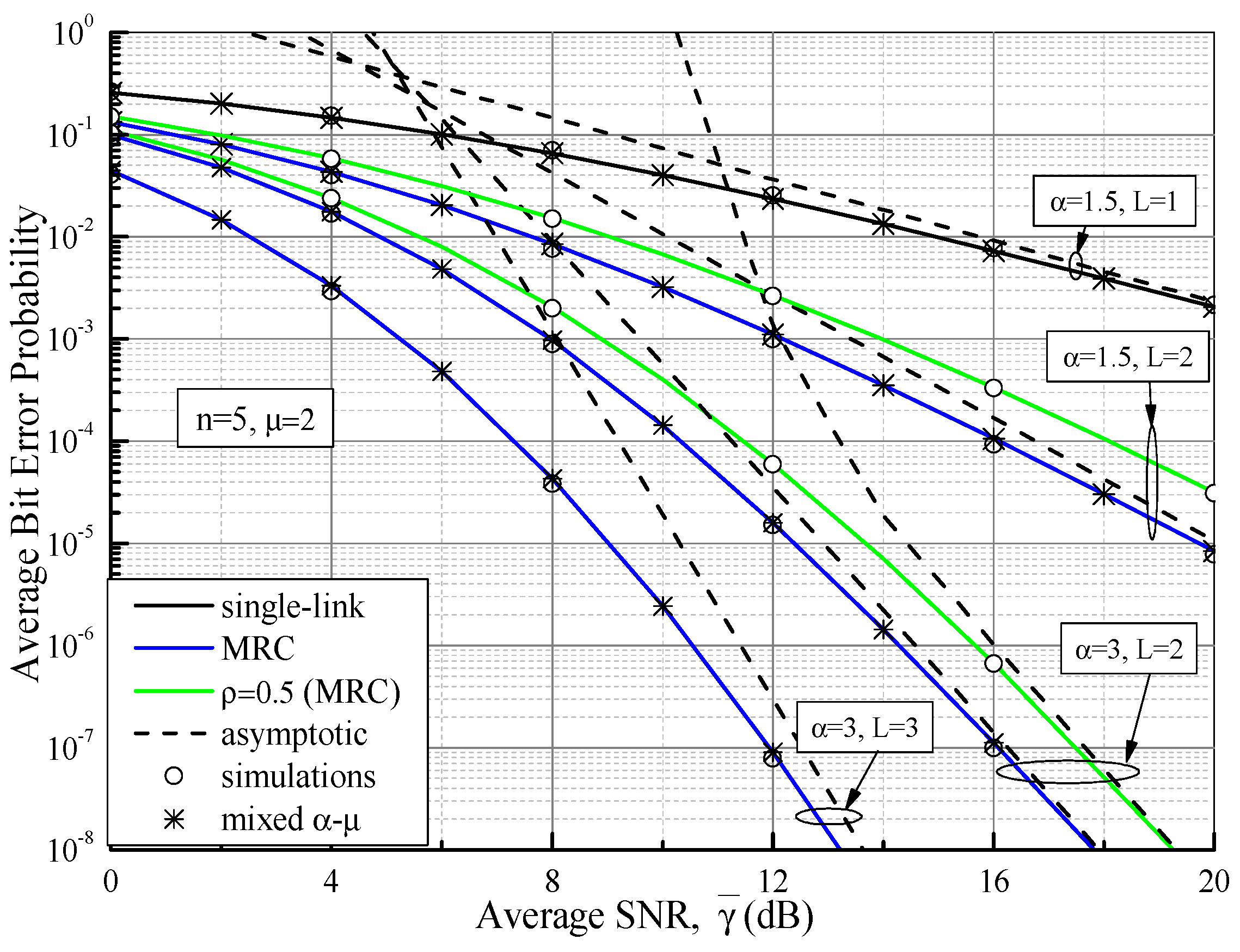
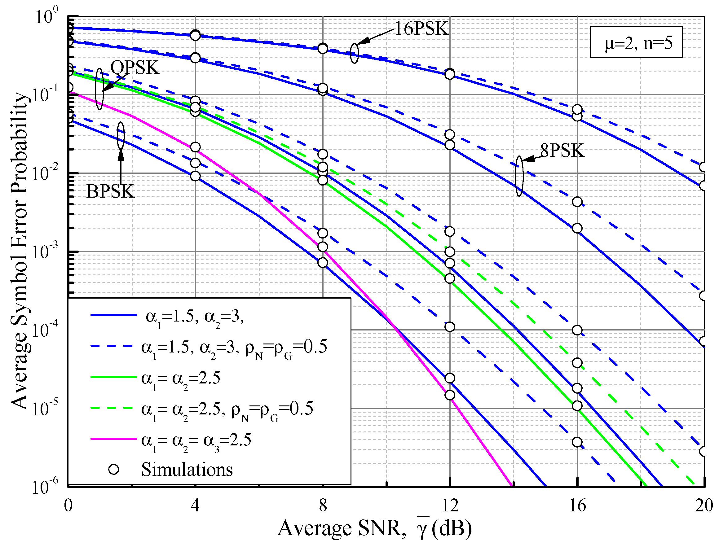
4.2. Average BEP/SEP

ABEP/ASEP is a conventional important measure to reveal the wireless communications system behaviors over fading environments. In the previous technical literature, two classical methods are often used to evaluate the ABEP/ASEP of various digital modulation schemes. One is the PDF-based approach, and the other is the MGF-based approach. In this paper, the former is considered and the unified conditional BEP/SEP formulas for several classical modulation schemes, such as DPSK, BPSK (Binary Phase Shift Keying), MPSK (M-ary PSK), and MQAM (Multiple Quadrature Amplitude Modulation), are summarized in terms of the exponential function form and the complementary error function form in

Table 2. Theoretical conditional BEP/SEP for several classical modulation schemes.

$\mathbf{BEP}/\mathbf{SEP}({\mathit{P}}_{\mathit{e}}(\mathit{\epsilon }|\mathit{\gamma }))$	Modulation Scheme	Parameter Values
$Aexp\left(-B\gamma \right)$	DPSK	$A=0.5,B=1$
$Cerfc\left(\sqrt{E\gamma }\right)-Derf{c}^2\left(\sqrt{E\gamma }\right)$	Coherent BPSK	$C=0.5,D=0,E=1$
	MPSK	$C=1, D=0,E={\sin }^2\left(\pi /\mathrm{M}\right),\mathrm{M}>4$
	Square MQAM	$C=2\left(1-1/\sqrt{\mathrm{M}}\right),$ $D={\left(1-1/\sqrt{\mathrm{M}}\right)}^2$, $E=1.5/\left(\mathrm{M}-1\right)$

, where $erfc(\ast )$ is the complementary error function defined in [37] (Equation (8.250.4)).

As is well-known, the ABEP/ASEP in fading environments can be obtained by averaging the conditional BEP/SEP ($P_e(\epsilon |\gamma )$ in Table 2) over the PDF ($f_{\gamma }\left(\gamma \right)$) of the instantaneous SNR ($\gamma$), namely

$$P_e(\epsilon )={\displaystyle {\int }_0^{\infty }{P}_e(\epsilon |\gamma )}{f}_{\gamma }(\gamma )d\gamma$$

(37)

Consequently, the ABEP/ASEP of the single-link and MRC systems in Section 2 and Section 3 can be deduced by substituting their corresponding PDFs into (37).

4.2.1. ABEP/ASEP in the Exponential Form

From Table 2, we can see the conditional BEP expressions of DPSK are written in the exponential form. For this case, the ABEP expressions for the single-link and MRC systems over independent and correlated fading channels can be derived by using the approaches to find the MGF of $\gamma$, such as (9). To this end, the exact ABEP expressions for various systems are obtained in

Table 3. ABEP expressions of DPSK for various systems.

Communication Systems	ABEP (Pe)
Single-link system by using (9)	$\frac{A\alpha }{2\mathsf{\Gamma }\left(\mu \right)\mathsf{\Gamma }\left(n\right)}{H}_{2,1}^{1,2}[\frac{\lambda }{B^{0.5\alpha }}{|}_{\left(\mu ,1\right)}^{\left(1-n,0.5\alpha \right),\left(1,0.5\alpha \right)}]$
Single-link system by using (12)	${\displaystyle \sum }_{i=1}^N\frac{A{\varsigma }_i\alpha }{2\mathsf{\Gamma }\left(\mu \right)}{H}_{1,1}^{1,1}[{\left(B{\psi }_i\right)}^{-0.5\alpha }{|}_{\left(\mu ,1\right)}^{\left(1,0.5\alpha \right)}]$
L-branch MRC system by using (A1)	$A{\displaystyle \prod }_{l=1}^L{A}_l{H}_{2,1}^{1,2}[\frac{{\lambda }_l}{B^{0.5{\alpha }_l}}{|}_{\left({\mu }_l,1\right)}^{\left(1-n_l,0.5{\alpha }_l\right),\left(1,0.5{\alpha }_l\right)}]$
L-branch MRC system by using (23)	${\displaystyle \sum }_{i_1=1}^{N_1}\cdots {\displaystyle \sum }_{i_L=1}^{N_L}A{\displaystyle \prod }_{l=1}^L\left(\frac{{\varsigma }_{i_l}{\alpha }_l}{2\mathsf{\Gamma }\left({\mu }_l\right)}{H}_{1,1}^{1,1}[{\left(B{\psi }_{i_l}\right)}^{-0.5{\alpha }_l}{|}_{\left({\mu }_l,1\right)}^{\left(1,0.5{\alpha }_l\right)}]\right)$
Two-branch MRC system by using (32)	${\displaystyle \sum }_{k=0}^{\infty }{\displaystyle \sum }_{l=0}^{\infty }\frac{0.25A\mathsf{\Phi }{\rho }_N^k{\rho }_G^l}{k!l!\mathsf{\Gamma }\left(k+\mu \right)\mathsf{\Gamma }\left(l+n\right)}{\displaystyle \prod }_{i=1}^2{H}_{2,1}^{1,2}[\frac{{\vartheta }_i}{B^{0.5{\alpha }_i}}{|}_{\left(\mu +k,1\right)}^{\left(1-n-l,0.5{\alpha }_i\right),\left(1,0.5{\alpha }_i\right)}]$

.

4.2.2. ABEP/ASEP in the Erfc Function Form

A. Single-Link System

By inserting $\mathit{Pe}(\epsilon |\gamma )$ in the erfc function form and (7) into (37), the ABEP/ASEP of the single-link system over α-μ/IGA fading channels can be given as

$$\begin{array}{cc}{P}_e(\epsilon )& =\frac{\alpha C}{2\mathsf{\Gamma }(\mu )\mathsf{\Gamma }(n)}\underset{I_3}{\underbrace{{\displaystyle {\int }_0^{\infty }{\gamma }^{-1}erfc(\sqrt{E\gamma })H_{1,1}^{1,1}[\lambda {\gamma }^{0.5\alpha }|{}_{(\mu ,1)}^{(1-n,0.5\alpha )}]d\gamma } }}\\ & -\frac{\alpha D}{2\mathsf{\Gamma }(\mu )\mathsf{\Gamma }(n)}\underset{I_4}{\underbrace{{\displaystyle {\int }_0^{\infty }{\gamma }^{-1}erf{c}^2(\sqrt{E\gamma })H_{1,1}^{1,1}[\lambda {\gamma }^{0.5\alpha }|{}_{(\mu ,1)}^{(1-n,0.5\alpha )}]d\gamma } }}.\end{array}$$

(38)

In order to solve the integrals (I₃ and I₄) in (38), we employ the identities [45] (Equations (8.4.14.2) and (8.3.2.21)) to represent the erfc function in terms of Fox’s H function as

$$erfc(\sqrt{E\gamma })={\pi }^{-0.5}{H}_{1,2}^{2,0}[E\gamma |{}_{(0,1),(0.5,1)}^{(1,1)}].$$

(39)

By inserting (39) into I₃ and I₄, with the help of [46] (Equation (2.8.4) and [47] (Equation (2.3)) and performing some algebraic operations, I₃ and I₄ can be obtained, respectively, as

$$I_3={\pi }^{-0.5}{H}_{3,2}^{1,3}[\lambda E^{-0.5\alpha }|{}_{(\mu ,1),(0,0.5\alpha )}^{(1-n,0.5\alpha ),(1,0.5\alpha ),(0.5,0.5\alpha )}],$$

$$I_4={\pi }^{-1}{H}_{2,1:1,2:1,1}^{0,2:2,0:1,1}[1,\lambda E^{-0.5\alpha }|{}_{(0,1,0.5\alpha )}^{(1,1,0.5\alpha ),(0.5,1,0.5\alpha )}|{}_{(0,1),(0.5,1)}^{(1,1)}|{}_{(\mu ,1)}^{(1-n,0.5\alpha )}].$$

(40)

Consequently, if we substitute (40) into (38), the exact ABEP/ASEP expression of the single-link system over α-μ/IGA fading channels can be obtained. Following the similar procedure used in (40) and utilizing (10), the exact approximated ABEP/ASEP expressions of the single-link system by using the mixed α-μ model can be deduced as

$$\begin{array}{cc}{P}_e(\epsilon )& ={\displaystyle \sum _{i=1}^N\frac{C\alpha {\pi }^{-0.5}{\varsigma }_i}{2\mathsf{\Gamma }(\mu )}{H}_{2,2}^{1,2}[{({\psi }_{i}E)}^{-0.5\alpha }|{}_{(\mu ,1),(0,0.5\alpha )}^{(1,0.5\alpha ),(0.5,0.5\alpha )}]}\\ & -{\displaystyle \sum _{i=1}^N\frac{D\alpha {\pi }^{-1}{\varsigma }_i}{2\mathsf{\Gamma }(\mu )}{H}_{2,1:1,2:0,1}^{0,2:2,0:1,0}[1,{({\psi }_{i}E)}^{-0.5\alpha }|{}_{(0;1,0.5\alpha )}^{(1;1,0.5\alpha ),(0.5;1,0.5\alpha )}|{}_{(0,1),(0.5,1)}^{(1,1)}|{}_{(\mu ,1)}^{-}]}\end{array}$$

(41)

B. MRC System

In the i.n.i.d. case, by inserting (20) into (37), a unified ABEP/ASEP formula in the erfc function form for an L-branch MRC system over α-μ/IGA fading channels can be expressed as

$$\begin{array}{cc}{P}_e(\epsilon )& =C{\pi }^{-0.5}{\mathsf{\Theta }}_1{H}_{1,1:{[2,1]}_{l=1:L}}^{0,1:{[1,2]}_{l=1:L}}[{\lambda }_1{E}^{-0.5{\alpha }_1},\cdots ,{\lambda }_L{E}^{-0.5{\alpha }_L}|{}_{(0;{\left\{0.5{\alpha }_l\right\}}_{l=1:L})}^{(0.5;{\left\{0.5{\alpha }_l\right\}}_{l=1:L})}|{}_{{[({\mu }_l,1)]}_{{}_{l=1:L}}}^{{[(1-n_l,0.5{\alpha }_l),(1,0.5{\alpha }_l)]}_{{}_{l=1:L}}}]\\ & -D{\pi }^{-1}{\mathsf{\Theta }}_1{H}_{2,2:{[2,1]}_{l=1:L}:1,2}^{0,2:{[1,2]}_{l=1:L}:2,0}[{\lambda }_1{E}^{-0.5{\alpha }_1},\cdots ,{\lambda }_L{E}^{-0.5{\alpha }_L},1|{}_{(1;{\left\{0.5{\alpha }_l\right\}}_{l=1:L},0),(0;{\left\{0.5{\alpha }_l\right\}}_{l=1:L},1)}^{(1;{\left\{0.5{\alpha }_l\right\}}_{l=1:L},1),(0.5;{\left\{0.5{\alpha }_l\right\}}_{l=1:L},1)}|{}_{{[({\mu }_l,1)]}_{{}_{l=1:L}}}^{{[(1-n_l,0.5{\alpha }_l),(1,0.5{\alpha }_l)]}_{{}_{l=1:L}}}|{}_{(0,1),(0.5,1)}^{(1,1)}].\end{array}$$

(42)

Proof: Please refer to Appendix B.

Similarly, by inserting (24) into (37), a unified ABEP/ASEP formula in the erfc function form for an L-branch MRC system by using the mixed α-μ model can also be obtained. In the correlated case, by inserting (33) into (37), a unified expression of ABEP/ASEP in the erfc function form for a two-branch MRC system over α-μ/IGA fading channels can be expressed as

$$\begin{array}{ll}{P}_e(\epsilon )& ={\displaystyle \sum _{k=0}^{\infty }{\displaystyle \sum _{l=0}^{\infty }\frac{0.25C{\pi }^{-0.5}\mathsf{\Phi }{\rho }_N^k{\rho }_G^l}{k!l!\mathsf{\Gamma }(k+\mu )\mathsf{\Gamma }(l+n)}{H}_{1,1:2,1:2,1}^{0,1:1,2:1,2}[{\vartheta }_1{E}^{-0.5{\alpha }_1},{\vartheta }_2{E}^{-0.5{\alpha }_2}{|}_{(0;0.5{\alpha }_1,0.5{\alpha }_2)}^{(0.5;0.5{\alpha }_1,0.5{\alpha }_2)}{|}_{(\mu +k,1)}^{(1,0.5{\alpha }_1),(1-n-l,0.5{\alpha }_1)}{|}_{(\mu +k,1)}^{(1,0.5{\alpha }_2),(1-n-l,0.5{\alpha }_2)}]}}\\ & -{\displaystyle \sum _{k=0}^{\infty }{\displaystyle \sum _{l=0}^{\infty }\frac{0.25D{\pi }^{-1}\mathsf{\Phi }{\rho }_N^k{\rho }_G^l}{k!l!\mathsf{\Gamma }(k+\mu )\mathsf{\Gamma }(l+n)}}}\\ & \times H_{2,2:2,1:2,1:1,2}^{0,2:1,2:1,2:2,0}[{\vartheta }_1{E}^{-0.5{\alpha }_1},{\vartheta }_2{E}^{-0.5{\alpha }_2},1{|}_{(1;0.5{\alpha }_1,0.5{\alpha }_2,0),(0;0.5{\alpha }_1,0.5{\alpha }_2,1)}^{(1;0.5{\alpha }_1,0.5{\alpha }_2,1),(0.5;0.5{\alpha }_1,0.5{\alpha }_2,1)}{|}_{(\mu +k,1)}^{(1,0.5{\alpha }_1),(1-n-l,0.5{\alpha }_1)}{|}_{(\mu +k,1)}^{(1,0.5{\alpha }_2),(1-n-l,0.5{\alpha }_2)}|{}_{(0,1),(0.5,1)}^{(1,1)}].\end{array}$$

(43)

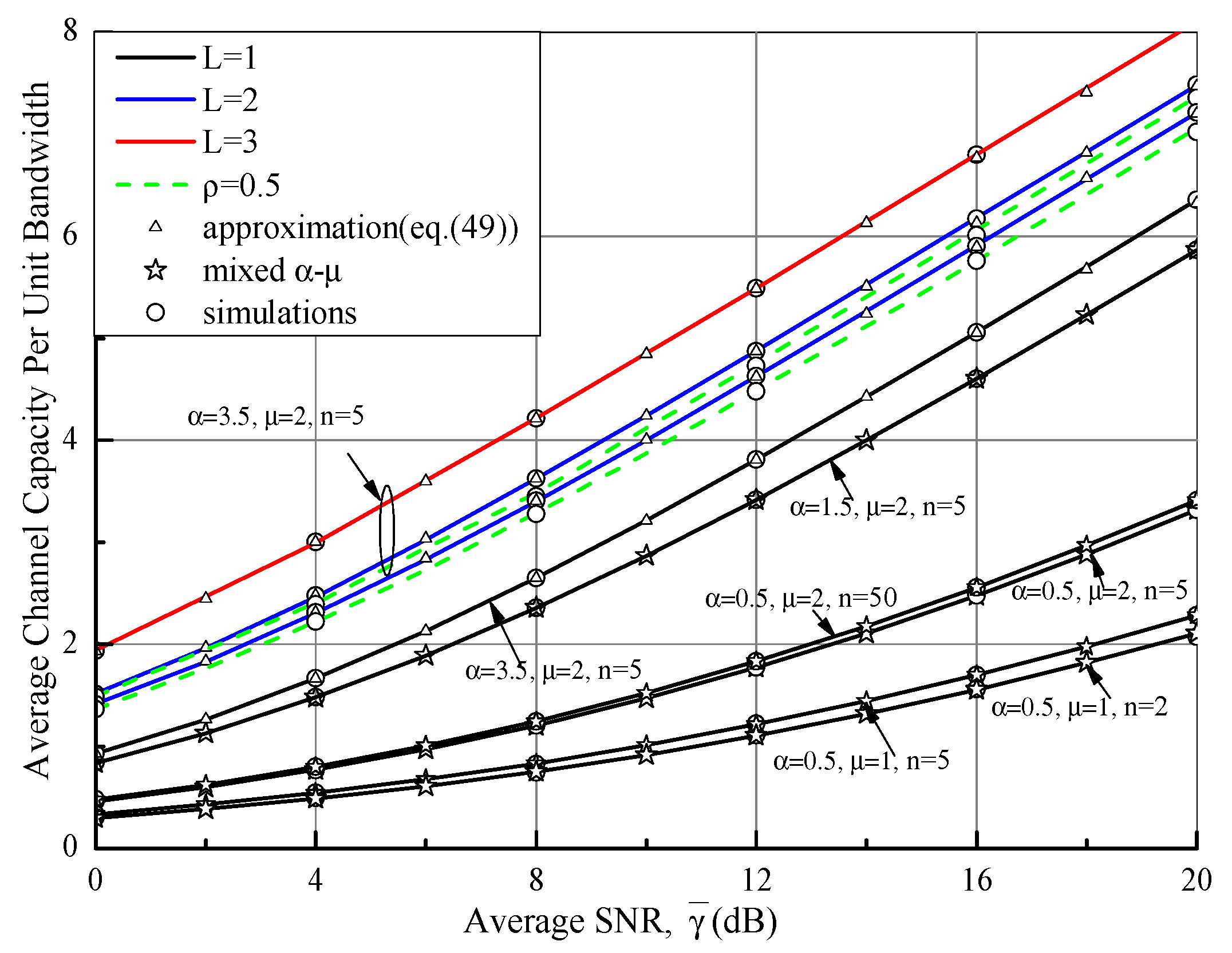
4.3. Average Channel Capacity

The channel capacity, in Shannon’s sense, is a core performance measure since it provides the maximum achievable transmission rate at which the errors are recoverable. The average channel capacity per unit bandwidth in fading channels can be expressed as

$${\overline{C}}_{\gamma }=\frac{B}{\ln 2}{\displaystyle {\int }_0^{\infty }\ln (1+\gamma )f_{\gamma }(\gamma )d\gamma },$$

(44)

where $f_{\gamma }\left(\gamma \right)$ is the PDF of the instantaneous SNR, $\gamma$.

4.3.1. Single-Link System

In order to find the closed-form expression of average channel capacity for the single-link system, we first use the identities in [45] (Equations (8.4.6.5) and (8.3.2.21)) to represent $\mathrm{l}\mathrm{n}\left(1+\gamma \right)$ in terms of Fox’s H-function as $H_{2,2}^{1,2}\left[\gamma {|}_{\left(1,1\right),\left(0,1\right)}^{\left(1,1\right),\left(1,1\right)}\right]$, then insert (7) into (44). After some mathematical manipulations, the exact expression of the average channel capacity for the single-link system over α-μ/IGA fading channels can be given by

$$\overline{C}=\frac{0.5\alpha }{\ln 2\mathsf{\Gamma }(\mu )\mathsf{\Gamma }(n)}{H}_{3,3}^{3,2}[\lambda |{}_{(\mu ,1),(0,0.5\alpha ),(0,0.5\alpha )}^{(1-n,0.5\alpha ),(0,0.5\alpha ),(1,0.5\alpha )}].$$

(45)

Similarly, by inserting (10) into (44), the exact approximate expression of the average channel capacity for the single-link system over α-μ/IGA fading channels can be obtained as

$$\overline{C}={\displaystyle \sum _{i=1}^N\frac{0.5{\varsigma }_i\alpha }{\ln 2\mathsf{\Gamma }(\mu )}{H}_{2,3}^{3,1}[{\psi }_i{}^{-0.5\alpha }|{}_{(\mu ,1),(0,0.5\alpha ),(0,0.5\alpha )}^{(0,0.5\alpha ),(1,0.5\alpha )}]}.$$

(46)

4.3.2. MRC System

In order to obtain the analytical expression of the average channel capacity of the MRC system and circumvent a mismatch with the definition of the multivariate H-function in [48,49], the final value theorem was adopted and an infinitesimal parameter close to zero was introduced. However, the multivariate H-function in the expression of Ergodic capacity in [48] (Equation (28)) did not exactly satisfy its definition in [38] (Equation (A.1)) because its parameter term was m = 1, not m = 0 as defined in [38] (Equation (A.1)). Moreover, the expression of Ergodic capacity in [49] (Equation (33)) avoided the above problem and caused a new case in which some associated coefficients ${\alpha }_j^{\left(i\right)}$ and ${\beta }_j^{\left(i\right)}$ defined in [49] (Equation (34)) are negative real numbers (e.g., −1), not positive real numbers as defined in [38] (Equation (A.5)). Therefore, by using the final value theorem and inserting (20) into (44) along with some mathematical manipulations, an exact expression of average channel capacity for the MRC system over α-μ/IGA fading channels can be derived as

$${\overline{C}}_{{\gamma }_{MRC}}=\left({\mathsf{\Theta }}_1/\ln 2\right)H_{1,1:{[2,1]}_{l=1:L}:2,2}^{0,1:{[1,2]}_{l=1:L}:1,2}[{\lambda }_1{s}^{-0.5{\alpha }_1},\cdots ,{\lambda }_L{s}^{-0.5{\alpha }_L},s^{-1}|{}_{(1;{\left\{0.5{\alpha }_l\right\}}_{l=1:L},0)}^{(1;{\left\{0.5{\alpha }_l\right\}}_{l=1:L},1)}|{}_{{[({\mu }_l,1)]}_{{}_{l=1:L}}}^{{[(1-n_l,0.5{\alpha }_l),(1,0.5{\alpha }_l)]}_{{}_{l=1:L}}}|{}_{(1,1),(0,1)}^{(1,1),(1,1)}],$$

(47)

where s is a very small positive number that goes to zero, for instance, s = 10⁻⁶. Similarly, by inserting (24) into (44), a unified expression of average channel capacity by using the mixed α-μ model can also be obtained. Unfortunately, it will take too long to calculate (47) in order to obtain the exact results in numerical analysis. To this end, an MGF-based method is also considered to evaluate the average channel capacity in this section. Thus, the average channel capacity per unit bandwidth can be given as [50] (Equation (8))

$${\overline{C}}_{{\gamma }_{MRC}}={(\ln 2)}^{-1}{\displaystyle {\int }_0^{\infty }{s}^{-1}[1-MG{F}_{{\gamma }_{MRC}}(s)]\exp (-s)ds}.$$

(48)

where $MG{F}_{{\gamma }_{MRC}}\left(s\right)$ is given in Equation (A1) in Appendix A. For the integral term in (48), it may be difficult to find an exact closed-form expression. By using the Gauss-Legendre quadrature method, the approximated form of (48) can be re-expressed as

$${\overline{C}}_{{\gamma }_{MRC}}={(\ln 2)}^{-1}{\displaystyle \sum _{i=1}^N{\omega }_i{t}_i^{-1}(1-MG{F}_{{\gamma }_{MRC}}(t_i))}.$$

(49)

For the correlated two-branch MRC system, based on the similar approach used in (47), by inserting (33) into (44), the average channel capacity per unit bandwidth over the correlated α-μ/IGA fading channels can be obtained as

$$\begin{array}{ll}{\overline{C}}_{{\gamma }_{MRC}}& ={\displaystyle \sum _{k=0}^{\infty }{\displaystyle \sum _{l=0}^{\infty }\frac{0.25{\left(\ln 2\right)}^{-1}\mathsf{\Phi }{\rho }_N^k{\rho }_G^l}{k!l!\mathsf{\Gamma }(k+\mu )\mathsf{\Gamma }(l+n)}}}\\ & \times H_{1,1:1,2:1,2:2,2}^{0,1:2,1:2,1:1,2}[{\vartheta }_1{s}^{-0.5{\alpha }_1},{\vartheta }_2{s}^{-0.5{\alpha }_2},s^{-1}{|}_{(1,0.5{\alpha }_1,0.5{\alpha }_2,0)}^{(1,0.5{\alpha }_1,0.5{\alpha }_2,1)}{|}_{(m+k,1)}^{(1,0.5{\alpha }_1),(1-n-l,0.5{\alpha }_1)}{|}_{(m+k,1)}^{(1,0.5{\alpha }_2),(1-n-l,0.5{\alpha }_2)}|{}_{(1,1),(0,1)}^{(1,1),(1,1)}].\end{array}$$

(50)

Similarly, the approximated form of the average channel capacity per unit bandwidth over the correlated α-μ/IGA fading channels is also obtained by inserting (32) into (49).

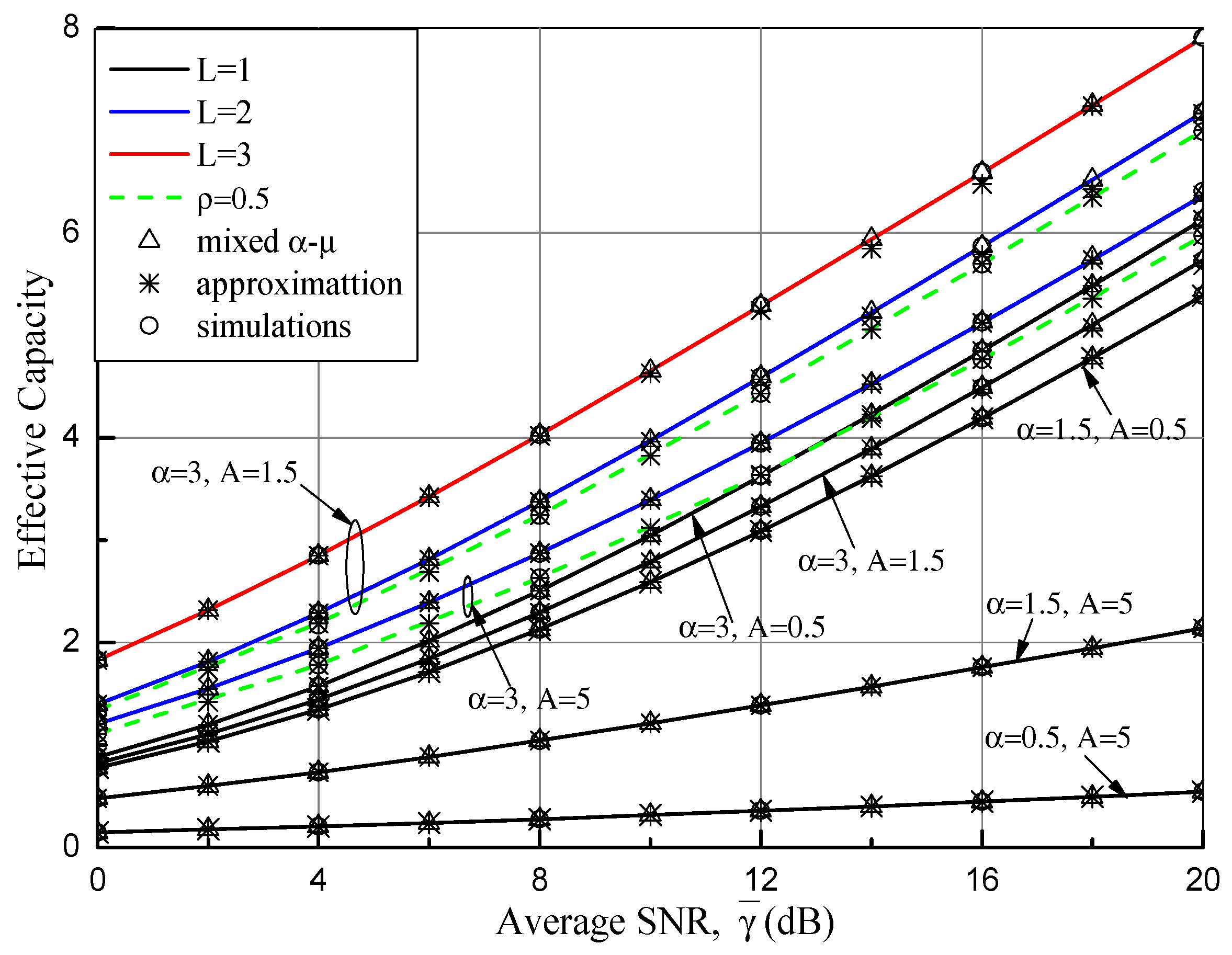
4.4. Effective Capacity

To evaluate the delay performance of some emerging wireless real-time applications under a quality of service (QoS) constraint, such as voice over IP and augmented reality/virtual reality, the effective capacity (EC), as an alternative performance metric of interest, has gained great attention. The EC is defined as the maximum constant arrival rate that a wireless fading channel can offer in a bid to ensure the QoS requirements. For wireless fading channels, the normalized EC can be expressed as

$$\Re =-\frac{1}{A}{\log }_2\left(\mathbb{E}\left[{(1+\gamma )}^{-A}\right]\right)=-\frac{1}{A}{\log }_2\left(\underset{I_5}{\underbrace{{\displaystyle {\int }_0^{\infty }{(1+\gamma )}^{-A}{f}_{\gamma }(\gamma )d\gamma } }}\right),$$

(51)

where $A=\theta TB⁄\ln 2$, $\theta$ denotes the QoS exponent characterizing the delay constraints, $T$ is the block length, $B$ represents the system bandwidth, and$f_{\gamma }\left(\gamma \right)$ is the PDF of the instantaneous SNR (γ).

4.4.1. Single-Link System

By substituting (7) into (51), the integral term I₅ in (51) can be yielded as

$$I_5=\frac{\alpha }{2\mathsf{\Gamma }(\mu )\mathsf{\Gamma }(n)}{\displaystyle {\int }_0^{\infty }{\gamma }^{-1}{(1+\gamma )}^{-A}{H}_{1,1}^{1,1}[\lambda {\gamma }^{0.5\alpha }|{}_{(\mu ,1)}^{(1-n,0.5\alpha )}]d\gamma }.$$

(52)

To solve the integral in I₅, we first represent ${\left(1+\mathsf{\gamma }\right)}^{-A}$ as $H_{1,1}^{1,1}\left[\mathsf{\gamma }{|}_{\left(0,1\right)}^{\left(1-\mathrm{A},1\right)}\right]/\mathsf{\Gamma }\left(\mathrm{A}\right)$ in terms of Fox’s H-function by using the identities in [45] (Equations (8.4.2.5) and (8.3.2.21)). Then with the aid of [46] (Equation (2.8.4)), after some mathematical manipulations, I₅ can be calculated as

$$I_5=\frac{\alpha }{2\mathsf{\Gamma }(\mu )\mathsf{\Gamma }(n)\mathsf{\Gamma }(A)}{H}_{2,2}^{2,2}[\lambda |{}_{(\mu ,1),(A,0.5\alpha )}^{(1-n,0.5\alpha ),(1,0.5\alpha )}].$$

(53)

Then, plugging (53) into (51), the exact expression of the effective capacity for the single-link system over α-μ/IGA fading channels can be obtained. When we substitute (10) into (51), the approximated expression of the effective capacity for the single-link system over the α-μ/IGA fading channels can be deduced as

$$\Re =-\frac{1}{A}{\log }_2\left({\displaystyle \sum _{i=1}^N\frac{0.5\alpha {\varsigma }_i}{\mathsf{\Gamma }(\mu )\mathsf{\Gamma }(A)}{H}_{1,2}^{2,1}[{\psi }_i{}^{-0.5\alpha }|{}_{(\mu ,1),(A,0.5\alpha )}^{(1,0.5\alpha )}]}\right).$$

(54)

4.4.2. MRC System

By inserting (20) into (51) and performing some similar manipulations as (52), the integral term I₅ in (51) can be derived as

$$I_5=\left({\mathsf{\Theta }}_1/\mathsf{\Gamma }(A)\right)H_{1,0:{[1,2]}_{l=1:L}}^{0,1:{[2,1]}_{l=1:L}}[1/{\lambda }_1,\cdots ,1/{\lambda }_L|{}_{-}^{(1-A;{\left\{0.5{\alpha }_l\right\}}_{l=1:L})}|{}_{{[(n_l,0.5{\alpha }_l),(0,0.5{\alpha }_l)]}_{{}_{l=1:L}}}^{{[(1-{\mu }_l,1)]}_{{}_{l=1:L}}}].$$

(55)

For the two-branch correlated case, by inserting (33) into (51), the integral term I₅ in (51) can be expressed as

$$\begin{array}{cc}{I}_5={\displaystyle \sum _{k=0}^{\infty }}{\displaystyle \sum _{l=0}^{\infty }}& \frac{0.25\mathsf{\Phi }{\rho }_N^k{\rho }_G^l{[\mathsf{\Gamma }(A)]}^{-1}}{k!l!\mathsf{\Gamma }(k+\mu )\mathsf{\Gamma }(l+n)}\\ & \times H_{1,0:1,2:1,2}^{0,1:2,1:2,1}[1/{\vartheta }_1,1/{\vartheta }_2{|}_{-}^{(1-A,0.5{\alpha }_1,0.5{\alpha }_2)}{|}_{(0,0.5{\alpha }_1),(n+l,0.5{\alpha }_1)}^{(1-\mu -k,1)}{|}_{(0,0.5{\alpha }_2),(n+l,0.5{\alpha }_2)}^{(1-\mu -k,1)}].\end{array}$$

(56)

Hence, the effective capacity for the MRC system over independent and correlated α-μ/IGA fading channels can be obtained by plugging (55) and (56) into (51), respectively. Similarly, by inserting (24) into (51), a unified expression of the effective capacity by using the mixed α-μ model can also be obtained. As an alternative approach to finding the analytical expression of the effective capacity, an MGF-based approach has been adopted [51]. Here, we employ the Gauss-Legendre quadrature method again, an alternative approximated form of (51) can be expressed as

$$\Re =-\frac{1}{A}{\log }_2\left(\frac{1}{\mathsf{\Gamma }(A)}{\displaystyle {\int }_0^{\infty }{x}^{A-1}\exp (-x)MG{F}_{\gamma }(x)dx}\right)=-\frac{1}{A}{\log }_2\left(\frac{1}{\mathsf{\Gamma }(A)}{\displaystyle \sum _{i=1}^N{\omega }_i{t}_i^{A-1}MG{F}_{\gamma }(t_i)}\right),$$

(57)

where $MG{F}_{\gamma }(\ast )$ can be obtained by using (9), (22), (32), and (A1).

5. Asymptotic Analysis

In the performance evaluation of wireless communication systems, the asymptotic analysis at the high average SNR level has been a popular evaluation methodology to observe how the channel parameters affect the performance and obtain more significant insights for system deployments. Generally, the diversity order and the coding gain are two performance metrics of interest to compare different modulation systems/fading models in the previous works. In high average SNR regions, the asymptotic OP or ABEP (ASEP) can be defined as ${\mathrm{P}}_x={\left(G_c·\overline{\gamma }\right)}^{-G_d}$, where $G_c$ denotes the coding gain, $G_d$ is the diversity order, and ${\mathrm{P}}_x$ represents the OP or ABEP/ASEP. In what follows, we will derive the asymptotic analytical expressions of the aforementioned communication systems over α-μ/IGA fading channels by taking the OP and the ABEP of DPSK as examples.

5.1. Single-Link System

As $\overline{\gamma }\to \infty ,$based on (7) and (8) with the aid of [46] (Th(1.11)), the asymptotic forms of the CDF and MGF for the single-link system can be obtained, respectively, as

$$F_{\gamma }(\gamma )\approx \frac{\mathsf{\Gamma }(n+0.5\alpha \mu )}{\mathsf{\Gamma }(1+\mu )\mathsf{\Gamma }(n)}{\left(\lambda {\gamma }^{0.5\alpha }\right)}^{\mu },$$

(58)

$$MGF(s)\approx \frac{\alpha \mathsf{\Gamma }(n+0.5\alpha \mu )\mathsf{\Gamma }(0.5\alpha \mu )}{2\mathsf{\Gamma }(\mu )\mathsf{\Gamma }(n)}{\left(\frac{\lambda }{s^{0.5\alpha }}\right)}^{\mu }.$$

(59)

Thus, by using (58) and (36), the asymptotic form of the OP for the single-link system can be expressed as

$$P_{out}\approx {\left(\frac{(n-1)}{\beta {\gamma }_{th}}{\left(\frac{\mathsf{\Gamma }(1+\mu )\mathsf{\Gamma }(n)}{\mathsf{\Gamma }(n+0.5\alpha \mu )}\right)}^{2/\alpha \mu }·\overline{\gamma }\right)}^{-0.5\alpha \mu }.$$

(60)

Similarly, from Table 3, the asymptotic form of the DPSK scheme for the single-link system can be derived as

$$Pe(\epsilon )\approx {\left(\frac{(n-1)B}{\beta }{\left(\frac{2\mathsf{\Gamma }(\mu )\mathsf{\Gamma }(n)}{A\alpha \mathsf{\Gamma }(n+0.5\alpha \mu )\mathsf{\Gamma }(0.5\alpha \mu )}\right)}^{2/\alpha \mu }·\overline{\gamma }\right)}^{-0.5\alpha \mu }.$$

(61)

5.2. MRC System

To obtain some useful insights into the MRC system as $\overline{\gamma }\to \infty$, by employing (59) and Equation (A1) in Appendix A, the asymptotic MGF of ${\gamma }_{MRC}$ in the i.i.d. case can be yielded as

$$MG{F}_{{\gamma }_{MRC}}(s)\approx {\left(\frac{\alpha \mathsf{\Gamma }(n+0.5\alpha \mu )\mathsf{\Gamma }(0.5\alpha \mu )}{2\mathsf{\Gamma }(\mu )\mathsf{\Gamma }(n){\lambda }^{-\mu }}\right)}^L{s}^{-0.5L\alpha \mu }.$$

(62)

Then, with the aid of the methods used in Equation (A3) in Appendix A, the asymptotic PDF of ${\gamma }_{MRC}$ in the i.i.d. case can be obtained as

$$f_{{\gamma }_{MRC}}(\gamma )\approx {\left(\frac{\alpha \mathsf{\Gamma }(n+0.5\alpha \mu )\mathsf{\Gamma }(0.5\alpha \mu )}{2\mathsf{\Gamma }(\mu )\mathsf{\Gamma }(n){\lambda }^{-\mu }}\right)}^L\frac{{\gamma }^{0.5L\alpha \mu -1}}{\mathsf{\Gamma }(0.5L\alpha \mu )}.$$

(63)

Thus, by integrating (63) with respect to $\gamma$ and using (36), the corresponding asymptotic OP of the MRC system, when $\overline{\gamma }\to \infty$, can be easily derived as

$$P_{out}\approx {\left({\left(\frac{2\mathsf{\Gamma }(\mu )\mathsf{\Gamma }(n){[\mathsf{\Gamma }(1+0.5L\alpha \mu )]}^{1/L}}{\alpha \mathsf{\Gamma }(n+0.5\alpha \mu )\mathsf{\Gamma }(0.5\alpha \mu )}\right)}^{2/\alpha \mu }\frac{(n-1)}{\beta {\gamma }_{th}}·\overline{\gamma }\right)}^{-0.5L\alpha \mu }.$$

(64)

Similarly, by using (62), the asymptotic ABEP of DPSK for the MRC system can be obtained as

$$P_e(\epsilon )\approx {\left(\frac{B(n-1)}{\beta A^{2/L\alpha \mu }}{\left(\frac{2\mathsf{\Gamma }(\mu )\mathsf{\Gamma }(n)}{\alpha \mathsf{\Gamma }(n+0.5\alpha \mu )\mathsf{\Gamma }(0.5\alpha \mu )}\right)}^{{}^{2/\alpha \mu }}·\overline{\gamma }\right)}^{-0.5L\alpha \mu }.$$

(65)

From the above asymptotic analysis, we can see that the diversity order of the single-link system is $0.5\alpha \mu$, and that of MRC systems is 0.5L$\alpha \mu$. As expected, the diversity systems can bring more benefits than the single-link system by the increase in the number of diversity branches. All the channel fading parameters show the impacts on the coding gain, while the diversity order depends on only the non-linear and the multipath parameters. Likewise, we can also derive the asymptotic expressions of the correlated cases and other modulation schemes and obtain some identical conclusions. In addition, the asymptotic results of the effective capacity can also be obtained at a high average SNR level by substituting (59) and (62) into (57).

6. Numerical and Simulation Results

To corroborate the derived analytical expressions in the previous sections, this section presents various numerical and simulation results under different α-μ/IGA fading channels. We adopted the Monte Carlo simulations to generate no less than 10e6 iterations. For the correlated scenarios, the simulation approaches described in [29] are considered by using a simple change of variables. In all figures, the simulation results provide a perfect matching with the numerical counterparts and confirm the availability of our theoretical derivations. In the numerical analysis, we provide some necessary methods to evaluate multivariate Fox’s H-functions and multiple-fold infinite/finite series sum in order to obtain accurate results. For the former, a Python code provided in [52] has been revised to compute them, such as (42) and (47). For the two-fold infinite series sum forms in the correlated cases, such as (43) and (50), we refer to the minimum numbers of truncated terms provided in [29] to meet the given target accuracy. Noted that k_min = l_min = 30 is considered for various values of the nonlinear parameter (α = 0.5, 1.5, 3.5) because it has similar effects on system performance as the multipath parameter (μ). Whereas for the finite series sum forms in (49), the number of terms (N) gradually increases as the average SNR ($\overline{\gamma }$) grows, for example, N = 30 as $\overline{\gamma }=10\mathrm{dB}$ and N = 150 as $\overline{\gamma }$ = 20 dB Even though the number of terms (N) is so large, it takes much less time to calculate (49) than (47) in order to get the same results. Finally, we consider some comparisons and discussions about the impacts of the non-linear parameter (α), the correlation coefficient ($\rho$), and the diversity branch (L) on the performance of different communication systems since the impacts of the multipath parameter (μ) and the shadowing parameter (n) on the performance have been profusely discussed in the previous works, such as [29,40,41,49].

In Figure 3 and Figure 4, we plot the OP of the single-link and MRC systems as a function of $\overline{\gamma }$ over α-μ/IGA fading channels with n = 5, μ = 2, and ${\gamma }_{th}$ = 5 dB, respectively. As anticipated, it can be observed that the OP of all the systems is improved when $\overline{\gamma }$ increases. In Figure 3, some performance comparisons are given in the i.i.d. case. It is clear that the OP gets better with the increase in the number of diversity branches (L = 1, 2, and 3), and the OP of MRC outperforms that of the single-link. Furthermore, the asymptotic results at the high average SNR region and the numerical results by using the mixed α-μ model are also presented, respectively. We can see that the former keeps tight with the exact results at the high average SNR level while the latter matches well with the exact results in the whole average SNR region with the truncated term N = 12. These results demonstrate the validity of our derivations. In Figure 4, some i.n.i.d. and correlated examples are considered. As expected, we can get some same conclusions as those in Figure 3. However, for the correlated cases, the OP of MRC degrades with the increase in the correlation coefficients ($\rho ={\rho }_N={\rho }_G$ = 0, 0.2, 0.5, and 0.7).

In Figure 5 and Figure 6, we illustrate the ABEP/ASEP of different modulation schemes for various communication systems as a function of the average SNR ($\overline{\gamma }$) over α-μ/IGA fading channels. In Figure 5, the ABEP of DPSK for various communication systems are compared under i.i.d. fading scenarios. It can be seen that the ABEP is improved when α (α = 1.5 and 3), the number of diversity branches (L = 1, 2, and 3), and the average SNR ($\overline{\gamma }$ = 0→20 dB) increases, respectively. Furthermore, the asymptotic results at the high average SNR region and the numerical results by using the mixed α-μ model also show similar behaviors as those in Figure 3. These results demonstrate the parameters α and L can provide the diversity gain, as shown in (64). In Figure 6, based on (42) and (43), we obtain the ASEP of MPSK for the MRC system in the i.n.i.d. and correlated cases. It is clear that the ASEP of MPSK degrades with the increase in the correlation coefficients ($\rho ={\rho }_N={\rho }_G$ = 0 and 0.5) and/or the order of modulation (M = 2, 4, 8, and 16).

Figure 7 plots the average channel capacity per unit bandwidth of various communication systems versus the average SNR ($\overline{\gamma }$) over several different communication conditions. It is evident that the average capacity improves with the growth of the value of α, μ, n, L, and/or $\overline{\gamma }$, respectively. However, the increase in $\rho$ $\left(\rho ={\rho }_N={\rho }_G\right)$ leads to the reduction in the average capacity. Interestingly, the growing trends of average capacity become slight when the value of n gets larger (n = 5→50) and/or when the value of $\rho$ gets smaller ($\rho =0.5\to 0$). These results suggest these parameters have less impact on the average capacity than other parameters (α, μ, L, and/or $\overline{\gamma }$). More importantly, the approximated analysis using (49) and the mixed α-μ model matches well with the exact numerical results. Moreover, Figure 8 shows the EC of various communication systems as a function of the average SNR ($\overline{\gamma }$) over several different communication conditions with n = 5 and μ = 2. It can be seen from Figure 8 that the EC gets larger with the increase in the value of α, L, and/or $\overline{\gamma }$, respectively. On the other hand, the EC gets smaller when the value of A and/or $\rho$ $\left(\rho ={\rho }_N={\rho }_G\right)$ grows, where the parameter A has a dominating impact on the EC. In addition, the approximated results by using (57) and the mixed α-μ model show good agreements with the exact numerical results.

7. Conclusions

In this paper, we presented a comprehensive investigation of the α-μ/IGA composite fading model and applied this model to the MRC system. First, we studied the fundamental statistics of the univariate and bivariate α-μ/IGA fading models including the PDF, CDF, and MGF, and proposed a mixture α-μ model to approximate the α-μ/IGA distribution. Then, as per the derived statistical expressions, the exact and approximated expressions of the statistical properties of the sum of α-μ/IGA variates by utilizing the multivariate Fox’s H-functions were obtained under the independent and the correlated fading environments. Third, some performance metrics of interest comprising the OP, ABEP/ ASEP, the average channel capacity, and the effective capacity were investigated in detail for the single-link and MRC systems, as well as their corresponding exact and approximated expressions, were derived in different channels conditions. Some asymptotic performance behaviors over α-μ/IGA fading were also provided in the high SNR regions. Finally, numerical analysis and Monte Carlo simulations were performed to prove the validity of the theoretical analysis under the different channel and system parameters. Our results will be helpful to improve the system reliability in the design and deployment of future communication applications, including 5G/6G wireless cellular systems, wearable communications, and vehicular wireless networks. Due to the simple and flexible form of the mixed α-μ model, we will apply it to other channel models and the complicated communication systems in future works, such as mmWave communications and Intelligent Reflecting Surface (IRS).

References

1. Simon, M.K.; Alouini, M.S. Digital Communication over Fading Channels, 2nd ed.; Wiley: Hoboken, NJ, USA, 2005. [Google Scholar]
2. Moualeu, J.M.; da Costa, D.B.; Lopez-Martinez, F.J.; de Souza, R.A.A. On the performance of α-η-κ-μ fading channels. IEEE Commun. Lett. 2019, 23, 967–970. [Google Scholar] [CrossRef]
3. Abdi, A.; Kaveh, M. K distribution: An appropriate substitute for Rayleigh-lognormal distribution in fading-shadowing wireless channels. Electron. Lett. 1998, 34, 851–852. [Google Scholar] [CrossRef] [Green Version]
4. Eltoft, T. The Rician inverse Gaussian distribution: A new model for non-Rayleigh signal amplitude statistics. IEEE Trans. Image Process. 2005, 14, 1722–1735. [Google Scholar] [CrossRef] [PubMed]
5. Bhatt, M.; Soni, S.K. A unified performance analysis of energy detector over α-η-μ/lognormal and α-κ-μ/lognormal composite fading channels with diversity and cooperative spectrum sensing. Int. J. Electron. Commun. (AEÜ) 2018, 94, 367–376. [Google Scholar] [CrossRef]
6. Al-Hmood, H.; Al-Raweshidy, H.S. Unified modeling of composite κ-μ/gamma, η-μ/gamma, and α-μ/gamma fading channels using a mixture gamma distribution with applications to energy detection. IEEE Antennas Wirel. Propag. Lett. 2017, 16, 104–108. [Google Scholar] [CrossRef]
7. Chauhan, P.S.; Soni, S.K. Average SEP and channel capacity analysis over Generic/IG composite fading channels: A unified approach. Phys. Commun. 2019, 34, 9–18. [Google Scholar] [CrossRef]
8. Paris, J.F. Statistical characterization of κ-μ shadowed fading. IEEE Trans. Veh. Technol. 2014, 63, 518–526. [Google Scholar] [CrossRef] [Green Version]
9. Simmons, N.; da Silva, C.R.N.; Cotton, S.L.; Sofotasios, P.C.; Yacoub, M.D. Double shadowing the Rician fading model. IEEE Wirel. Commun. Lett. 2019, 8, 344–347. [Google Scholar] [CrossRef]
10. Simmons, N.; Da Silva, C.R.N.; Cotton, S.L.; Sofotasios, P.C.; Yoo, S.K.; Yacoub, M.D. On shadowing the κ-μ fading model. IEEE Access 2020, 8, 120513–120536. [Google Scholar] [CrossRef]
11. Leonardo, E.J.; Yacoub, M.D. The product of two α-μ variates and the composite α-μ multipathshadowing model. IEEE Trans. Veh. Technol 2015, 64, 2720–2725. [Google Scholar] [CrossRef]
12. Badarneh, O.S. The α-μ/α-μ composite multipath-shadowing distribution and its connection with the extended generalized-K distribution. AEU-Int. J. Elect. Commun. 2016, 70, 1211–1218. [Google Scholar] [CrossRef]
13. Yoo, S.; Cotton, S.; Zhang, L.; Sofotasios, P. The inverse Gamma distribution: A new shadowing model. In Proceedings of the 8th Asia-Pacific Conference on Antennas and Propagation, Incheon, Korea, 4–7 August 2019; pp. 475–476. [Google Scholar] [CrossRef]
14. Ramırez-Espinosa, P.; Lopez-Martınez, F.J. On the utility of the inverse gamma distribution in modeling composite fading channels. In Proceedings of the IEEE Global Communications Conference, Waikoloa, HI, USA, 9–13 December 2019; pp. 1–6. [Google Scholar] [CrossRef] [Green Version]
15. Ramírez-Espinosa, P.; López-Martínez, F.J. Composite fading models based on inverse Gamma shadowing: Theory and validation. IEEE Trans. Wirel. Commun. 2021, 20, 5034–5045. [Google Scholar] [CrossRef]
16. Bithas, P.; Nikolaidis, V.; Kanatas, A.G.; Karagiannidis, G.K. UAV-to-ground communications: Channel modeling and UAV selection. IEEE Trans. Commun. 2020, 68, 5135–5144. [Google Scholar] [CrossRef]
17. Yoo, S.K.; Cotton, S.L.; Sofotasios, P.C.; Matthaiou, M.; Valkama, M.; Karagiannidis, G.K. The κ-μ/inverse gamma fading model. In Proceedings of the IEEE PIMRC, Hong Kong, China, 30 August–2 September 2015; pp. 425–429. [Google Scholar]
18. Yoo, S.K.; Sofotasios, P.C.; Cotton, S.L.; Matthaiou, M.; Valkama, M.; Karagiannidis, G.K. The η-μ/inverse gamma composite fading model. In Proceedings of the IEEE PIMRC, Hong Kong, China, 30 August–2 September 2015; pp. 166–170. [Google Scholar]
19. Yoo, S.K.; Bhargav, N.; Cotton, S.L.; Sofotasios, P.C.; Matthaiou, M.; Valkama, M.; Karagiannidis, G.K. The κ-μ/inverse gamma and η-μ/inverse gamma composite fading models: Fundamental statistics and empirical validation. IEEE Trans. Commun. 2017, 69, 5514–5530. [Google Scholar] [CrossRef]
20. Yoo, S.K.; Cotton, S.L.; Sofotasios, P.C.; Muhaidat, S.; Karagiannidis, G.K. Effective capacity analysis over generalized composite fading channels. IEEE Access 2020, 8, 123756–123764. [Google Scholar] [CrossRef]
21. Pant, D.; Chauhan, P.S.; Soni, S.K.; Naithani, S. BER and channel capacity analysis of wireless system over κ-μ/inverse gamma and η-μ/inverse gamma composite fading model. Wirel. Netw. 2021, 27, 1251–1267. [Google Scholar] [CrossRef]
22. Pant, D.; Chauhan, P.S.; Soni, S.K. Error probability and channel capacity analysis of wireless system over inverse gamma shadowed fading channel with selection diversity. Int. J. Commun. Syst. 2019, 32, e4083. [Google Scholar] [CrossRef]
23. Upaddhyay, V.K.; Chauhan, P.S.; Soni, S.K. Effective capacity analysis of SIMO system with MRC and SC over Inverse-Gamma shadowing. Int. J. Electron. 2021, 109, 181–199. [Google Scholar] [CrossRef]
24. Cheng, W.J.; Wang, X.T.; Xu, X.M. On the performance analysis of wireless transmission over α-μ/inverse gamma composite fading channels. In Proceedings of the IEEE/CIC International Conference on Communications in China (ICCC Workshops), Chongqing, China, 9–11 August 2020; pp. 64–69. [Google Scholar] [CrossRef]
25. Maurya, R.; Chauhan, P.S.; Srivastava, S.; Soni, S.K.; Mishra, B. Energy detection investigation over composite α-μ/inverse-Gamma wireless channel. Int. J. Electron. Commun. 2020, 130, 153556. [Google Scholar] [CrossRef]
26. Upaddhyay, V.K.; Soni, S.K.; Chauhan, P.S. An approximate statistical analysis of wireless channel over α-μ shadowed fading channel. Int. J. Commun. Syst. 2021, 34, e4884. [Google Scholar] [CrossRef]
27. Goswami, A.; Kumar, A. Statistical Characterization and Performance Evaluation of α−η−μ/Inverse Gamma and α−κ−μ/Inverse Gamma Channels. Wirel. Pers. Commun. 2022, 124, 2313–2333. [Google Scholar] [CrossRef]
28. Yoo, S.K.; Cotton, S.L.; Sofotasios, P.C.; Matthaiou, M.; Valkama, M.; Karagiannidis, G.K. The Fisher-Snedecor distribution: A simple and accurate composite fading model. IEEE Commun. Lett. 2017, 21, 1661–1664. [Google Scholar] [CrossRef] [Green Version]
29. Cheng, W.J.; Wang, X.T. Bivariate Fisher–Snedecor distribution and its applications in wireless communication systems. IEEE Access 2020, 8, 146342–146360. [Google Scholar] [CrossRef]
30. Cheng, W.J.; Wang, X.T.; Ma, T.F.; Wang, G. On the performance analysis of switched diversity combining receivers over Fisher–Snedecor composite fading channels. Sensors 2021, 21, 3014. [Google Scholar] [CrossRef]
31. Zhang, J.Y.; Du, H.Y.; Sun, Q.; Ai, B.; Ng, D.W.K. Physical layer security enhancement with reconfigurable intelligent surface-aided networks. IEEE Trans. Inf. Forensics Secur. 2021, 16, 3480–3495. [Google Scholar] [CrossRef]
32. Badarneh, O.S. The α- composite fading distribution: Statistical characterization and applications. IEEE Trans. Veh. Technol. 2020, 69, 8097–8106. [Google Scholar] [CrossRef]
33. Badarneh, O.S. The α-η- and α-κ- composite fading distributions. IEEE Commun. Lett. 2020, 24, 1924–1928. [Google Scholar] [CrossRef]
34. Badarneh, O.S.; Muhaidat, S.; Costa, D.B.D. The α-η-κ- composite fading distribution. IEEE Wirel. Commun. Lett. 2020, 9, 2182–2186. [Google Scholar] [CrossRef]
35. Treanta, S. Optimization on the distribution of population densities and the arrangement of urban activities. Stat. Optim. Inf. Comput. 2018, 6, 208–218. [Google Scholar] [CrossRef]
36. Yacoub, M.D. The α-μ distribution: A physical fading model for the stacy distribution. IEEE Trans. Veh. Technol. 2007, 56, 27–34. [Google Scholar] [CrossRef]
37. Gradshteyn, I.; Ryzhik, I. Table of Integrals, Series, and Products, 7th ed.; Academic: New York, NY, USA, 2007. [Google Scholar]
38. Mathai, A.M.; Saxena, R.K.; Haubold, H.J. The H-Function: Theory and Applications; Springer Science & Business Media: Berlin/Heidelberg, Germany, 2009. [Google Scholar]
39. Aldalgamouni, T.; Ilter, M.C.; Badarneh, O.S.; Yanikomeroglu, H. Performance analysis of fisher-snedecor composite fading channels. In Proceedings of the IEEE Middle East and North Africa Communications Conference, Jounieh, Lebanon, 18–20 April 2018; pp. 1–5. [Google Scholar] [CrossRef]
40. Al-Hmood, H.; Al-Raweshidy, H.S. Selection combining scheme over non-identically distributed Fisher-Snedecor fading channels. IEEE Wirel. Commun. Lett. 2021, 10, 840–843. [Google Scholar] [CrossRef]
41. Badarneh, O.S.; Costa, D.B.D.; Sofotasios, P.C.; Muhaidat, S.; Cotton, S.L. On the sum of Fisher-Snedecor variates and its application to maximal-ratio combining. IEEE Wirel. Commun. Lett. 2018, 7, 966–969. [Google Scholar] [CrossRef] [Green Version]
42. Atapattu, S.; Tellambura, C.; Jiang, H. A mixture gamma distribution to model the SNR of wireless channels. IEEE Trans. Wirel. Commun. 2011, 10, 4193–4203. [Google Scholar] [CrossRef]
43. Ramirez-Espinosa, P.; Moualeu, J.M.; da Costa, D.B.; Lopez-Martinez, F.J. The α-κ-μ shadowed fading distribution: Statistical characterization and applications. In Proceedings of the IEEE Global Communications Conference, Waikoloa, HI, USA, 9–13 December 2019; pp. 1–6. [Google Scholar] [CrossRef] [Green Version]
44. Bithas, P.S.; Kanatas, A.G.; Matolak, D.W. Exploiting shadowing stationarity for antenna selection in V2V communications. IEEE Trans. Veh. Technol. 2018, 68, 1607–1615. [Google Scholar] [CrossRef]
45. Prudnikov, A.P.; Brychkov, Y.A.; Marichev, O.I. Integrals and Series (More Special Functions); Gordon and Breach: Philadelphia, PA, USA, 1992; Volume 3. [Google Scholar]
46. Kilbas, A.A.; Saigo, M. H-Transforms: Theory and Applications (Analytical Method and Special Function), 1st ed.; Chapman & Hall/CRC Press: Boca Raton, FL, USA, 2004. [Google Scholar] [CrossRef]
47. Mittal, P.K.; Gupta, K.C. An integral involving generalized function of two variables. Proc. Indian Acad. Sci.-Sect. A 1972, 75, 117–123. [Google Scholar] [CrossRef]
48. Rahama, Y.A.; Ismail, M.H.; Hassan, M. On the sum of independent Fox’s H-Function variates with applications. IEEE Trans. Veh. Technol. 2018, 67, 6752–6760. [Google Scholar] [CrossRef]
49. Du, H.Y.; Zhang, J.Y.; Cheng, J.L.; Ai, B. Sum of Fisher-Snedecor random variables and its applications. IEEE Open J. Commun. Soc. 2020, 1, 342–356. [Google Scholar] [CrossRef]
50. Hamdi, K.A. Capacity of MRC on correlated rician fading channels. IEEE Trans. Commun. 2008, 56, 708–711. [Google Scholar] [CrossRef] [Green Version]
51. Ji, Z.; Dong, C.; Wang, Y.; Lu, J. On the analysis of effective capacity over generalized fading channels. In Proceedings of the IEEE International Conference on Communications, Sydney, Australia, 10–14 June 2014; pp. 1977–1983. [Google Scholar] [CrossRef]
52. Alhennawi, H.R.; El Ayadi, M.M.; Ismail, M.H.; Mourad, H.A.M. Closed-form exact and asymptotic expressions for the symbol error rate and capacity of the H-function fading channel. IEEE Trans. Veh. Technol. 2016, 65, 1957–1974. [Google Scholar] [CrossRef]
Figure 1. PDFs of the α-μ/IGA and α- F models for different channel parameters with γ ¯ = 1 .
Applsci 12 05375 g001
Figure 2. Impacts of different system and channel parameters on the exact PDF in (7), the mixed α-μ PDF in (10), and the mixed IGA PDF in (13).
Applsci 12 05375 g002
Figure 3. Outage probability of various communication systems as a function of the average SNR over i.i.d. α-μ/IGA fading channels with n = 5, μ = 2, and γ t h = 5 dB.
Applsci 12 05375 g003
Figure 4. Outage probability of various communication systems as a function of the average SNR ( γ ¯ ) over i.n.i.d. and correlated α-μ/IGA fading channels with n = 5, μ = 2, and γ t h = 5 dB.
Applsci 12 05375 g004
Figure 5. ABEP of DPSK for various communication systems as a function of the average SNR ( γ ¯ ) over i.i.d. α-μ/IGA fading channels with n = 5 and μ = 2.
Applsci 12 05375 g005
Figure 6. ASEP of MPSK for the MRC system as a function of the average SNR ( γ ¯ ) over i.n.i.d. and correlated α-μ/IGA fading channels with n = 5 and μ = 2.
Applsci 12 05375 g006
Figure 7. Average channel capacity per unit bandwidth of various communication systems as a function of the average SNR ( γ ¯ ) over different α-μ/IGA fading channels.
Applsci 12 05375 g007
Figure 8. Effective capacity of various communication systems as a function of the average SNR ( γ ¯ ) over different communication conditions with n = 5 and μ = 2.
Applsci 12 05375 g008