Featured Application
The proposed methodology enables researchers and sport scientists to compare and evaluate NFL drafts based on the evaluation of experts. Additionally, it offers an easy-to-use and reliable solution to solve multicriteria decision making problems, commonly found in sport sciences.
Abstract
Predicting the success of National Football League drafts has always been an exciting issue for the teams, fans and even for scientists. Among the numerous approaches, one of the best techniques is to ask the opinion of sport experts, who have the knowledge and past experiences to rate the drafts of the teams. When asking a set of sport experts to evaluate the performances of teams, a multicriteria decision making problem arises unavoidably. The current paper uses the draft evaluations of the 32 NFL teams given by 18 experts: a novel multicriteria decision making tool has been applied: the sum of ranking differences (SRD). We introduce a quick and easy-to-follow approach on how to evaluate the performance of the teams and the experts at the same time. Our results on the 2021 NFL draft data indicate that Green Bay Packers has the most promising drafts for 2021, while the experts have been grouped into three distinct groups based on the distance to the hypothetical best evaluation. Even the coding options can be tailored according to the experts’ opinions. Statistically correct (pairwise or group) comparisons can be made using analysis of variance (ANOVA). A comparison to TOPSIS ranking revealed that SRD gives a more objective ranking due to the lack of predefined weights.
1. Introduction
The National Football League (NFL) draft is held yearly, between the Super Bowl and the start of the season, resulting in teams signing college players. The first NFL draft was organized in 1936, as previously the richer teams had been allowed to select young players, so the competition was unbalanced. With the introduction of the NFL draft, the competition became more balanced, with teams with poorer records being able to pick better players. The draft involves 32 teams who sign the best college players in the country. During the draft, the 32 NFL teams have the opportunity to select American college players. Each player can only be selected by one team. There are multiple rounds of picks, each consisting of as many picks as there are teams in the draft, for a total of 32. In 2020, there were 255 picks in seven rounds, while in 2021 there were 224 picks in seven rounds (https://www.nfl.com (accessed on 14 June 2022)).
Wolfson et al. [1] addressed the backward prediction problem. Their analysis showed that college and combine statistics have little value in predicting whether a quarterback will be successful in the NFL. The NFL Combine is held annually and is held about two months before the draft. It assesses players’ physical and mental abilities. The authors obtained draft position and most NFL statistical data from: https://www.pro-football-reference.com/ (accessed on 14 June 2022) for quarterbacks drafted between 1997 and 2009. Combine data were obtained from http://draftscout.com/ (accessed on 14 June 2022). For each regression, two primary models were considered: the first model, called Base, contains the predictors and Draft Year, and the second model contains the Base predictors and log (Pick) values, which show where players were selected in the draft. They conclude that NFL teams aggregate pre-draft information quite efficiently and are unable to consistently identify college quarterbacks who will excel among the pros, a consequence of random variability in future performance due to factors that are unobservable, uncontrollable, and very likely.
Mulholland and Jensen [2] created a separate predictive model focusing on the tight end position. The reason for this is that the NFL is increasingly moving towards a pass-oriented league, so it is necessary to examine the tight end position, too. The model was created for the NFL draft and NFL career performance based on available data from the pre-draft period (college performance, NFL combine, physical measures). Linear regression and recursive partitioning decision trees were used. Using both modelling approaches, they found that the measures that best predict NFL draft order are not necessarily the measures that best predict NFL career success. This finding indicates that the current draft strategy for tight ends can (and should) be improved.
In 2016, Becker and Sun [3] studied fantasy football based on actual NFL player performance. Becker and Sun set out to create a method that predicts team and player performances based on historical data, i.e., to develop a method that provides a comprehensive optimization strategy for the entire season. A model that could quickly perform the task to be solved was needed, keeping in mind that during the draft, teams have a short time (1–3 min) to make a choice. In the study, they found that the probability of winning money with the IP drafting approach was statistically significantly higher than with the baseline approach at a 99.75% confidence level after running 300 simulation tests.
The sum of ranking differences (SRD) method was introduced for fair method and model comparison providing a unique one-dimensional ranking of methods and/or models in 2010 [4]. SRD was primarily developed to solve method-comparison problems in a fast, easy way by creating a clear rank of subjects based on comparison with an ideal ranking (benchmark). Interpretation of the results is also simple: the smaller the SRD, the better the method, i.e., it is closer to the gold standard (benchmark). Validation was done by comparing the ranking of the input matrix to SRD ranks obtained from random numbers. In the last decade, SRD has been continuously improved and new features have been incorporated. The first improvement was to develop a strict mathematical validation method for the SRD scores. When the number of random matrices is large enough, a distribution is obtained by Monte Carlo simulation and can be used to determine if the ranks of the input matrix are significantly different from random ranking (i.e., the original variables overlap with the distribution of random variables). The approach was called compare ranks with random numbers (CRRN) and was introduced in 2011 [4]. With CRRN, the authors introduced the concept of theoretical SRD distribution, described as a broken asymmetric one, and revealed the differences for various sample sizes. However, the discrete distribution can be approximated with high accuracy if the number of rows in the input matrix exceeds 13 [4]. The next step was to solve the problem of ties, e.g., the presence of repeated observations, which occur frequently if the same ranking is given to two or more variables. Handling ties required an algorithm to define the new theoretical SRD distributions. For sample sizes between four and nine (4 < n < 9), exact theoretical distributions are used, but in the case of n > 8, Gaussian approximation, fitted on the SRD distribution and generated using three million n–dimensional random vectors, gives a high quality approximation [5].
Recent examinations clearly and unambiguously have shown that sum of ranking differences (SRD) realizes a multicriteria decision making (MDCM) tool [6,7]. Moreover, it was proven that SRD provides the consensus of eight independent MCDM tools [7]. The other validation possibility for SRD is cross-validation [5,8]: the evaluation of the effects of different SRD validation variants such as the ways of cross-validations (contiguous n-fold and repeated resampling with return). The number of folds (five-, six-, seven-, eight-, nine-, and tenfold) was selected as the recommended optimum [9].
Currently, SRD has been made available on different platforms out of Microsoft Excel VBA. A python-based (https://github.com/davidbajusz/srdpy (accessed on 14 June 2022)), and a platform-independent version (https://attilagere.shinyapps.io/srdonline/ (accessed on 14 June 2022)) are also available with some limitations.
MATLAB codes are also available to perform sum of ranking differences at: https://www.isu.edu/chem/faculty/staffdirectoryentries/kalivas-john.html (accessed on 14 June 2022) in base form: 2013_12_16_SRD.7z, and to perform single-class fusion classification with SRD: 2019_11_25_SingleClassCode.7z.
The visualization is also enhanced by a modification of an arrangement of SRD lines and coupled with parallel coordinates. The MATLAB and Octave codes and test data of environmental relevance are accessible at https://github.com/abonyilab/parcoord (accessed on 14 June 2022).
Due to its flexibility and ease of use, SRD has been used in different fields of science such as eye-tracking [10]; food science [11]; column selection in chromatography [12,13]; variable selection [14]; ordering and grouping octanol-water (logP) partition coefficient determination methods [15,16]; selection of edible insects based on nutritional composition [17]; outlier detection in multivariate calibration [18]; non-parametric ranking of QSAR models [19]; comparison of ensemble learning models [20]; comparison of tea grade identification using electronic tongue data [21]; testing the outer consistency of novel similarity indices [22]; and even ranking of sportsmen [23], just to name a few.
The present work is devoted to analyzing the 2021 NFL draft evaluations given by 18 experts to test the consistency of their rankings.
2. Materials and Methods
2.1. Data Set
The data set compiled by René Bugner: https://twitter.com/RNBWCV/status/1388864754450567169/photo/1 (accessed on 14 June 2022) contains the draft evaluation of the 32 NFL teams given by 18 experts. Their names and coding are gathered in Table 1 together with the coding of teams.

Table 1.
Coding of experts and teams.
2.2. Sum of Ranking Differences
2.2.1. Evaluation of Experts
Sum of ranking differences (SRD) as a multicriteria optimization method is able to compare the evaluation of 18 draft experts based on their scores given to the teams. As we currently do not know a theoretically best ranking (e.g., which expert(s) has (have) the perfect draft ranking), SRD uses their consensus (data fusion). SRD has multiple options for the definition of the theoretically best ranking including minimum, maximum, average, and any user-defined reference. Minimum, maximum, and average values are calculated row-wise, while user defined vectors are provided by the users. Consensus modeling is used for multicriteria decision making problems, even if the preference structures are different. The consensus is characterized by indicators showing the agreement between experts’ opinions. Similarly, a measure of proximity is defined to find out how far the individual opinions are from the group opinion [24]. However, the expert opinion is interchangeable to any kind of modeling method. Consensus modeling is frequently bounded with data fusion [25] and is also common in quantitative structure-activity relationships modeling [26].
SRD ranks the teams based on the scores given by the experts, therefore each expert gets a vector of ranks from 1 to 32, as 32 teams are considered. In the second step, the so-called reference column, which is the consensus of all 18 experts, is also ranked from 1 to a maximum of 32 (one is the worst, two is the second worst, and so on, the largest is the best). The third step involves the computation of the row-wise rank differences between each expert and the reference column. The absolute rank differences are then summed up for each expert, creating the sum of ranking differences, a single demonstration of the distance between an expert and the consensus. If the SRD value of an expert equals zero, the expert ranked the teams exactly as the average of all experts’ scores (consensus). Median is also a viable option to define a consensus, it is warranted if outlying observations are suspected. Higher SRD values mean higher deviations from the consensus. Patterns of SRDs therefore might suggest characteristic groupings among the variables, e.g., variables closer to each other are more similar in terms of their distance from the reference. The algorithm for the sum of ranking differences was calculated with Microsoft Office Excel 2007 macro retrieved from: http://aki.ttk.hu/srd/ (accessed on 14 June 2022).
The next type of validation of the SRD values was by ANOVA with Factor 1: resampling variant (two levels: contiguous sevenfold resampling–A, random resampling with replacement–B), Factor 2: coding (two levels: (1) GPA coding, (2) partial reverse coding (full ranking): 14 categories from A− to F− are stretched from 1 to 32, and C), and Factor 3: experts (18 levels).
The first validation is the randomization test, it shows the distance (probability of) from random ranking.
2.2.2. Evaluation of Teams
First, the input matrix was transposed, therefore the teams were presented in columns, while the experts were presented in the rows. The data has been rank-transformed column-wise, where the lowest GPA score received the lowest rank (1), while tied scores received averaged ranks. The Factor 1 was the same as earlier: cross-validation variants, two levels A and B, Factor 2: two levels (1) GPA Coding, and (2) preserving the 14 categories, Factor 3: 32 levels, i.e., the teams.
2.2.3. Coding of Data
The original data set provided by René Bugner uses the GPA system which ranges from F− to A+ on the presented data set. The 4+ coding system was used to convert the GPA letters to numbers, which range from 0 (F−) to 4.3 (A+). The reason behind choosing the 4+ system instead of the more common 4-point system is that the experts used mainly the upper part of the GPA scale, meaning that multiple A’s and A+’s are used in their evaluations; therefore the 4+ system enables a better discrimination of the teams. The coding is denoted by GPAraw.
However, a different coding has also been applied in order to highlight the differences between the teams even more. GPA codes were transferred to ranks, the average of 4+ system numbers were used for equal codes (partial ranking) denoted by GPAreRank.
3. Results
3.1. Evaluation of Experts
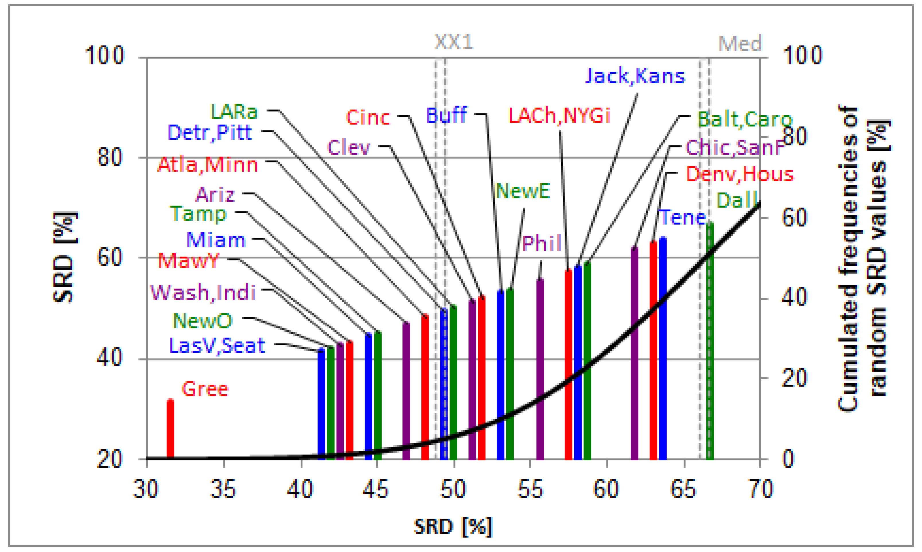
Results based on the 4+ GPA conversion system are presented by Figure 1. The SRD plot compares the experts to a reference column, defined as maximum here. The rationale behind choosing the maximum column as a benchmark is equivalent to define a hypothetical best expert, who can always select the best team. The plot presents a tangent hyperbolic curve, approximating the cumulated Gaussian distribution function of the random SRD values. Rankings placed on the left side of the XX1 range (5%) mean significant rankings (the probability of random ranking is less than 5%). As we look at the plot, some differentiation can clearly be seen. There is a smaller group of experts who are more optimistic regarding the 2021 drafts: RF, RD, TB, LE, FS, and St1 when compared to the others, as their SRD scores are closer to the zero SRD point.
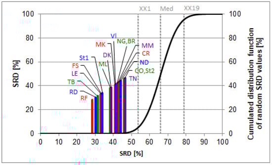
Figure 1.
The SRD values (scaled between 0 and 100) of the experts based on their ratings determined by sum of ranking differences. Maximum values were used as the reference (benchmark) column, which had the highest scores. Scaled SRD values are plotted on the x axis and left y axis, right y axis shows the relative frequencies of random ranking distribution function: black curve. The probability ranges are also given as 5% (XX1), Median (Med), and 95% (XX19). Codes of the experts are listed in the data set section.
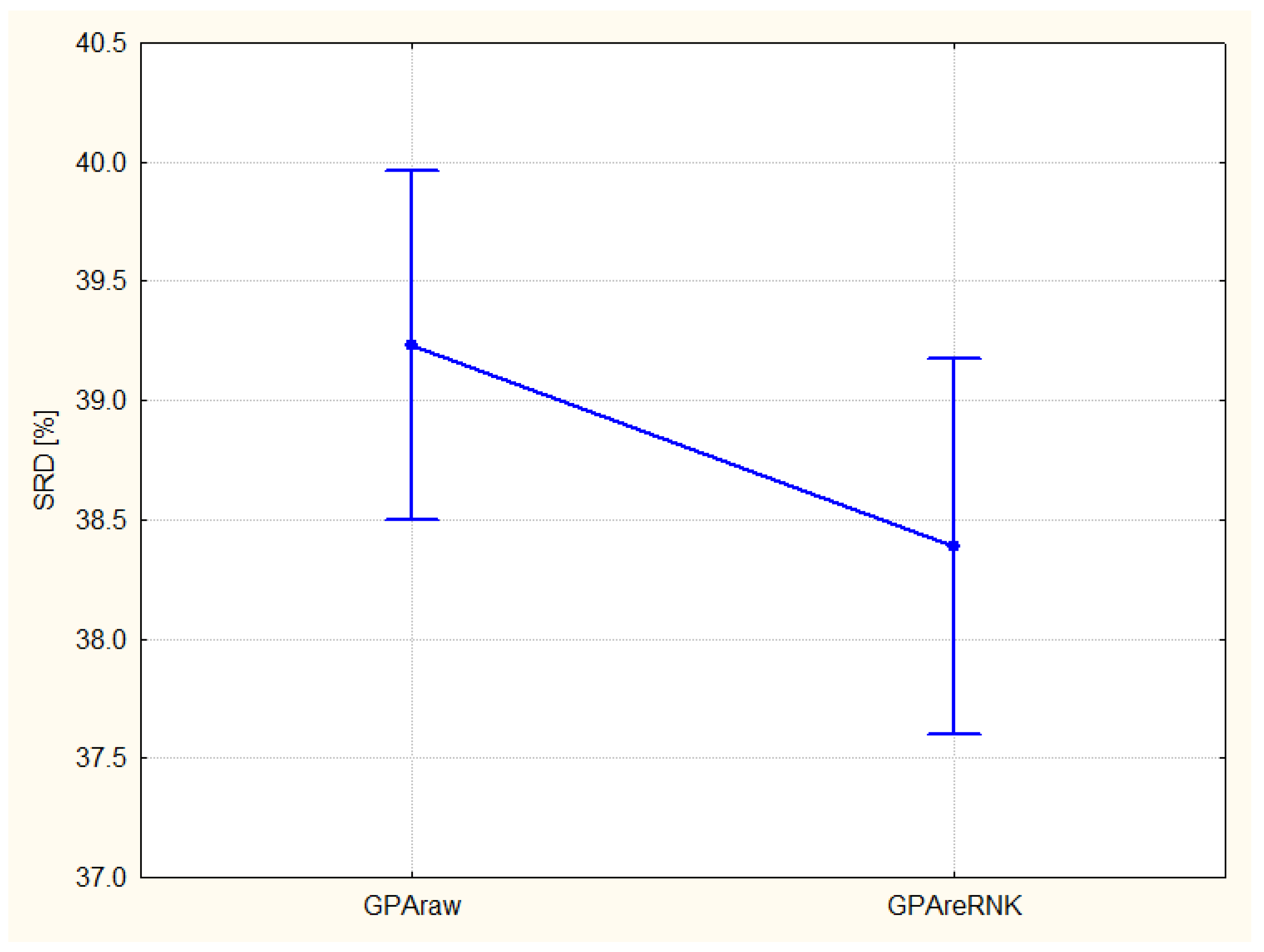
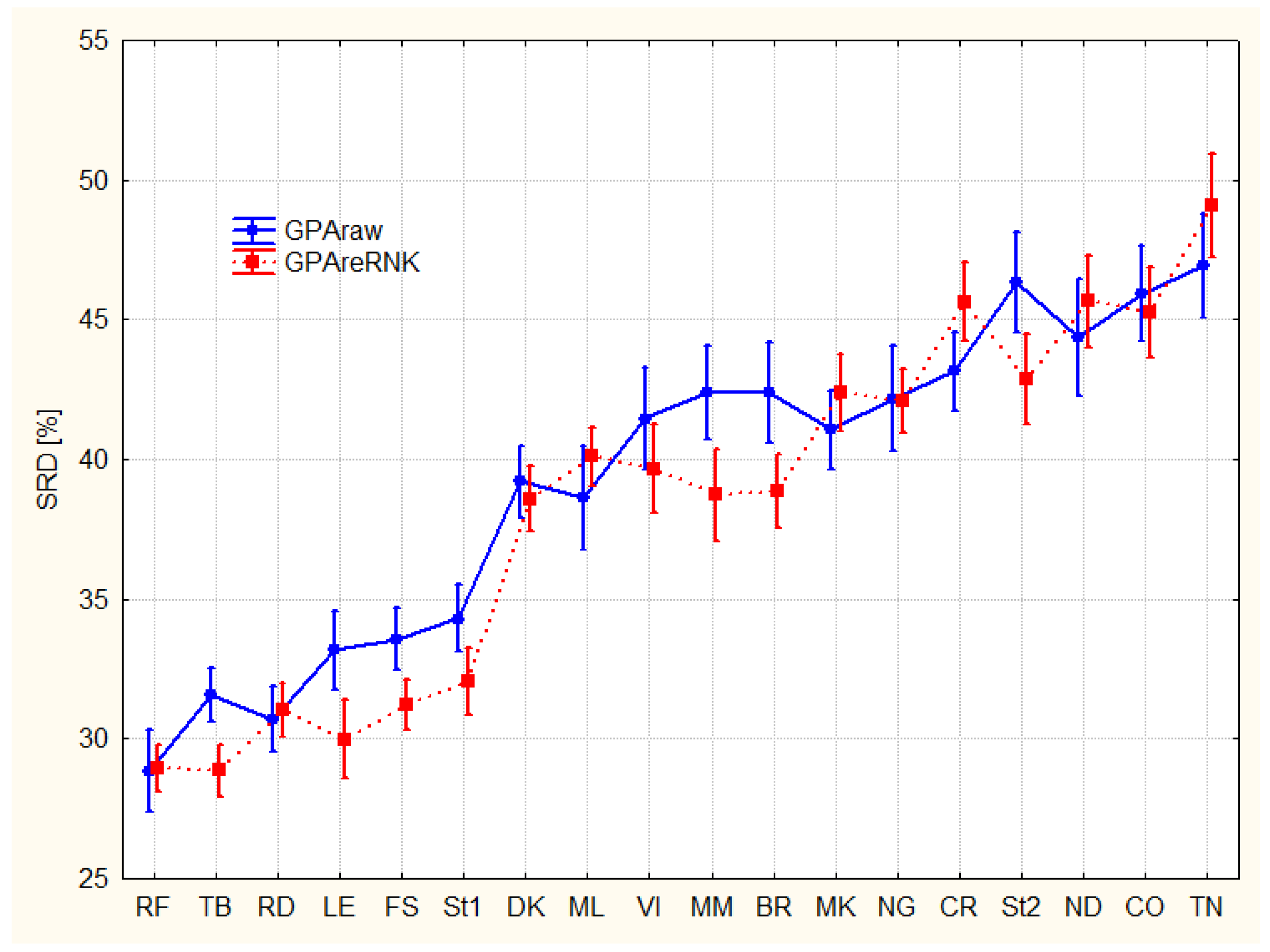
Factorial ANOVA decomposes the effects of the various factors and their couplings. The Figure 2 shows the differences in coding, the original GPA rank is inferior to the full ranking (the smaller the SRD the better).

Figure 2.
Comparison of coding options GPAraw–original GPA coding, GPAreRank (recoding to full rank) error bars represent 95% confidence interval. The variances are homogeneous according to the Levene’s test.
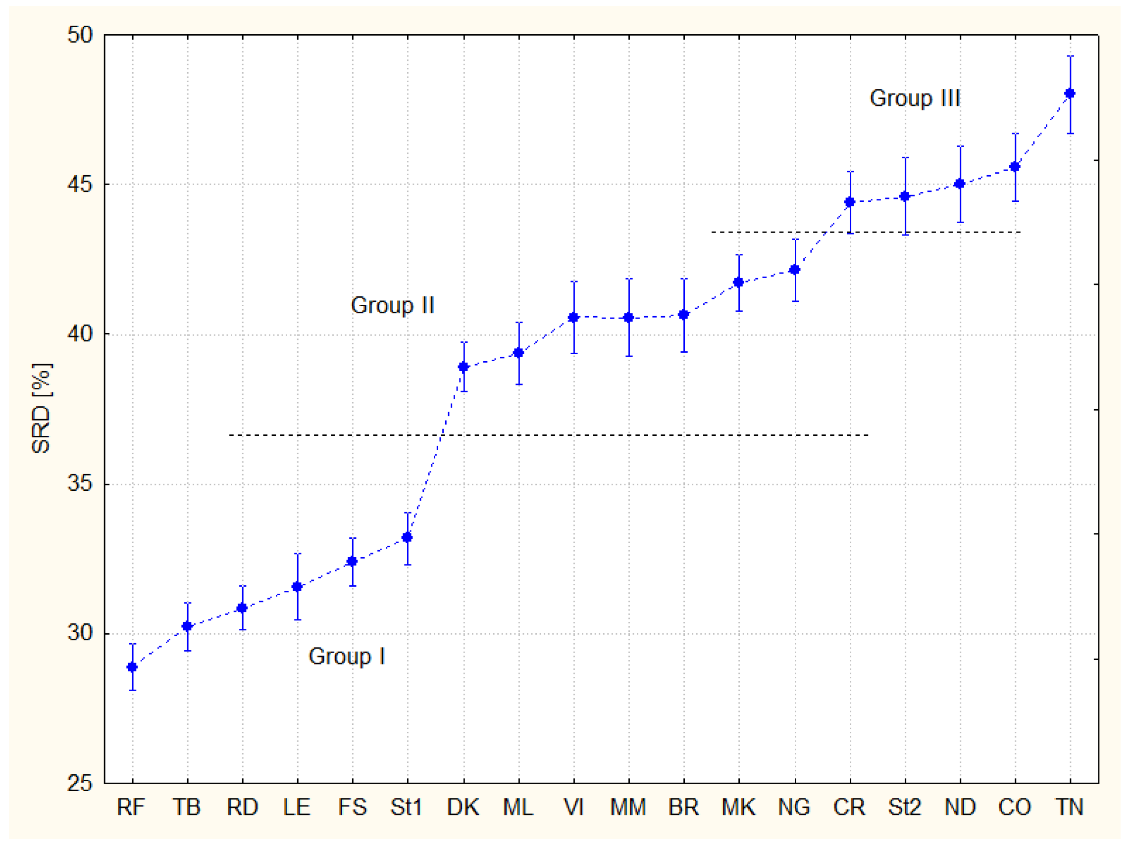
Figure 3 shows the characteristic grouping of experts. Post hoc tests suggest from six (Scheffé’s test) to nine (Tukey honestly significant difference test) overlapping groups, but three groups can be defined relatively easily (Figure 3): Group I (SRD < 35), Group II (37 < SRD < 43), and Group III (SRD > 43), I–group of recommendable experts, II–medium-moderate type experts, and III–not recommendable opinions.
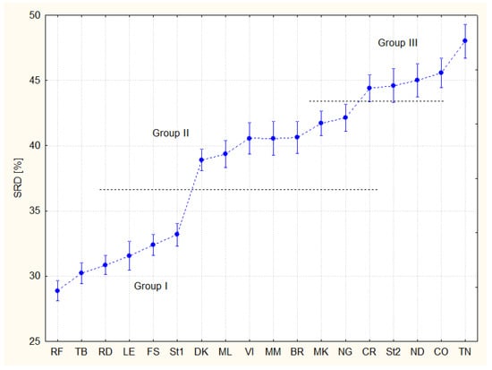
Figure 3.
Comparison of experts (F3, Sum of Ranking Differences, SRDs are scaled between 0 and 100). The coding options are amalgamated in F3. The error bars represent 95% confidence interval.
A slight difference can be observed if comparing the effect of rankings to the quality of experts (Figure 4): some experts seem to be better using GPA ranking while others do better at the re-ranking case.
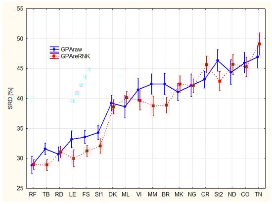
Figure 4.
Splitting of experts according to ranking options (F2*F3); Sum of Ranking Differences, SRDs are scaled between 0 and 100. The error bars represent 95% confidence interval.
In some cases (e.g., RD, DK, …) the two ranking options are indistinguishable. In other cases (e.g., FS, LE, St1, BR, MM, St2, …) the difference is significant, though not very large. The conclusion is obvious, the coding options should be tailored according to the preferences (taste) of the experts.
During the peer-review process, one of the unknown referees suggested to compare the obtained SRD rankings to other MCDM methods. After evaluating the existing literature, we decided to use the technique for order of preference by similarity to ideal solution (TOPSIS) method. Similar to the majority of MCDM methods, e.g., ELECTRE III, PROMETHEE methods etc., TOPSIS requires the definition of variable weights. Weights are meant to express the relative importance of the variables/criteria on the ranking of the objects/alternatives. There is no standard method for the definition of weights, rather, there are a set of approaches that could be followed [27,28]. Usually, two groups of weighting schemes are defined: so-called subjective and objective weights [29]. Subjective weights are usually defined by the decision makers (or users), while objective weights are defined by mathematical modelling. The authors of the present paper understand the difference between the two approaches; however, it has to be highlighted that the choice of models determining the objective weights are chosen by the decision makers, which are subjective. Therefore, it is always a trust issue to believe that weight definition methods have been chosen because they are “objective” or because they provided weights that are closer to the expectations of the decision maker/user. As a solution, we suggest choosing weight definition methods according to the data structure in order to reduce subjectivity.
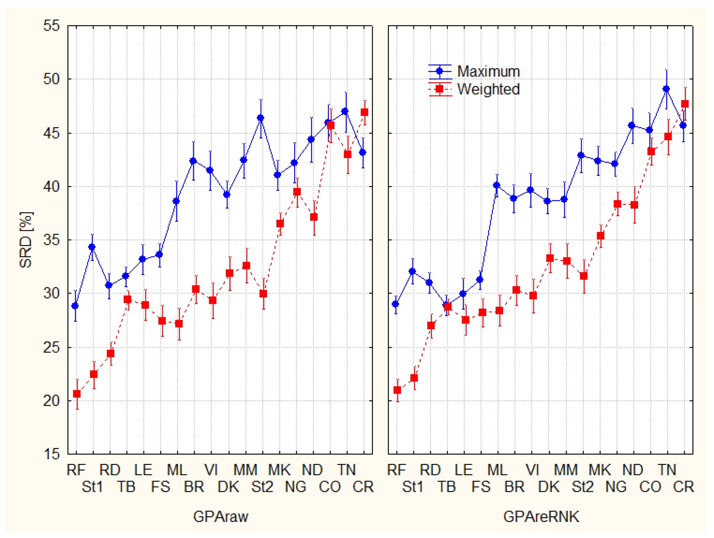
With these in mind, weights have been defined using the groupings presented by Figure 3. The first group of experts received the highest weights, while the third the lowest as follows: Group 1: 3/6, Group II: 2/6, and Group III 1/6. This weighting scheme was not only used for TOPSIS, but as a weighted SRD reference, as well. Figure 5 presents the decomposition of the two coding schemes with or without weighting. With the application of weights, smaller SRD values were obtained. Additionally, weights reduce (almost eliminate) the differences between the two coding schemes, as introduced by Figure 5. Out of these, the use of weights increases the number of experts in the second group (medium-moderate type experts), while decreasing the group of non-recommendable ones. For example, Figure 3 identifies five experts in the third group, while Figure 5 shows just three.

Figure 5.
Splitting of experts according to ranking options (F1*F2); Sum of Ranking Differences, SRDs are scaled between 0 and 100. The error bars represent 95% confidence interval. F1: GPAraw–original GPA coding, GPAreRank (recoding to full rank), F2: Maximum, Weighted.
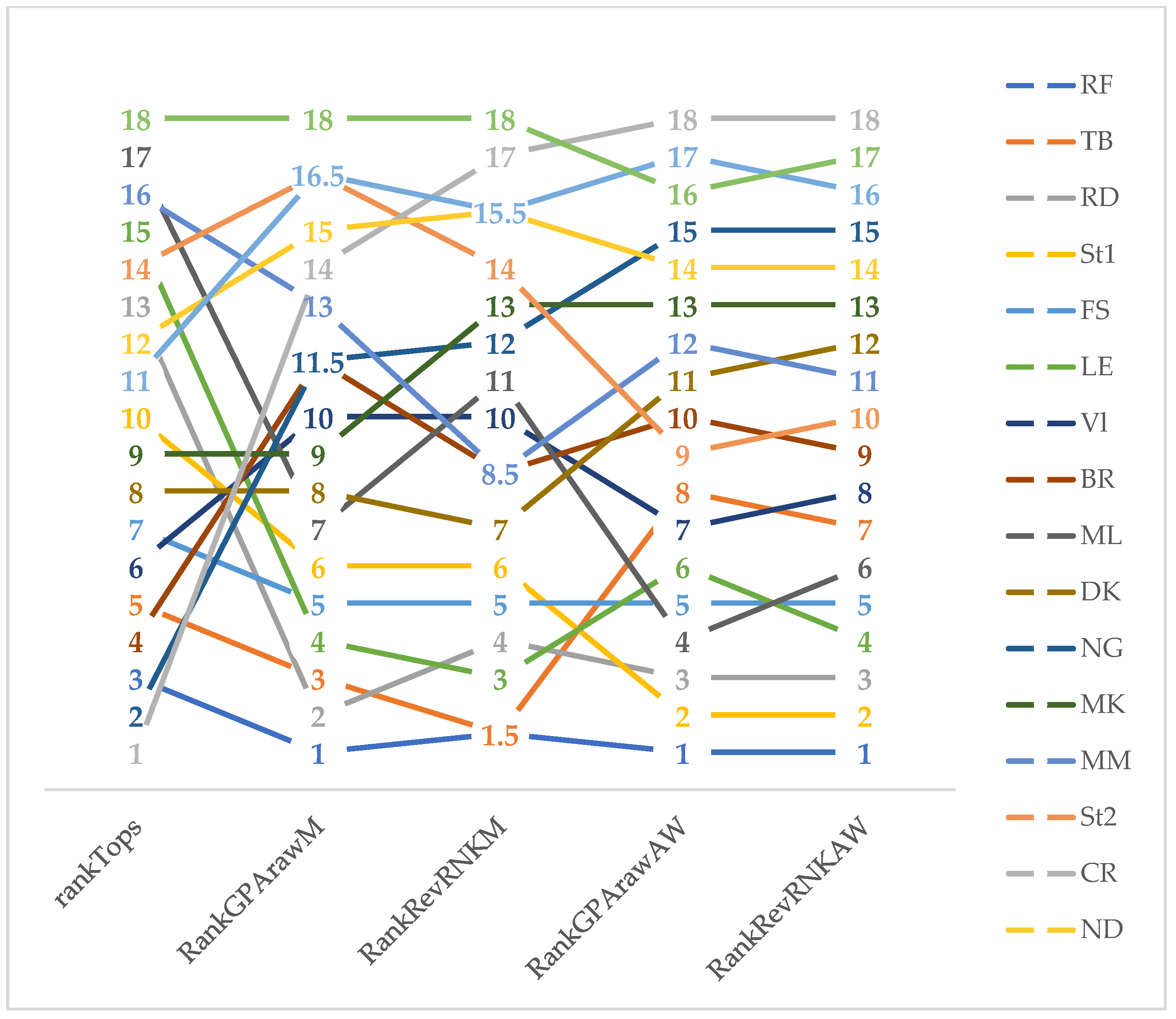
TOPSIS ranks have been compared to the SRD ranks in Figure 6. The first and last positions of experts are clearly found by almost all approaches, while the methods have lost consensus regarding the middle ranks. TOPSIS ranks differ the most, while it proved to be the most subjective due to the use of weights.
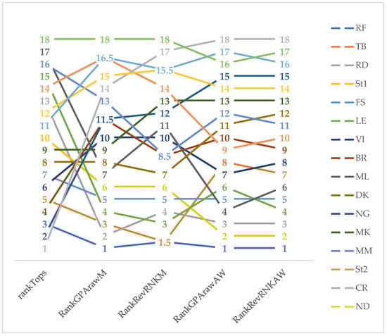
Figure 6.
Comparison of TOPSIS, original and weighted SRD rankings along with the two coding schemes. rankTops—TOPSIS ranks, RankGPArawM—SRD ranks of original GPA coding with maximum reference, RankRevRNKM—SRD ranks of recoding to full rank with maximum reference, RankGPArawW—SRD ranks of original GPA coding with weighted reference, RankRevRNKW—SRD ranks of recoding to full rank with weighted reference.
3.2. Evaluation of Teams
Multicriteria decision analysis can also be done on the transposed matrix, i.e., comparing the teams. Again, GPA coding and reranking the GPA codes were used (GPAcod and GPAreRNK, respectively) and two SRD rankings were carried out accordingly. Row-average was used as ideal ranking (reference) in SRD. It does not mean the ordering of teams is closer to the average teams; on the contrary, the ranking follows the experts’ averages. It is a simple assumption that none of the experts are perfect, some of them overestimate the teams’ performance, while others underestimate them. As the errors cancel each other out (at least partly), the average is the best choice (Figure 7).
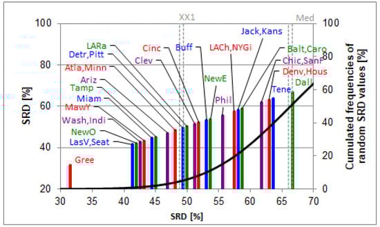
Figure 7.
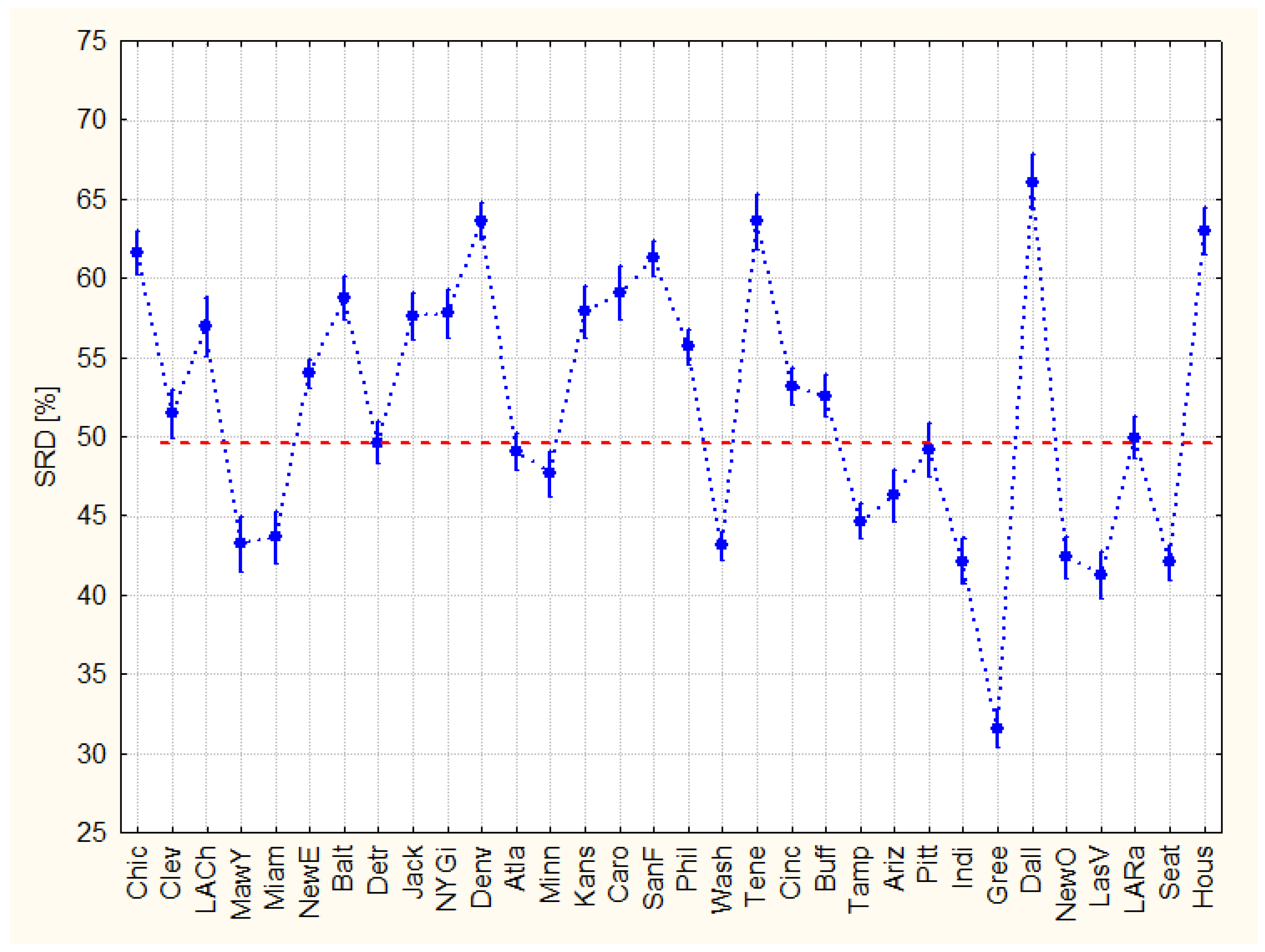
The SRD values (scaled between 0 and 100, blown up part) of the teams based on experts’ ratings determined by sum of ranking differences. Row-average values were used as the reference (benchmark) column. Scaled SRD values are plotted on the x axis and left y axis, right y axis shows the relative frequencies of random ranking distribution function: black curve. The probability ranges are also given as 5% (XX1), Median (Med), and 95% (XX19). Codes of the teams are listed in the data set section.
The teams right of the XX1 lines are indistinguishable from the random ranking. The Manhattan distances to the references (the SRD values) are real, independently whether the evaluation is seemingly random or not. The ordering shows a relative expectable performance. The distance from the first line (Gree) to zero shows the difficulty of evaluating teams, better experts, or their combination that we should be looking for.
The last validation step of the SRD values happened by a sevenfold cross-validation and by factorial ANOVA with Factor 1: resampling variant (two levels: contiguous sevenfold resampling–A, random resampling with replacement–B), Factor 2: coding (two levels: (1) GPA coding, (2) re-coding of GPA), and Factor 3: teams (32 levels).
The variances are homogenous according to the Levene’s test. Neither F1 nor F2 are significant, which is reassuring: we have not introduced any (other than random) information during coding and resampling. However, approximately half of the teams cannot be discriminated from random ranking. Similarly, the lack of points in the 0 < SRD < 30 range calls for a better grading system; more information should be involved in the evaluation (Figure 8).
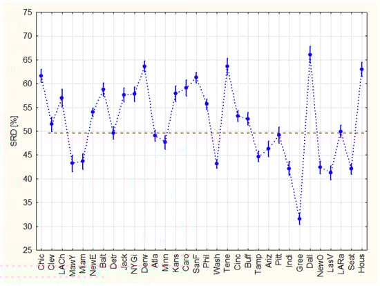
Figure 8.
Comparison of teams using sum of ranking differences (scaled between 1 and 100). The points of teams above the dotted red line are indistinguishable from random ranking.
Why the grading system of the NFL is “successful” (or at least used) then remains a question to be answered. If the random choice is so predominant, then any (even rubbish) evaluations are not necessarily distinguishable from serious approaches. In one sense, the highly random character in teams’ evaluation is reassuring as it reflects the main features of the issue and a perfect prediction would deteriorate all experts’ opinions, bookmaker’s activities and so on.
4. Discussion
There is still no clear consensus on which technique performs best; so, testing multicriteria decision making methods to discover the best one for the given situation is critical. Other studies sought to assess sports teams’ performance. Csató has demonstrated that multicriteria optimization produces more intuitive outcomes than lexicographic rankings. Based on an imperfect pairwise comparison matrix [30], an alternative ranking for the 2010 Chess Olympiad Open was introduced.
Dadelo and colleagues applied the technique of ordering performance by similarity to the ideal and worst solutions (TOPSIS) to ensure greater efficiency in basketball player and team qualification. More accurate prediction of sport performance, team composition, and optimization of the preparation process was realized, while taking into account the individualism of team players and encouraging their versatility, i.e., meeting the team’s overall physical fitness standards. The design and adaptation of mathematical systems for practical use considering the individuality and uniqueness of the athletes is crucial to optimize the training process of team players [31]. Although the proposed method showed promising results, it must be mentioned that a key point of TOPSIS models is the definition of the weights of the used the criteria (the weights are necessarily subjective and depend on the experts’ preferences). However, using experts’ opinions is a reliable option in cases where other methods are not available. Sum of ranking differences (SRD) gives a clear ranking and grouping of the variables instead, making it more robust to subjectivity.
As a solution to the weights issue, Chen and colleagues developed an evaluation model for selecting the best pitcher in the Chinese Professional Baseball League using the analytic hierarchy process (AHP) and TOPSIS models. The AHP was used to analyze the structure of the starting pitcher selection problem and to determine the weights of the criteria, while the TOPSIS method was used for the final ranking. It may not be realistic to develop a model that fits all decision makers and all decision situations [32]. In our case, the teams and experts were treated equally, as no weightings were applied.
Sinuany-Stern has also used the AHP method to rank football teams, using six criteria such as the performance of the previous season, the quality of the players or the team’s fans, etc. A pairwise comparison matrix was created for each criterion. The use of AHP seems to be appropriate for evaluating football teams, as the pairwise comparison of teams is natural [33]. One of the major advantages of SRD over AHP is that SRD is able to handle extremely large data sets. Therefore, there are almost no limitations regarding the number of criteria and/or decision options. Furthermore, in our case the input matrix was transposed, and the same data were used in a different perspective to evaluate not only the experts but also the teams themselves.
The technique for Order of Preference by Similarity to Ideal Solution (TOPSIS) was applied as an MCDM tool, with normalization and weighting. The weights of the criteria were calculated by an eight-step process using the fuzzy analytical hierarchy process (AHP). The TOPSIS, contrary to its name, does not rank the objectives to the similarity of the ideal solution as SRD does, but searches “the shortest geometric distance from the positive ideal solution (PIS) and the longest geometric distance from the negative ideal solution (NIS)” [34]. The same triangular fuzzy weighting was used in an AHP for the determination of the criteria of transport planners when establishing a set of park and ride system facilities [35].
In our case, TOPSIS weights were determined according to the data structure by the SRD grouping. However, we highlighted that the choice of weights is subjective in the case of “objective” weighting when it comes to choosing the method used for calculating the weights (there are a plethora of them). As TOPSIS ranks depend heavily on the weights, significant bias can be introduced if the weights are not properly chosen. This effect is even more expressed in cases where the impact of the teams is impossible to assess on the evaluation of the experts.
Kaczynska and colleagues compared chess players selected from the FIDE top 100 and ranked them according to their performance in different types of games and their age. It turned out that an unexpectedly high number of criteria should be taken into account to produce a reliable ranking. A ranking was created using the characteristic objects method (COMET). It is based on fuzzy logic and uses characteristic objects to evaluate alternatives, which guarantees immunity against the multiple ranking paradox. The COMET method is well suited for ranking problems in sports [36]. Fuzzy methods provide a solution for uncertainty and hesitancy during the decision process. In our SRD approach, the consensus method was used to eliminate the uncertainties and biases coming from the evaluations of the different experts.
Angulo and colleagues provided criteria for evaluating handball caps and used various soft computing methods to estimate their weights. They compared a fuzzy multicriteria decision making method, a metaheuristic optimization algorithm, and methods based on statistical and domain knowledge to evaluate goalkeepers’ actions during the game. The metaheuristic-based method outperformed other approaches in identifying and ranking the best handball goalkeeper. Furthermore, the fuzzy technique based on expert judgements has produced poor results in terms of selecting the best goalkeepers [37].
Fuzzy methods have also been used to evaluate the significance of the different performance criteria used later in an MCDM method. Nasiri and colleagues looked at the selection of sub-footballers for the transfer season using a fuzzy analytic network process (ANP) to weight the different field positions; then, the suitability of each player was computed via PROMETHEE II. The proposed method maximizes the total scores of the players to be purchased while keeping costs as low as possible [38].
In the case of basketball, Martínez and Martinez investigated the opinions of basketball stakeholders in several specific issues related to player evaluation. This macro-research involved players, coaches, agents, journalists, editors, bloggers, researchers, analysts, fans, and chairs. The current player evaluation systems are not sufficient to meet stakeholders’ expectations in terms of determining value, as they do not assess intangible values [39].
Hochbaum and Levin present a new paradigm using an optimization framework that addresses the main shortcomings of current models of group ranking. The framework provides a concrete performance measure for the quality of aggregate rankings based on deviations from the rankings of individual decision makers. The presented new model of the group ranking problem is based on intensity rankings, i.e., the degree of preference is quantified. The model allows for flexibility in decision protocols and can account for imprecise beliefs, incomplete confidence in individual rankings, and differences in the expertise of the raters [40].
In sports sciences, ranking problems can also arise when a set of alternatives characterized by variables and decisions are based on the pairwise comparisons of the alternatives (matches between players). The series of these pairwise comparisons give the tournaments, which can have different formats. Sziklai and colleagues compared these formats, such as knockout tournaments, multi-stage tournaments, and the Swiss-system, using Monte-Carlo simulations. Of all the tournament formats, the Swiss-system was found to be the most accurate, especially in terms of ranking all participants [41].
Three aspects were considered: pertinence, importance, and unambiguity [42] in developing an assessment of 11 play actions, decision-making, technical execution, and the final result were coded according to the observed adequacy. A panel of experts validated the instrument (camera).
A computer model was developed to calculate the probability that a pass reaches the target player without being intercepted by opponents in soccer. A comparison to expert ratings was fulfilled as a part of the model without using any MCDM methods [43].
Finally, the limitations of the SRD are gathered below. Although the SRD as an MCDM tool is entirely general and can be applied in highly diverse fields, there are some practical limitations:
- (i)
- Naturally, the results depend on the golden standard and the results will necessarily be changed if changing the benchmark. All variables (objectives) are used as a benchmark once and only once to resolve the benchmark ambiguity problem [15]. It was termed as COVAT (Comparisons with One Variable at a Time). A heatmap format was introduced to visualize the pairwise Manhattan distances (SRDs) [15].
- (ii)
- If the criteria are not conflicting, then the same ranking appears for each objective and no ordering takes place. However, it is a rare occasion, it happens only in the case of linearly dependent objectives.
- (iii)
- Different scales might lead to somewhat different ranking and grouping of the objectives. In such cases, more scaling options are advised to reach general conclusions; preferably, standardization, rank transformation, range scaling between 0 and 1, and normalization to unit length.
- (iv)
- The SRD computer codes do not allow weighting in their present version, though some decision makers would insist the favorable usage of preferred alternatives (criteria). This deficiency can easily be solved if we use a weighted standard as we have shown this possibility above cf. Figure 5 and the preceding corresponding text.
- (v)
- If the number of rows in the input matrix (the number of alternatives) is too small (say, below seven), then the probability of random ranking is enhanced though the most probable ordering outcome. If the number of rows surpasses 1400, then the fifth percentile of the randomization test provides a lower limit (conservative estimation). In practice, such a limitation is not a real one, as fully random ordering of 1400 items rarely happens, if at all.
5. Conclusions
A novel method, sum of ranking differences, was used, which provides a clear ranking and grouping of experts and teams to be compared alike. Thanks to its nonparametric nature, a diverse type of variables can be used to conduct the evaluations. The method has other potential fields of applications, starting from the comparison of players through the comparison of the performance of judges to the validation of other methods.
An important finding of the research is that rankings provide a better separation compared to GPA scores and that there is a significant deviation in experts’ opinions. The coding options should be tailored according to the preferences (taste) of the experts.
Around half of the teams cannot be distinguished from random ranking. Although the analysis identified Green Bay Packers as the team having the most promising draft, there are many other factors that can influence the teams’ performance during the season. A future direction therefore could be the continuous follow-up of the teams and expert opinions on the drafts to quantity the effect of the drafts on the performance of the team.
Author Contributions
Conceptualization, A.G. and K.H.; methodology, A.G. and K.H.; software, K.H.; validation, A.G. and K.H.; formal analysis, A.G. and K.H.; investigation, A.G., D.S. and K.H.; resources, A.G. and K.H.; data curation, A.G. and K.H.; writing—original draft preparation, A.G. and D.S.; writing—review and editing, K.H.; visualization, K.H., D.S.; supervision, K.H.; project administration, A.G. and K.H.; funding acquisition, A.G. All authors have read and agreed to the published version of the manuscript.
Funding
The research was supported by the Ministry of Innovation and Technology of Hungary from the National Research, Development and Innovation Fund (OTKA, contracts No K 134260 and FK 137577).
Institutional Review Board Statement
Not applicable.
Informed Consent Statement
Not applicable.
Data Availability Statement
The data presented in this study are available here: https://twitter.com/RNBWCV/status/1388864754450567169/photo/1 (accessed on 14 June 2022).
Acknowledgments
The work was also supported by the ÚNKP-21-5 New National Excellence Program of the Ministry for Innovation and Technology from the source of the National Research, Development and Innovation Fund. DSz thanks the support of the Doctoral School of Economic and Regional Sciences, Hungarian University of Agriculture and Life Sciences. AG thanks the support of the János Bolyai Research Scholarship of the Hungarian Academy of Sciences.
Conflicts of Interest
The authors declare no conflict of interest.
References
- Wolfson, J.; Addona, V.; Schmicker, R.H. The quarterback prediction problem: Forecasting the performance of college quarterbacks selected in the NFL draft. J. Quant. Anal. Sports 2011, 7, 12. [Google Scholar] [CrossRef] [Green Version]
- Mulholland, J.; Jensen, S.T. Predicting the draft and career success of tight ends in the National Football League. J. Quant. Anal. Sports 2014, 10, 381–396. [Google Scholar] [CrossRef] [Green Version]
- Becker, A.; Sun, X.A. An analytical approach for fantasy football draft and lineup management. J. Quant. Anal. Sports 2016, 12, 17–30. [Google Scholar] [CrossRef] [Green Version]
- Héberger, K.; Kollár-Hunek, K. Sum of ranking differences for method discrimination and its validation: Comparison of ranks with random numbers. J. Chemom. 2011, 25, 151–158. [Google Scholar] [CrossRef]
- Kollár-Hunek, K.; Héberger, K. Method and model comparison by sum of ranking differences in cases of repeated observations (ties). Chemom. Intell. Lab. Syst. 2013, 127, 139–146. [Google Scholar] [CrossRef]
- Rácz, A.; Bajusz, D.; Héberger, K. Consistency of QSAR models: Correct split of training and test sets, ranking of models and performance parameters. SAR QSAR Environ. Res. 2015, 26, 683–700. [Google Scholar] [CrossRef] [Green Version]
- Lourenço, J.M.; Lebensztajn, L. Post-Pareto Optimality Analysis with Sum of Ranking Differences. IEEE Trans. Magn. 2018, 54, 1–10. [Google Scholar] [CrossRef]
- Héberger, K.; Kollár-Hunek, K. Comparison of validation variants by sum of ranking differences and ANOVA. J. Chemom. 2019, 33, e3104. [Google Scholar] [CrossRef] [Green Version]
- Hastie, T.; Tibshirani, R.; Friedman, J.H. Cross-Validation. In Elements of Statistical Learning. Data Mining, Inference, Prediction; Springer: New York, NY, USA, 2009; Volume 764, p. 243. [Google Scholar]
- Gere, A.; Héberger, K.; Kovács, S. How to predict choice using eye-movements data? Food Res. Int. 2021, 143, 110309. [Google Scholar] [CrossRef]
- Gere, A.; Rácz, A.; Bajusz, D.; Héberger, K. Multicriteria decision making for evergreen problems in food science by sum of ranking differences. Food Chem. 2021, 344, 128617. [Google Scholar] [CrossRef]
- Héberger, K. Sum of ranking differences compares methods or models fairly. TrAC Trends Anal. Chem. 2010, 29, 101–109. [Google Scholar] [CrossRef]
- Nowik, W.; Héron, S.; Bonose, M.; Tchapla, A. Separation system suitability (3S): A new criterion of chromatogram classification in HPLC based on cross-evaluation of separation capacity/peak symmetry and its application to complex mixtures of anthraquinones. Analyst 2013, 138, 5801–5810. [Google Scholar] [CrossRef] [PubMed]
- Grisoni, F.; Cassotti, M.; Todeschini, R. Reshaped Sequential Replacement for variable selection in QSPR: Comparison with other reference methods. J. Chemom. 2014, 28, 249–259. [Google Scholar] [CrossRef]
- Andric, F.; Bajusz, D.; Racz, A.; Segan, S.; Heberger, K. Multivariate assessment of lipophilicity scales-computational and reversed phase thin-layer chromatographic indices. J. Pharm. Biomed. Anal. 2016, 127, 81–93. [Google Scholar] [CrossRef] [Green Version]
- Odovic, J.; Markovic, B.; Vladimirov, S.; Karljikovic-Rajic, K. Evaluation of Angiotensin-Converting Enzyme Inhibitor’s Absorption with Retention Data of Micellar Thin-Layer Chromatography and Suitable Molecular Descriptor. J. Chromatogr. Sci. 2015, 53, 1780–1785. [Google Scholar] [CrossRef] [Green Version]
- Gere, A.; Radványi, D.; Héberger, K. Which insect species can best be proposed for human consumption? Innov. Food Sci. Emerg. Technol. 2019, 52, 358–367. [Google Scholar] [CrossRef] [Green Version]
- Brownfield, B.; Kalivas, J.H. Consensus Outlier Detection Using Sum of Ranking Differences of Common and New Outlier Measures Without Tuning Parameter Selections. Anal. Chem. 2017, 89, 5087–5094. [Google Scholar] [CrossRef]
- Kovačević, S.; Karadžić, M.; Podunavac-Kuzmanović, S.; Jevrić, L. Binding affinity toward human prion protein of some anti-prion compounds—Assessment based on QSAR modeling, molecular docking and non-parametric ranking. Eur. J. Pharm. Sci. 2018, 111, 215–225. [Google Scholar] [CrossRef]
- Li, W.; Miao, W.; Cui, J.; Fang, C.; Su, S.; Li, H.; Hu, L.; Lu, Y.; Chen, G. Efficient Corrections for DFT Noncovalent Interactions Based on Ensemble Learning Models. J. Chem. Inf. Model. 2019, 59, 1849–1857. [Google Scholar] [CrossRef]
- Chen, X.; Xu, Y.; Meng, L.; Chen, X.; Yuan, L.; Cai, Q.; Shi, W.; Huang, G. Non-parametric partial least squares–discriminant analysis model based on sum of ranking difference algorithm for tea grade identification using electronic tongue data. Sens. Actuators B Chem. 2020, 311, 127924. [Google Scholar] [CrossRef]
- Miranda-Quintana, R.A.; Bajusz, D.; Rácz, A.; Héberger, K. Extended similarity indices: The benefits of comparing more than two objects simultaneously. Part 1: Theory and characteristics. J. Cheminform. 2021, 13, 32. [Google Scholar] [CrossRef] [PubMed]
- West, C. Statistics for Analysts Who Hate Statistics, Part VII: Sum of Ranking Differences (SRD). LC-GC N. Am. 2018, 36, 882–885. [Google Scholar]
- Herrera-Viedma, E.; Herrera, F.; Chiclana, F. A consensus model for multiperson decision making with different preference structures. IEEE Trans. Syst. Man Cybern. Part A Syst. Hum. 2002, 32, 394–402. [Google Scholar] [CrossRef]
- Boccard, J.; Rutledge, D.N. A consensus orthogonal partial least squares discriminant analysis (OPLS-DA) strategy for multiblock Omics data fusion. Anal. Chim. Acta 2013, 769, 30–39. [Google Scholar] [CrossRef] [PubMed]
- Mansouri, K.; Ringsted, T.; Ballabio, D.; Todeschini, R.; Consonni, V. Quantitative Structure–Activity Relationship Models for Ready Biodegradability of Chemicals. J. Chem. Inf. Model. 2013, 53, 867–878. [Google Scholar] [CrossRef] [PubMed]
- Olson, D.L. Comparison of weights in TOPSIS models. Math. Comput. Model. 2004, 40, 721–727. [Google Scholar] [CrossRef]
- Vavrek, R. Evaluation of the Impact of Selected Weighting Methods on the Results of the TOPSIS Technique. Int. J. Inf. Technol. Decis. Mak. 2019, 18, 1821–1843. [Google Scholar] [CrossRef]
- Wang, T.-C.; Lee, H.-D. Developing a fuzzy TOPSIS approach based on subjective weights and objective weights. Expert Syst. Appl. 2009, 36, 8980–8985. [Google Scholar] [CrossRef]
- Csató, L. Ranking by pairwise comparisons for Swiss-system tournaments. Cent. Eur. J. Oper. Res. 2013, 21, 783–803. [Google Scholar] [CrossRef] [Green Version]
- Dadelo, S.; Turskis, Z.; Zavadskas, E.K.; Dadeliene, R. Multi-criteria assessment and ranking system of sport team formation based on objective-measured values of criteria set. Expert Syst. Appl. 2014, 41, 6106–6113. [Google Scholar] [CrossRef]
- Chen, C.; Lin, M.; Lee, Y.; Chen, T.; Huang, C. Selection best starting pitcher of the Chinese professional baseball league in 2010 using AHP and TOPSIS methods. In Frontiers in Computer Education, Advances in Intelligent and Soft Computing; Sambath, S., Zhu, E., Eds.; Springer: Berlin/Heidelberg, Germany, 2012; Volume 133, pp. 643–649. ISBN 9783642275517. [Google Scholar]
- Sinuany-Stern, Z. Ranking of sports teams via the ahp. J. Oper. Res. Soc. 1988, 39, 661–667. [Google Scholar] [CrossRef]
- Wang, C.N.; Tsai, H.T.; Nguyen, V.T.; Nguyen, V.T.; Huang, Y.F. A hybrid fuzzy analytic hierarchy process and the technique for order of preference by similarity to ideal solution supplier evaluation and selection in the food processing industry. Symmetry 2020, 12, 211. [Google Scholar] [CrossRef] [Green Version]
- Ortega, J.; Tóth, J.; Moslem, S.; Péter, T.; Duleba, S. An Integrated Approach of Analytic Hierarchy Process and Triangular Fuzzy Sets for Analyzing the Park-and-Ride Facility Location Problem. Symmetry 2020, 12, 1225. [Google Scholar] [CrossRef]
- Kaczynska, A.; Kołodziejczyk, J.; Sałabun, W. A new multi-criteria model for ranking chess players. Procedia Comput. Sci. 2021, 192, 4290–4299. [Google Scholar] [CrossRef]
- Angulo, E.; Romero, F.P.; López-Gómez, J.A. A comparison of different soft-computing techniques for the evaluation of handball goalkeepers. Soft Comput. 2021, 26, 3045–3058. [Google Scholar] [CrossRef]
- Nasiri, M.M.; Ranjbar, M.; Tavana, M.; Santos Arteaga, F.J.; Yazdanparast, R. A novel hybrid method for selecting soccer players during the transfer season. Expert Syst. 2019, 36, e12342. [Google Scholar] [CrossRef] [Green Version]
- Martínez, J.A.; Martínez, L. A stakeholder assessment of basketball player evaluation metrics. J. Hum. Sport Exerc. 2011, 6, 153–183. [Google Scholar] [CrossRef] [Green Version]
- Hochbaum, D.S.; Levin, A. Methodologies and algorithms for group-rankings decision. Manag. Sci. 2006, 52, 1394–1408. [Google Scholar] [CrossRef]
- Sziklai, B.R.; Biró, P.; Csató, L. The efficacy of tournament designs. Comput. Oper. Res. 2022, 144, 105821. [Google Scholar] [CrossRef]
- García-Ceberino, J.M.; Antúnez, A.; Ibáñez, S.J.; Feu, S. Design and Validation of the Instrument for the Measurement of Learning and Performance in Football. Int. J. Environ. Res. Public Health 2020, 17, 4629. [Google Scholar] [CrossRef]
- Dick, U.; Link, D.; Brefeld, U. Who can receive the pass? A computational model for quantifying availability in soccer. Data Min. Knowl. Discov. 2022, 36, 987–1014. [Google Scholar] [CrossRef]

Publisher’s Note: MDPI stays neutral with regard to jurisdictional claims in published maps and institutional affiliations. |
© 2022 by the authors. Licensee MDPI, Basel, Switzerland. This article is an open access article distributed under the terms and conditions of the Creative Commons Attribution (CC BY) license (https://creativecommons.org/licenses/by/4.0/).