Article

Estimation of Atmospheric Gusts Using Integrated On-Board Systems of a Jet Transport Airplane—Flight Simulations

1
Doctoral School of Engineering and Technical Sciences, Rzeszow University of Technology, al. Powst. Warszawy 8, 35-959 Rzeszów, Poland
2
Department of Avionics and Control Systems, Faculty of Mechanical Engineering and Aeronautics, Rzeszow University of Technology, al. Powst. Warszawy 8, 35-959 Rzeszów, Poland
*
Authors to whom correspondence should be addressed.
Appl. Sci. 2022, 12(13), 6349; https://doi.org/10.3390/app12136349
Submission received: 14 May 2022 / Revised: 13 June 2022 / Accepted: 20 June 2022 / Published: 22 June 2022
(This article belongs to the Section Aerospace Science and Engineering)

Abstract

:
Currently, quite accurate measurements of atmospheric gusts are carried out by airport systems only in the vicinity of the runways. There is a still open issue of availability of information about real wind gusts at cruising altitudes and during approach at a considerable distance from the airfield. Standard on-board systems of a jet transport airplane provide some information which is desirable to have knowledge of how flight parameters reflect real gust parameters and their impact on the aircraft dynamics. The paper proposes an algorithm for headwind gust magnitude estimation in relation to aircraft response. The analysed estimation algorithms assume the use of data available from the existing on-board systems only without the employment of any extra sensors or ground and satellite systems. In this way, many problems caused by different structures, configurations, and ways of installation of additional sensors and structural changes are rejected. The algorithms use the classical method for estimation of wind parameters as well as a linear longitudinal model of aircraft dynamics, taking into account the influence of wind gusts. Data fusion was realised with the use of three filtration methods. Results were evaluated to select the most accurate method of the estimation. Test data were obtained from advanced flight simulation. The experimental scenario considered a flight of a passenger twin-engine jet airplane through a layer of programmed gusts. The results of the flight simulations allowed us to determine the accuracy of the proposed gust estimation algorithms in reference to the ideal wind-speed data analysis obtained directly from the simulation environment (with the accuracy of the simulation process). The use of the proposed gust estimation algorithms may provide more accurate signal for integrated on-board systems, especially for wind shear detection and sped-up response time of flight control systems, protecting aircrafts against the adverse impact of encountered wind shear or gusts, e.g., auto-thrust or auto-throttle systems. The dedicated algorithm presented in the paper may increase the safety level of take-off and approach phases in gusty conditions and also during significant changes in wind speed at cruising altitudes in the case of crossing the area of jet stream occurrence.

1. Introduction

Heterogeneous wind fields such as turbulence or wind gusts cause changes in local aerodynamic forces and momentums, affecting aircraft structure and which can be a causative factor of air operation safety. According to the International Civil Aviation Organisation, the change in headwind of 15 kt (7.6 m/s) or more at an altitude below 1600 ft (or 500 m) at a 3 nautical mile (5000 m) radius from the runway threshold is classified as significant low-level wind shear (ICAO, ang. International Civil Aviation Organization, 2005) [1]. Wind shear happening on a meteorological microscale (effective range less than few nautical miles) is characteristic to airfields located on islands or in mountainous areas, affecting the safety of take-off and approach phases during which the aircraft operates close to critical angles of attack [2,3,4,5]. Sudden changes in both direction and wind speed are also results of meteorological phenomena occurring on a synoptical scale (squall lines, atmospheric fronts, and inversions). The danger can be posed by the phenomenon known as the clear air turbulence (CAT) [6], appearing in the close proximity of jet streams in a clear atmosphere. They emerge as a result of differences in wind speed at various altitudes, mainly flight levels which correspond with a narrow spectrum of available airspeeds—the coffin corner. In such a scenario, the stall speed is in proximity to the critical Mach speed for airliners.
The wind shear prognosis is challenging and not always possible to be accomplished due to the local and time-limited characteristic of this phenomenon. The dynamic development of civil aviation has brought the development of warning systems protecting against wind shear. Because of high maintenance costs, advanced airfield systems detecting wind shear such as the low level wind shear alert system (LLWAS) and terminal doppler weather radar (TDWR or SODAR) [7] are being used only by the minority of the most important airports around the world. Most airports accomplish standard measurements of wind direction and speed as well as gusts with the use of anemometers localised in the adequate runway area. An accurate measurement is able to be obtained during the last seconds of approach and on flare and touchdown. Because of that, for a majority of flight phases and considering automatic steering systems, the most important thing is the accuracy of measurement accomplished by the on-board systems. The on-board wind shear warning systems “WSWS” can be divided into reactive wind shear systems “RWS” using direct measurements of flight parameters and predictive wind shear systems “PWS”, working on the principle of prediction of wind shear preceding the aircraft by 10–40 s.
In the last years, main jet aircraft producers have been focused on the development of PWS. In one of the latest constructions—Boeing 787—the gust suppression system was used. During the automatic phase of flight, it utilizes the symmetric deflection of the flaperons and elevators to alleviate gust acceleration. Lateral gust suppression improves ride quality by automatic application of discrete yaw commands in response to lateral gusts and turbulence [8]. The research on widening the functionality of existing systems is based upon improvement of the ability of foreseeing future loads as a means of supplying updated data for an anticipated load. The use of the LIDAR [9,10] sensor is considered as an on-board solution. It works on the principle of laser beams instead of microwaves, allowing one to obtain data about radial wind velocity at various distances. The compensation of wind gusts is accomplished through a change in aerodynamic loads. Pitching the aircraft is the most effective way of achieving the above-mentioned goal. Another way is through the use of steering surfaces, e.g., ailerons and spoilers, or even through direct lift control DLC [9]. The concept of minimising the load of gusts with the use of the Doppler LIDAR [7] sensor is based on the measurement of atmospheric disturbances before they reach the aircraft wings and exert further loads on construction. It is worth noticing that the above-mentioned warning systems provide the information about dangerous phenomena to aircrews so that adequate escape and avoiding manoeuvres can be executed. The analysis of the functioning of the automatic control systems as well as aircrew opinions suggests that a more accurate gust measurement system in challenging conditions would be useful, but in conditions not yet precluding the continuation of approach or exercising wind shear escape manoeuvres [11].
One of means of protecting aircraft against the adverse and severe impact of gusts are procedures described in the aircraft flight manual. Procedures often assume during flight at a cruising altitude that the auto-throttle system needs to be reloaded or disabled to prevent exceeding the maximum allowed speed regardless of previously set limitations [12]. Hence, during the gusts, both precision and reaction time are insufficient. Thus, a question is if it is possible that in gusty conditions, the autopilot might get disconnected, although the system remains stabilized on the correct glide path. Despite the fact that auto-throttle is not required for flights in reduced vertical separation minima (RVSM) airspace or for automatic landing used in ILS CAT II, the sudden disconnection of the system is an additional element of surprise, which contributes to the safety of operation.
Based on analysis of on-board measurement systems of the aircraft and taking into consideration increasing reactive capabilities of direct measurements, it was observed that the auto-throttle input signal, which refers to the airspeed, comes from the air data inertial reference unit (ADIRU) left and right. Every ADIRU consists of two subsystems: air data reference (ADR) and inertial reference (IR) [12,13]. The IR subsystem is based on three laser gyroscopes and three accelerometers, providing the data about: attitude, heading, present position, and acceleration. Airspeed information comes from the ADR and is based on pressure measurements characterised by a relatively long delay. The commonly used techniques for on-board estimation of wind speed and direction result from the analysis of TAS and GS velocity vectors [3,14]. In order to reduce delays in the wind parameter estimation process and exclude the influence of airplane control on the obtained result, inertial measurements and flight dynamics are also taken into account [15,16,17]. A gust of the same intensity acting on a small airplane or an unmanned aerial vehicle (UAV) [18,19,20] has a different impact on its accelerations than acting on an airplane which weigh a dozen tons [21]. Massive airplanes’ responses are slower and more delayed in time. In our work, for the purpose of estimating headwind gusts, it was decided to take into account the complex reaction of the aircraft in the longitudinal mode of motion. The main assumption of the presented method is a quick change of the pitch rate and pitch rate acceleration resulting from the headwind gust. Unfortunately, these parameters are also extremely affected by the operation of the control system (thrust change, and especially the elevator deflection). However, taking into account the model of the longitudinal motion of the aircraft in the estimation process allows for the compensation of this effect. The original contribution of this work is the integration of dependencies resulting from the linear mathematical model of longitudinal motion of the aircraft (taking into account the impact of headwind and vertical gusts on aircraft dynamics) with the classical method estimating wind parameters.
The work was carried out assuming the practical availability of all signals required for estimation. With the integration of the data already available from on-board systems such as ADIRU and Global Positioning System (GPS), an algorithm was developed. An original element of the work is also the integration of the simulation environment enabling the generation and recording of wind gust parameters (ideal) and their estimation using data provided by standard on-board instruments. The simulations were carried out using a complex non-linear model of aircraft dynamics in the X-Plane 11 environment, while the estimation algorithm uses a simplified linear model practical for efficient computations.

2. Theoretical Background

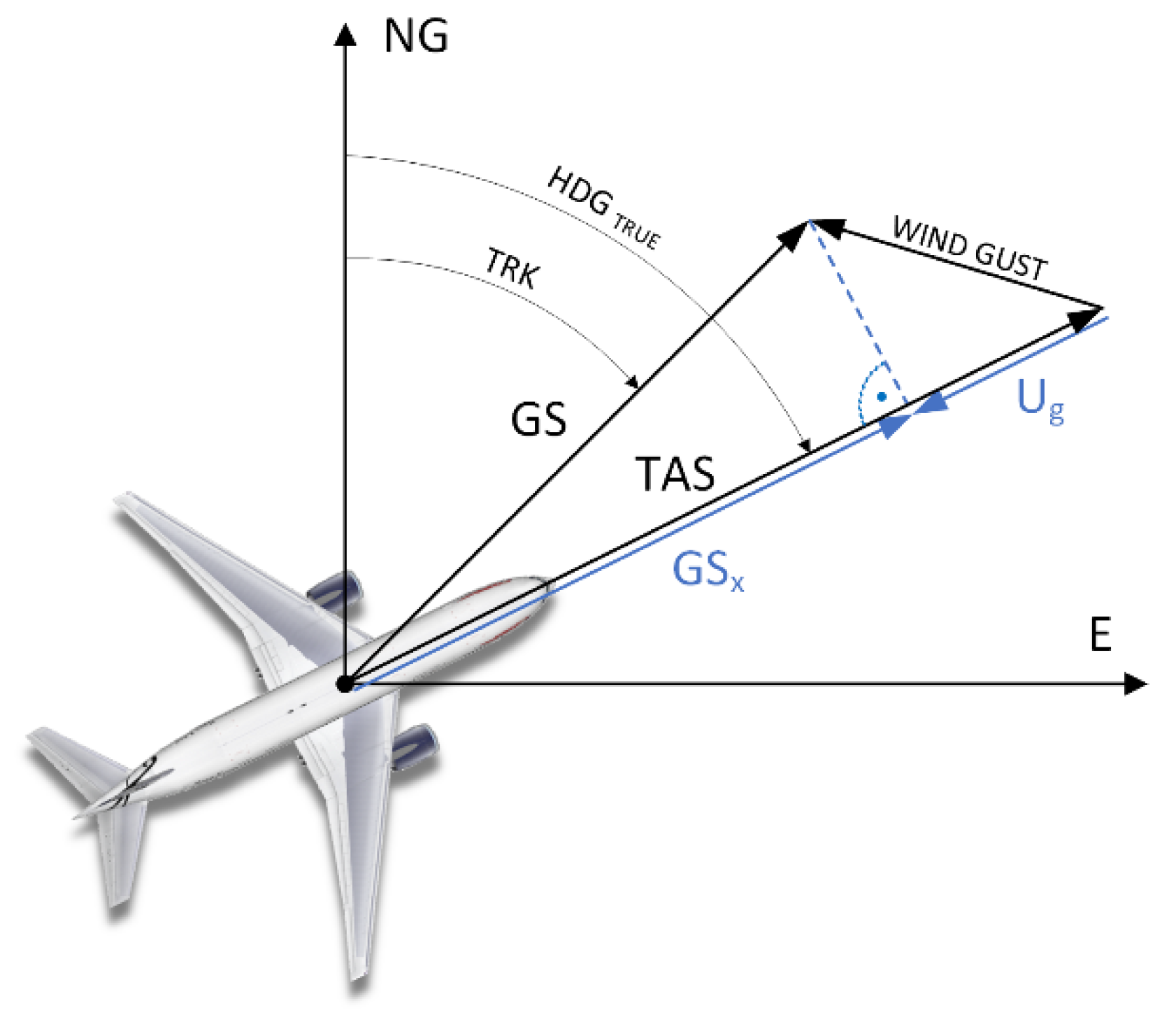
2.1. Analysis of the Possibility of Head-on Gusts Estimation

The wind gust speed component in the longitudinal axis of the airplane (Ug) can be estimated from the vector difference in measured true airspeed (TAS) and the ground speed component GSx, measured on the x-axis of the airplane (1). Positive sign of U g indicates the wind blowing into the nose of the plane—headwind (Figure 1).
U g = G S x T A S
Using the dependencies presented in Figure 1 and knowing the true heading (HGDtrue) and track (TRK) angles, apart from the Ug component, it is also possible to estimate the direction and total speed of wind as well as the lateral component of wind gust. In this paper, this issue was omitted by focusing on the wind component occurring in the longitudinal axis of the aircraft. This parameter is crucial for flight safety due to the possibility of an unexpected stall.
This estimation works well for slow changes in wind speed and direction. Equation (1) can be easily derived from the general form presented in the works [1,22,23,24,25]. The TAS measurement is carried out on-board the transport aircraft directly with the use of the systems air data computer (ADC) or air data inertial reference system (ADIRU/ADIRS). Determination of the component G S x requires measurement of G S and true track (TRK) as well as measuring the airplane’s true heading (HDGtrue). These data can be obtained from the satellite navigation system (GNSS) and/or the ADIRU/ADIRS. Measurement of TAS and G S x is characterised by considerable inertia and time constants of up to a few seconds (depending on the structure of the system, sensors, and algorithms used). Therefore, in the following part of the article, the estimation of Ug is identified with the low-frequency component of headwind estimation (Ug-lo), according to the identity (2).
U g - l o U g
Dangerous gusts of wind are usually characterised by immediate changes, and for their estimation, it is necessary to refer to the fast-changing state variables. The mathematical model of the airplane may be the equations of longitudinal and lateral motion [26]. They are usually two systems of linearised ordinary differential Equations (3) and (4).
d d t X l o n = A l o n · X l o n + B l o n · U l o n + C l o n · Z l o n
d d t X l a t = A l a t · X l a t + B l a t · U l a t + C l a t · Z l a t
State variables are defined as (for longitudinal and lateral motion, respectively):
Xlon = (u, w, q, υ)T   Xlat = (v, p, r, φ)T
Control vectors (U) and disturbances (Z) are instead:
Ulon = (δH, δT)T   Zlon = (wg, ug)T    Ulat = (δL, δK)T   Zlat = (vg)T
The presented mathematical model of the aircraft was constructed based on the theory of flight mechanics. Matrices of coefficients (7) and (8) appearing in the equations of longitudinal motion (3) and lateral motion (4) contain the corresponding aerodynamic derivatives.
A lon = [ X u X w 0 g cos Θ 0 Z u Z w U 0 g sin Θ 0 M u ¯ M w ¯ M q ¯ 0 0 0 1 0 ]   B lon = [ X δ H X δ T Z δ H Z δ T M δ H ¯ M δ T ¯ 0 0 ]   C lon = [ X w X u Z w Z u M w ¯ M u ¯ 0 0 ]
A l a t = [ Y V Y p Y r U 0 g cos Θ 0 L v L p L r 0 N v N p N r 0 0 1 t g Θ 0 0 ]   B lat = [ Y δ L Y δ K L δ L L δ K N δ L N δ K 0 0 ]   C lat = [ Y v g L v g N v g 0 ]
Increase in the gust value in the longitudinal axis of the airplane ug occurs in the equation for the longitudinal motion of the airplane (3) in the disturbance vector Zlon (6). Substituting matrices Alon, Blon, and Clon and vectors Xlon, Ulon, and Zlon to Equation (3), we obtain four equations. A third of them can be directly written as a dependence (9).
q ˙ = M u ¯ · ( u u g ) + M w ¯ · ( w w g ) + M q ¯ · q + M δ H · δ H + M δ T · δ T
It should be emphasized that q ˙ , u, ug, w, wg, q, δH, and δT represent increments in value and are not absolute values. This is because Equations (3) and (4) represent an incremental model. This property was taken into account in the process of modelling the estimation system. Assuming a constant descent rate W (increment of this parameter is zero, so we can assume w = 0), no vertical gusts (wg = 0), and constant thrust (δT = 0), we can reduce the dependency (9) to the form (10):
q ˙ = M u ¯ · ( u u g ) + M q ¯ · q + M δ H · δ H
By transforming the dependency (10) with respect to ug, we obtain Equation (11):
u g = M q ¯ M u ¯ · q ˙ 1 M u ¯ · q + M δ H M u ¯ · δ H + 1 M u ¯ · u
By introducing gain factors k1, k2, k3, and k4, Equation (11) takes the form (12).
u g = k 1 · q ˙ k 2 · q + k 3 · δ H + k 4 · u
In the following part of the article, the estimation of ug is identified with high frequency estimation of headwind gust (ug-hi), according to the identity (13).
u g - h i u g

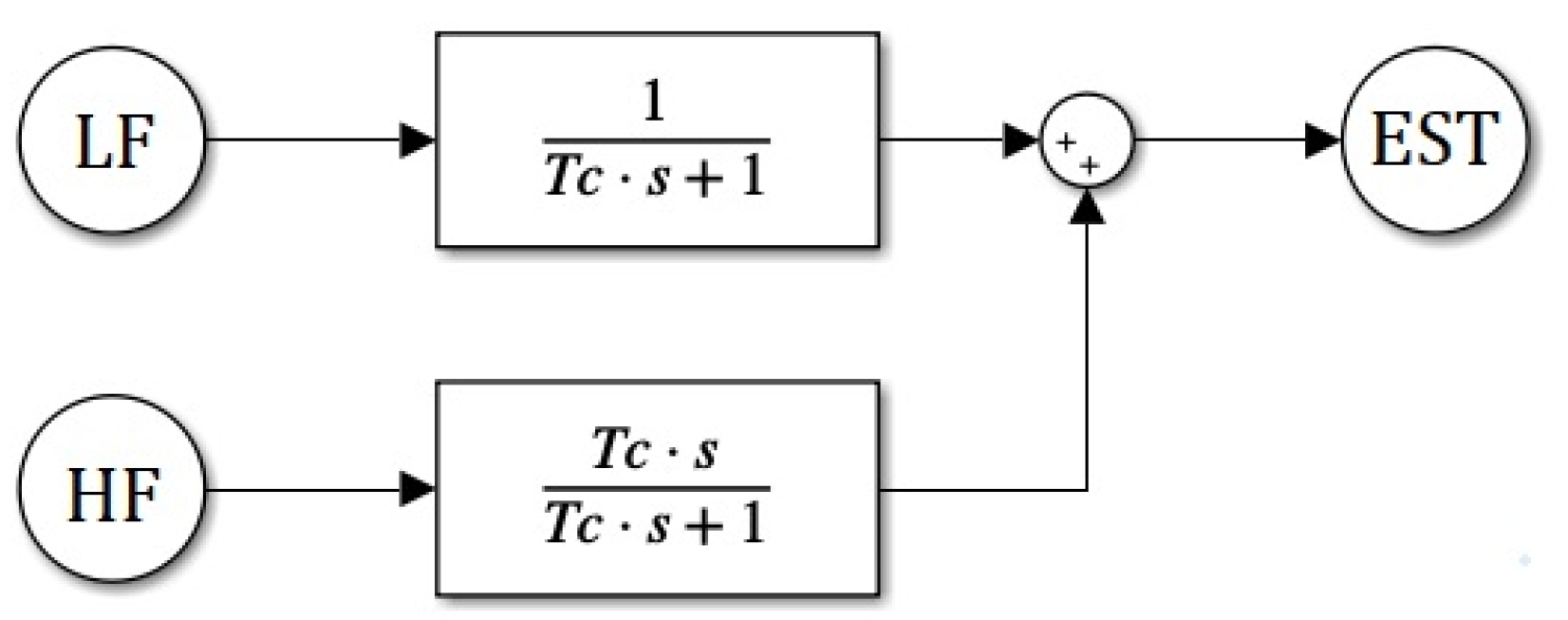
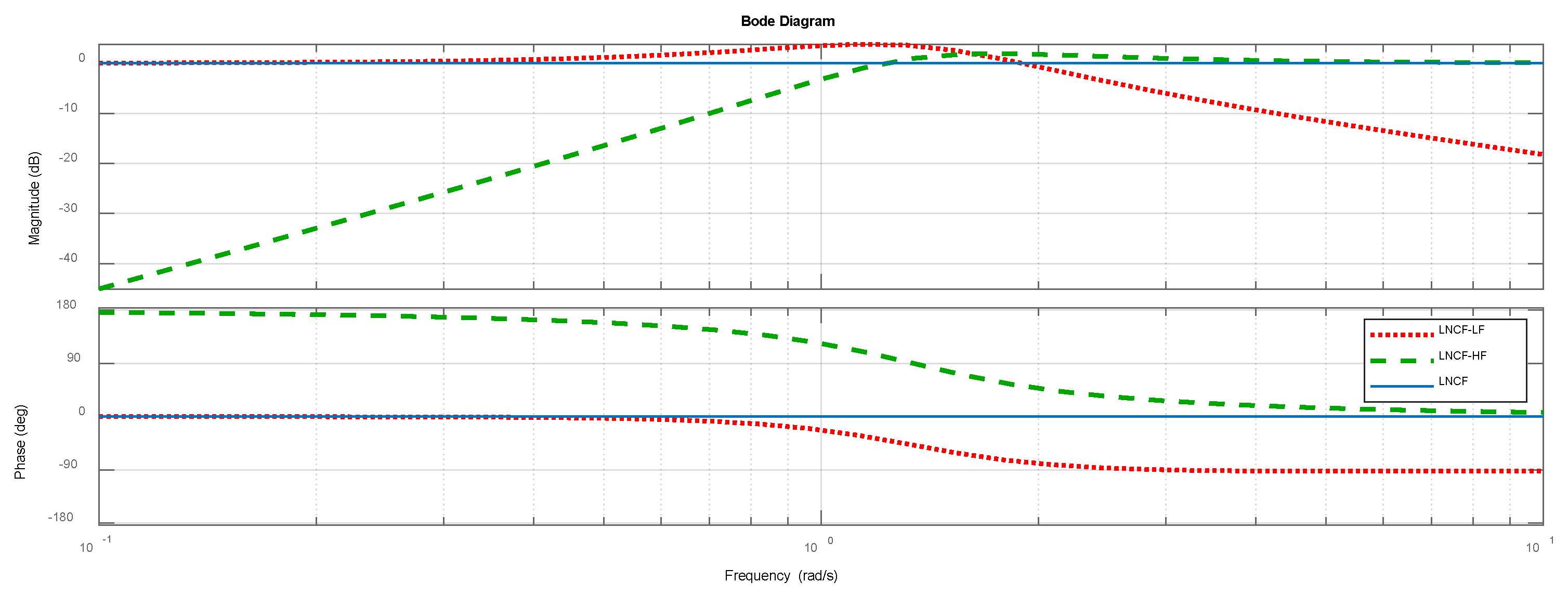
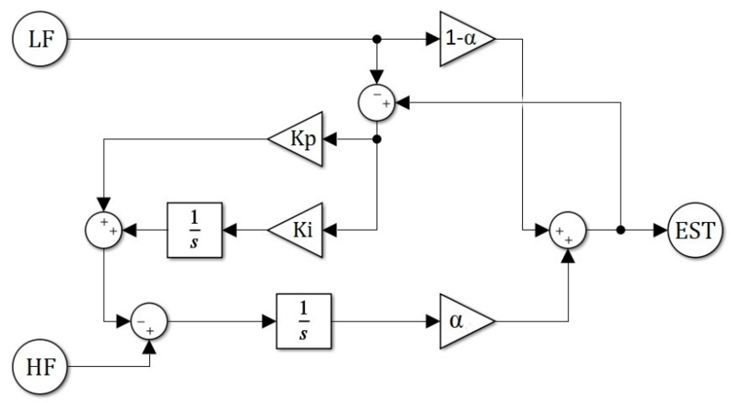
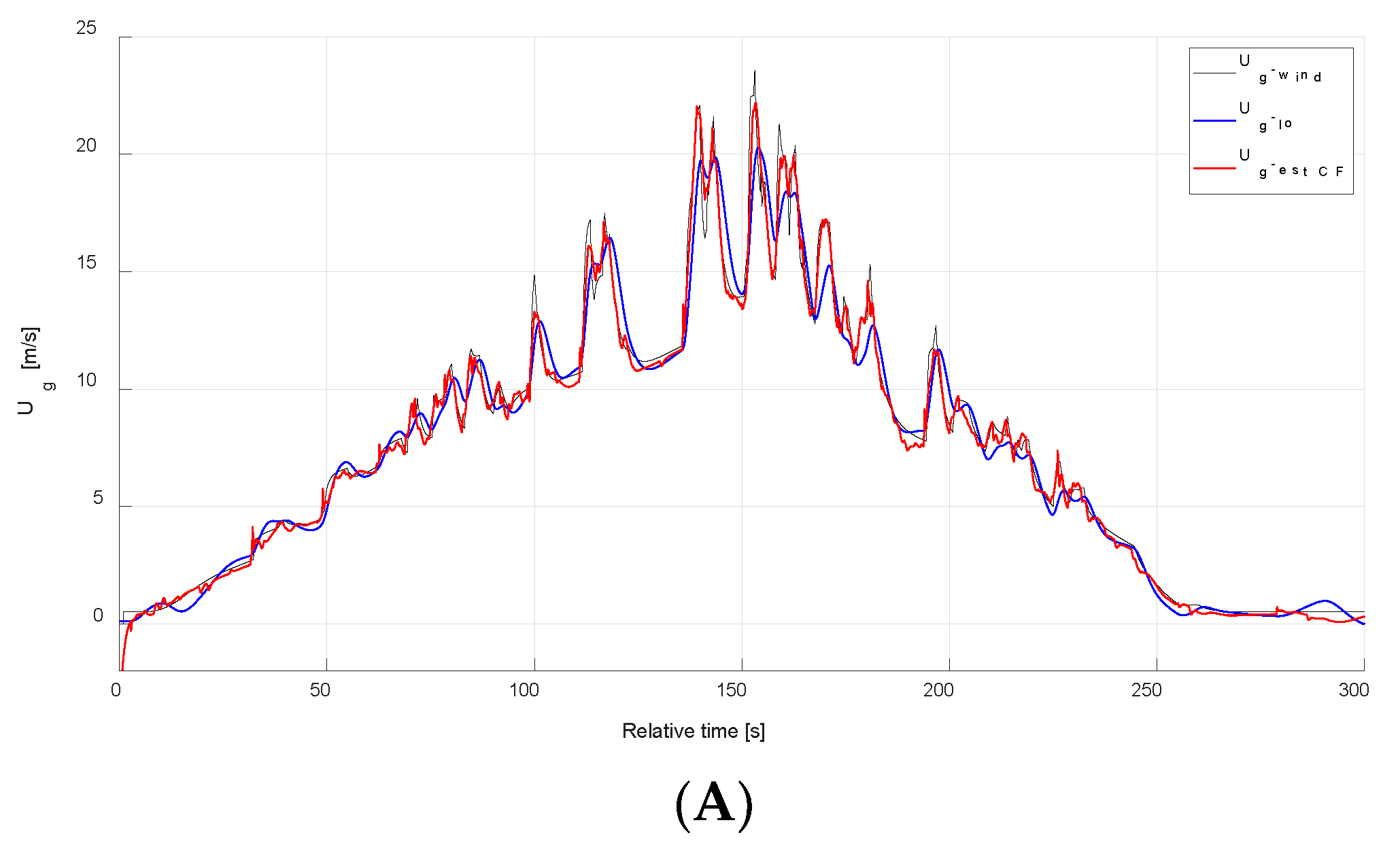
2.2. The Use of a Complementary Filter for Estimation of Headwind Gusts

The research hypothesis of this work assumes that the proposed method of estimating the value of the headwind component defined by Equation (1) and the temporary value of its change (gust) defined by Equation (12) can be used complementarily. Equation (1) can be used to determine the total value of the wind speed (headwind component). Due to the nature of the measured speeds GS and TAS (considerable delay of measurements), there are hard limitations related to the quick and precise detection of gusts. Equation (12), on the other hand, may be used to estimate the value of short-term changes in the headwind component, but it cannot be used to determine its absolute value. A natural solution in this situation seems to be the use of a complementary filtration system. The complementary filter (CF) is a computationally inexpensive and relatively efficient data fusion technique that consists of a low-pass and a high-pass filter [27]. The general structure of CF (Figure 2) consists of low- and high-frequency inputs of the composite signal.
The complementary filter transfer function is represented by Equation (14). The amplitude of linear CF is unity (0 dB magnitude) over the complete frequency range. The phase shift is also linear and equals 0 deg (Figure 3).
E S T = 1 T c · s + 1 · L F + T c · s T c · s + 1 · H F
  • LF—low-frequency signal,
  • HF—high-frequency signal,
  • EST—output of CF.
On the basis of dependencies (1), (2), (12)–(14), the complete law of headwind estimation (including temporary gusts) can be formulated as (15), and finally, as Equation (16).
U g - e s t _ C F = 1 T c · s + 1 · U g - l o + T c · s T c · s + 1 · u g - h i
U g - e s t _ C F = 1 T c · s + 1 · ( G S x T A S ) + T c · s T c · s + 1 · ( k 1 · q ˙ k 2 · q + k 3 · δ H + k 4 · u )

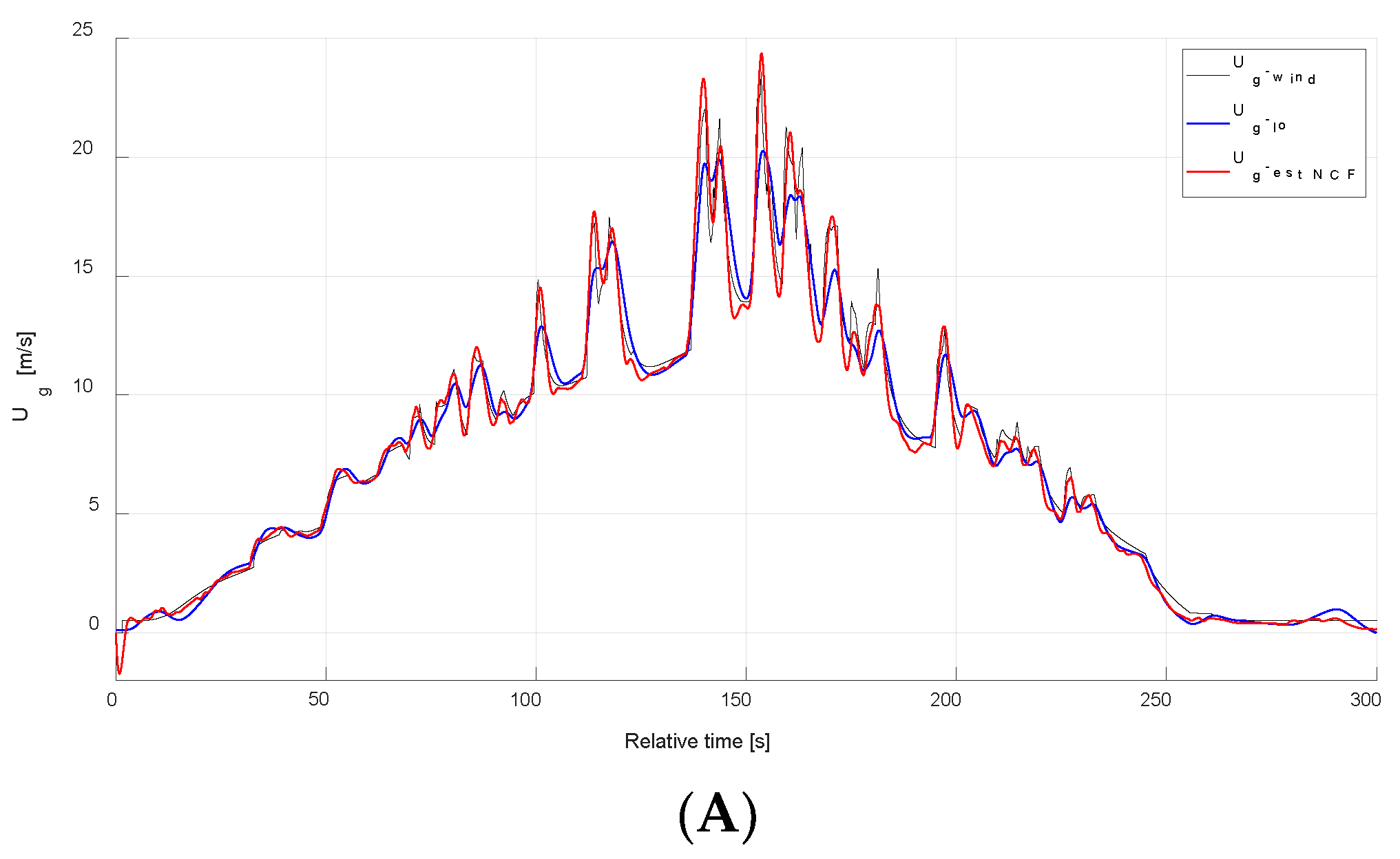
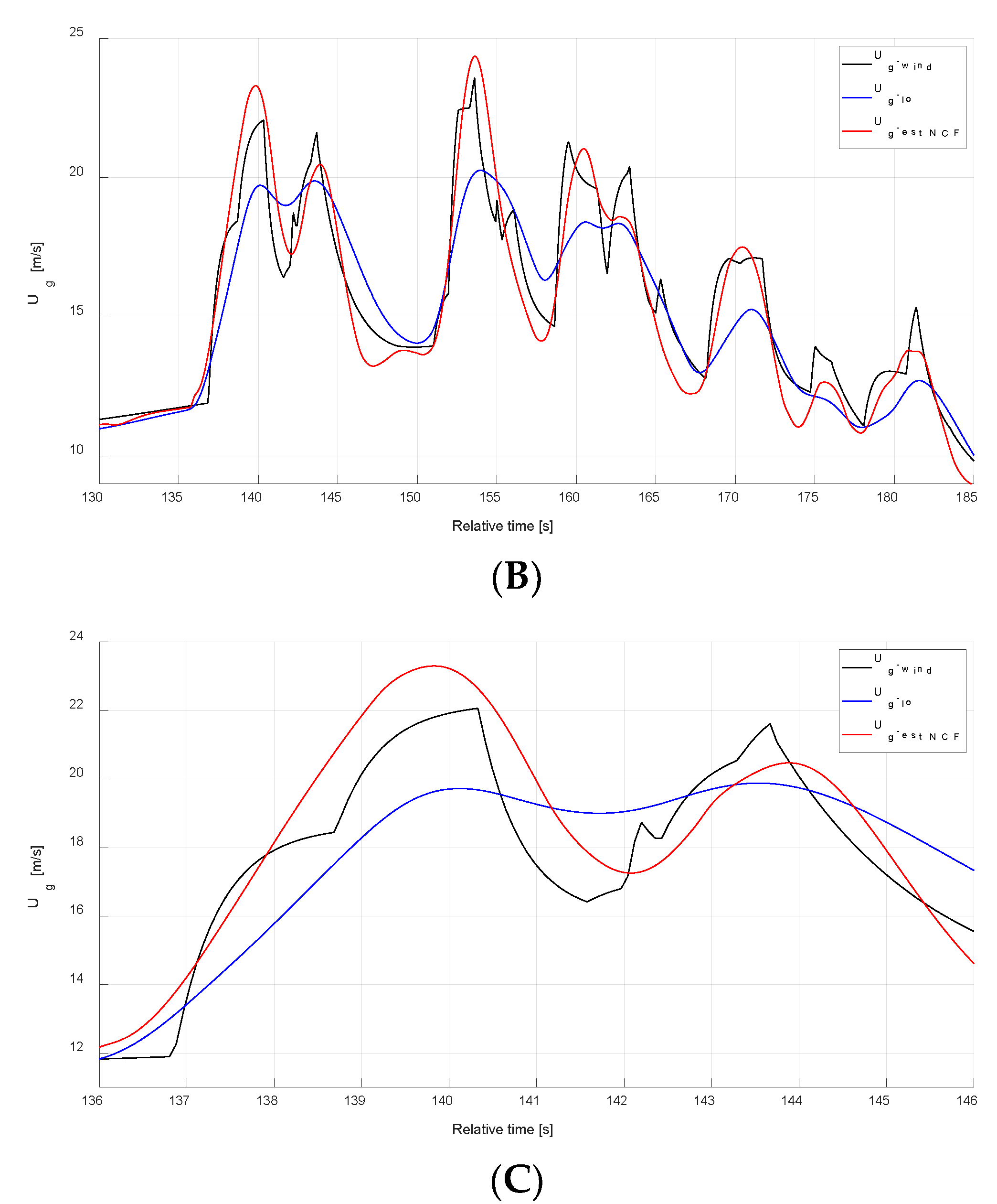
2.3. The Use of a Non-Linear Complementary Filter for Estimation of Headwind Gusts

The general structure of an NCF (Figure 4) consists of low- and high-frequency inputs of the composite signal.
The non-linear CF (NCF) is based on the proportional–integral controller, in which the proportional part manages the low-frequency input and the integral part handles the high-frequency signal. K p and K i indicate the proportional and integral gain, respectively [27]. The non-linear complementary filter transfer function is represented by Equation (14). The amplitude and phase shift of the NCF is presented in Figure 5.
E S T = K p · s + K i s 2 + K p · s + K i · L F + s 2 s 2 + K p · s + K i · H F
Taking into consideration dependencies (1), (2), (12), (13) and (17), the complete law of headwind estimation (including temporary gusts) can be formulated as (18), and finally, as Equation (19).
U g - e s t _ N C F = K p · s + K i s 2 + K p · s + K i · U g - l o + s 2 s 2 + K p · s + K i · u g - h i
U g - e s t _ N C F = K p · s + K i s 2 + K p · s + K i · ( G S x T A S ) + s 2 s 2 + K p · s + K i · ( k 1 · q ˙ k 2 · q + k 3 · δ H + k 4 · u )

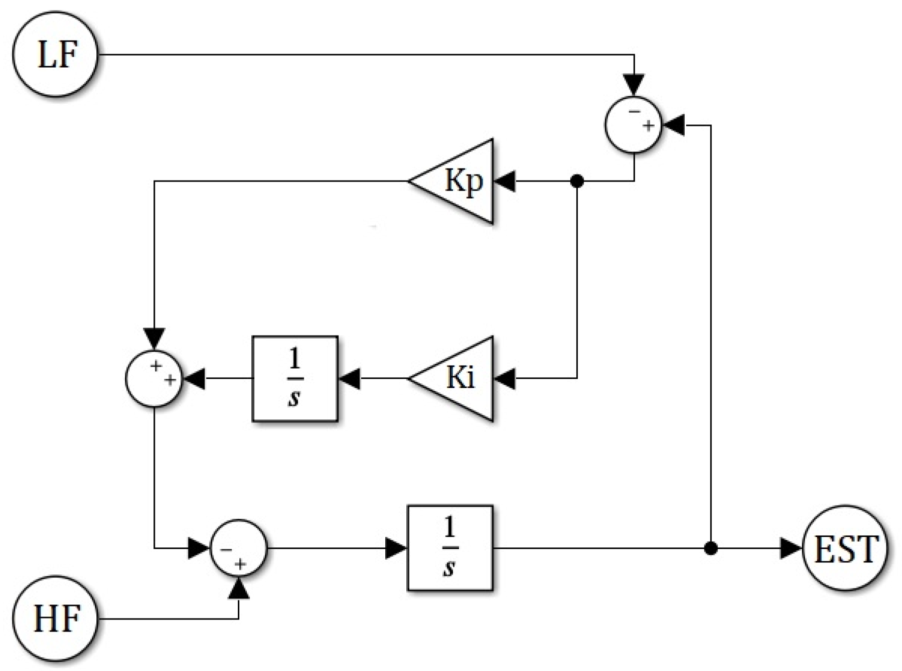
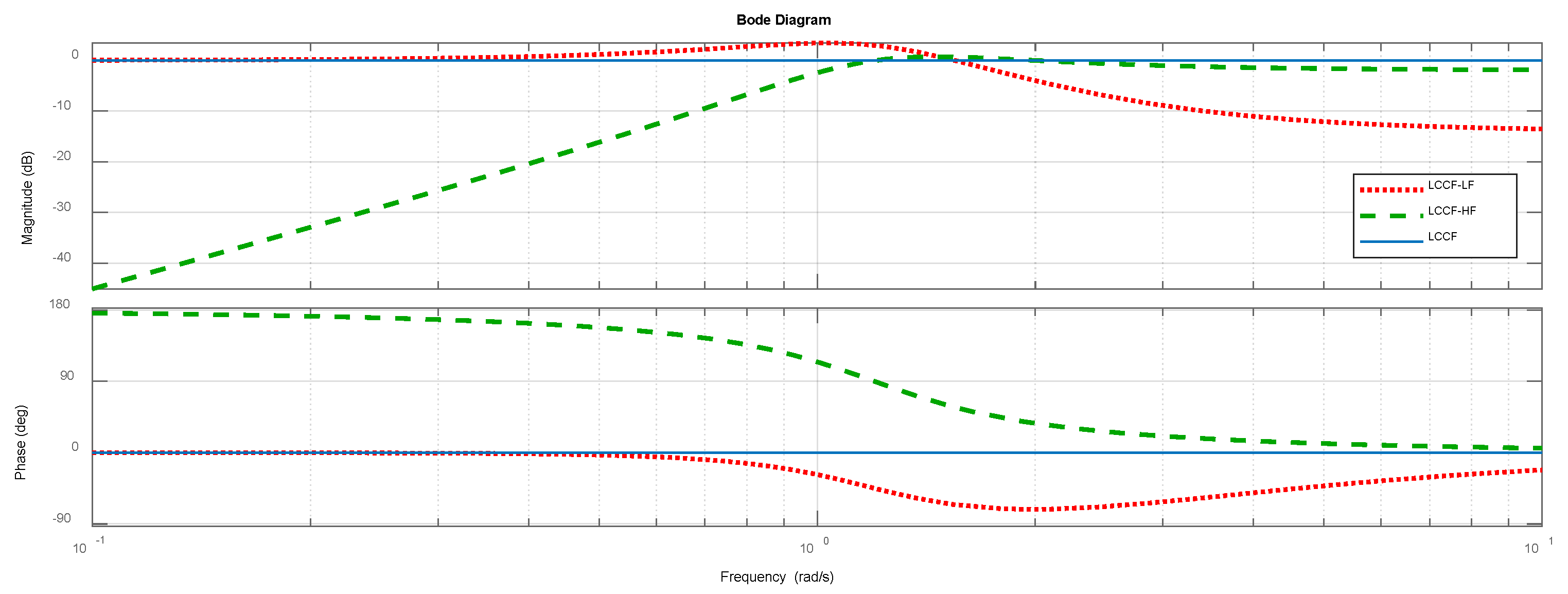
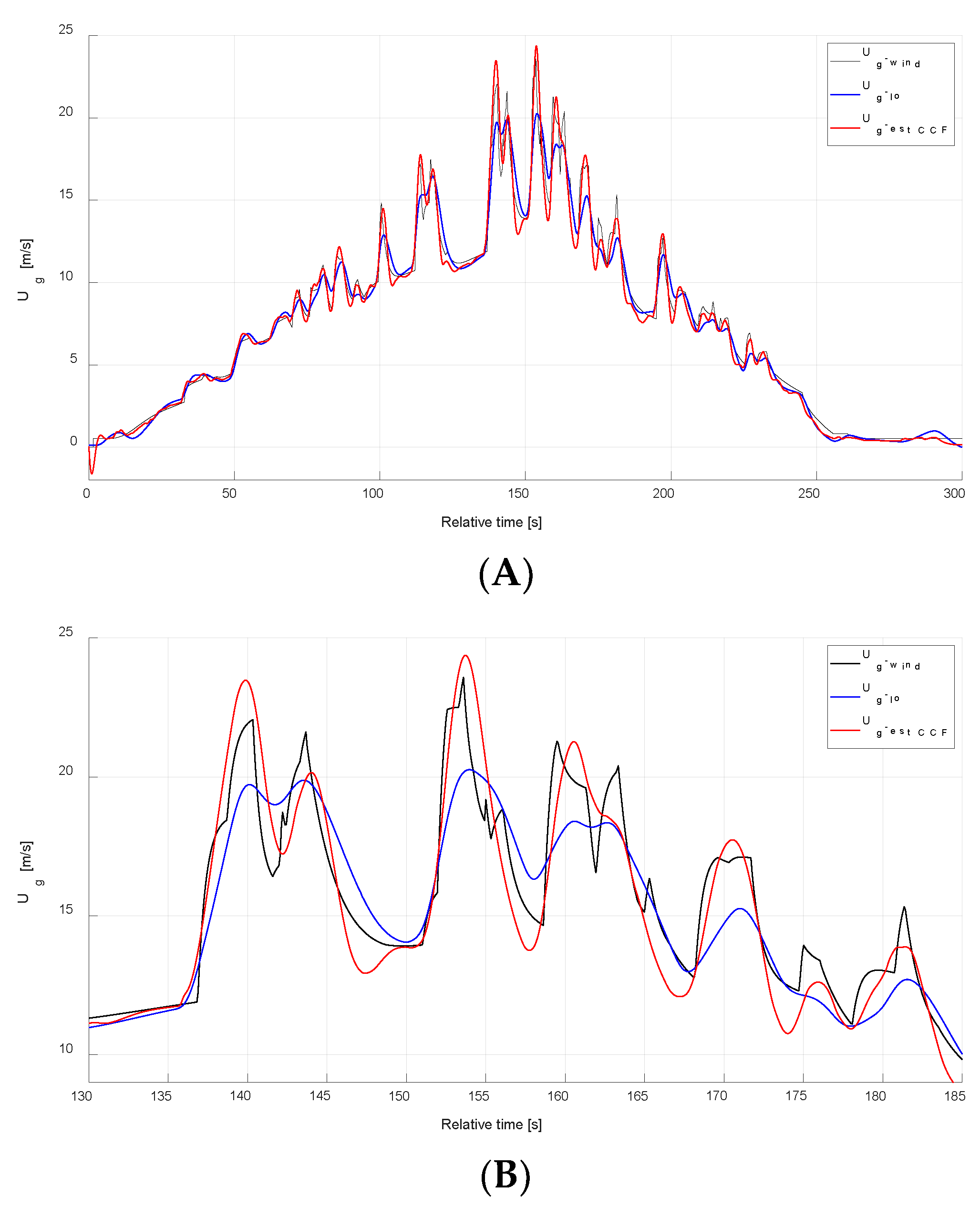
2.4. The Use of a Cascaded Complementary Filter for Estimation of Headwind Gusts

A novel cascaded architecture of the complementary filter (Figure 6) employs a non-linear and linear version of the complementary filter within one framework. K p , K i , and α are the filter constants. The proposed architecture does not require any mathematical modelling of the system and is computationally inexpensive [27]. The cascaded complementary filter transfer function is represented by Equation (14). The amplitude and phase shift of the CCF is presented in Figure 7.
E S T = ( 1 α ) · s 2 + α · K p · s + α · K i s 2 + α · K p · s + α · K i · L F + α · s 2 s 2 + α · K p · s + α · K i · H F
Referring to the dependencies (1), (2), (12), (13) and (20), the complete law of headwind estimation (including temporary gusts) can be formulated as (21), and finally, as Equation (22).
U g - e s t _ C C F = ( 1 α ) · s 2 + α · K p · s + α · K i s 2 + α · K p · s + α · K i · U g l o + α · s 2 s 2 + α · K p · s + α · K i · u g h i
U g - e s t _ C C F = ( 1 α ) · s 2 + α · K p · s + α · K i s 2 + α · K p · s + α · K i · ( G S x T A S ) + α · s 2 s 2 + α · K p · s + α · K i · ( k 1 · q ˙ k 2 · q + k 3 · δ H + k 4 · u )

3. Research Environment and Plan of Experiment

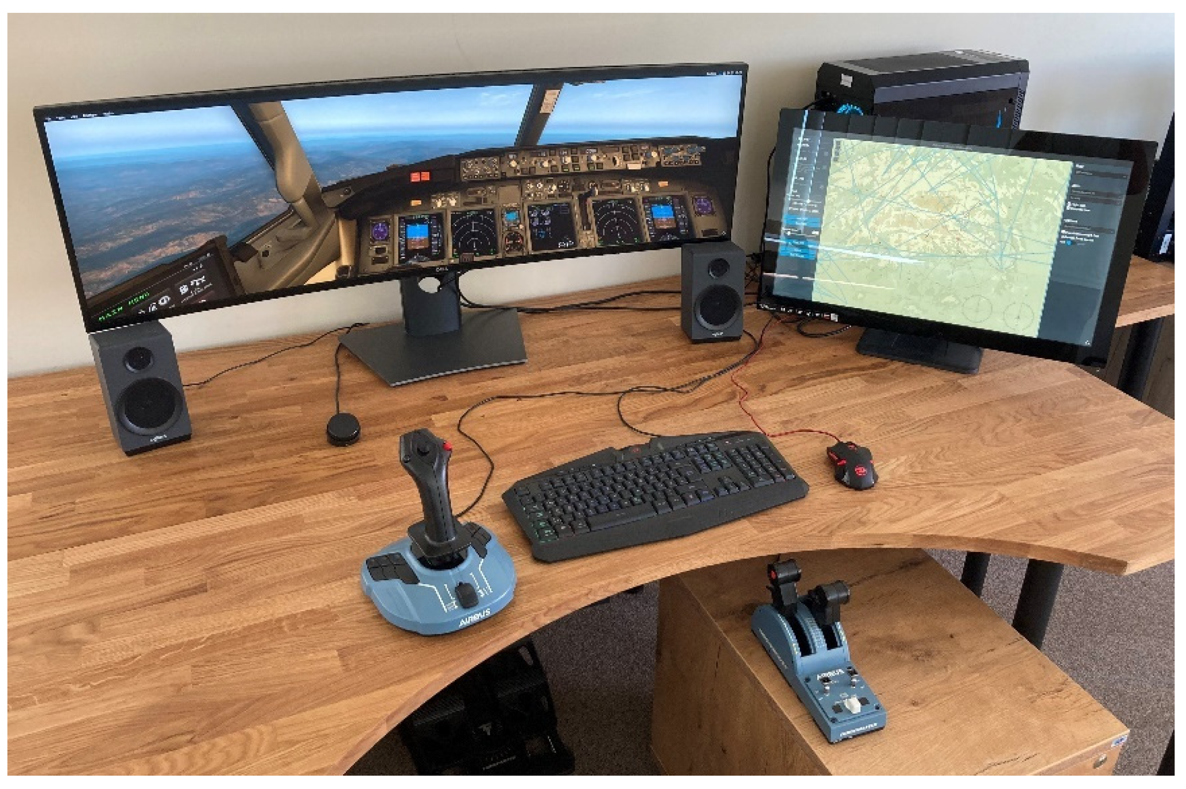
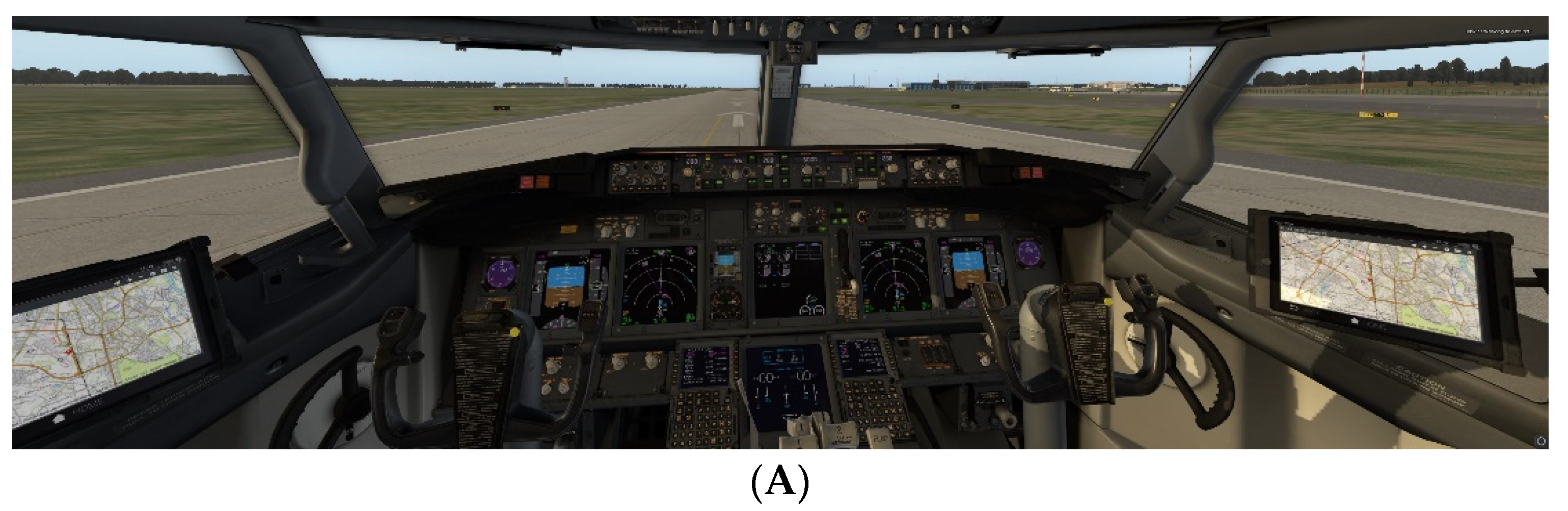
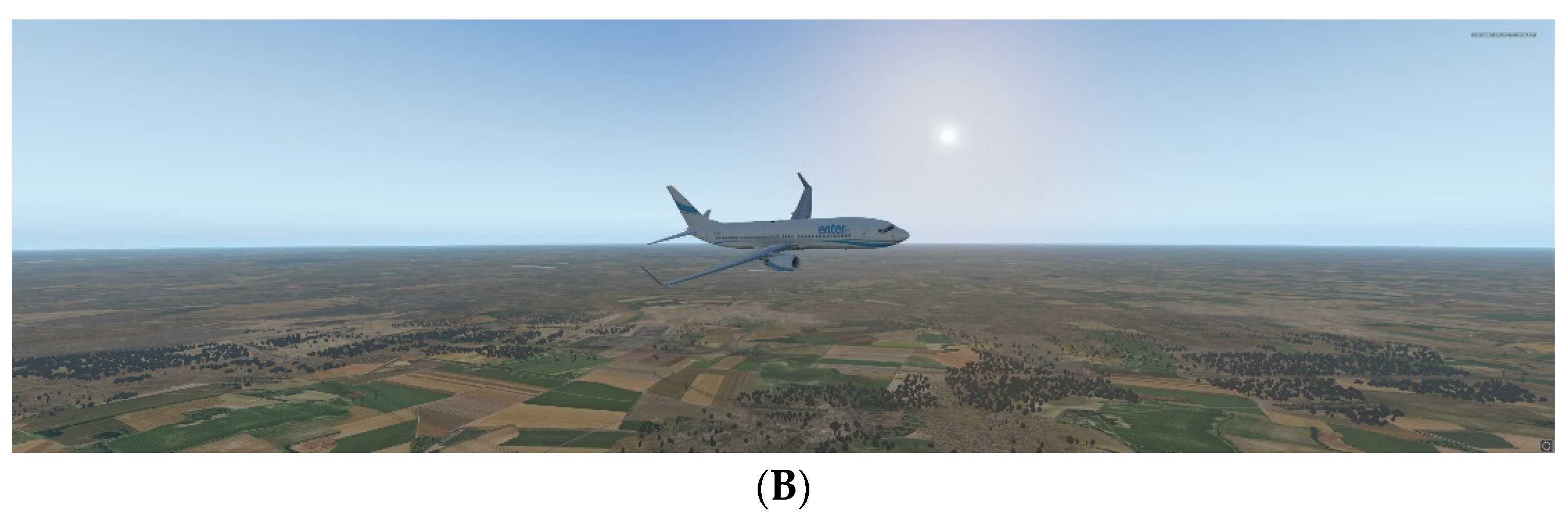
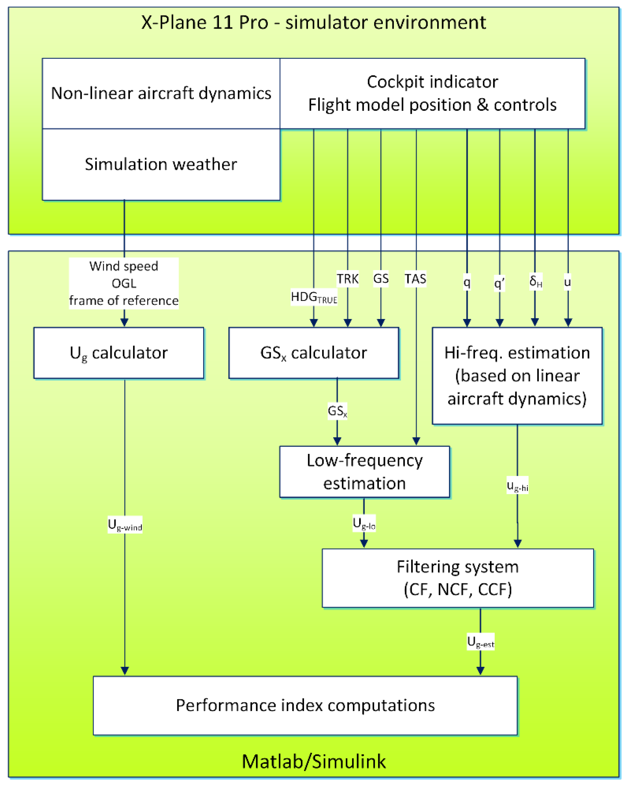
3.1. Flight Simulation Environment and Data Acquisition

A simulator stand (Figure 8) was used to assess the possibility of estimating the value of gusts with the use of the method presented in Section 2.
The block diagram of the stand is presented in Figure 9.
The flight simulation was made using the X-Plane 11 software version certified for professional use. For research purposes, layers of programmatically generated atmospheric gusts were introduced in the simulation environment. The flight parameters of one of the most popular medium-range narrow-body aircraft (B737-800) were recorded. The simulation was performed using a realistic model of this type of aircraft (Figure 10), which very accurately reflects its dynamic properties and operational functions. The analysed estimation algorithms assume the use of data available from the following on-board systems: ADIRU, GPS and flight controls systems.
A detailed summary of the recorded flight parameters, taking into account potentially available physical data sources, is presented in Table 1.
Due to the need to record flight parameters which are not available through the built-in user interface and require reference to the internal variables of the X-Plane (Datarefs), the X-Plane Communication Toolbox (XPC) was used [28]. This toolbox was launched and configured in the Matlab/Simulink environment to read internal X-Plane 11 data via UDP protocol (Figure 9). The simulations were carried out with the following assumptions:
  • Aircraft weight: 65,000 [kg];
  • Constant thrust—descent at idle thrust;
  • Automatic flight while crossing gust area;
  • Autopilot set at constant IAS = 270 kt;
  • Constant headwind direction—without crosswind and vertical gusts;
  • Simulation performed by pilot with current Type Rating on B737.
A complete diagram of the data flow in the simulation as well as in the wind parameter estimation process is shown in Figure 11.
According to this scheme, X-Plane 11 Pro simulator feeds the Matlab/Simulink environment with two types of data:
  • Information from simulated on-board systems (cockpit indicators, flight model position, and flight controls);
  • Data on the current parameters of the wind generated by the simulator environment (simulation weather).
The X-Plane 11 Pro software uses a complex non-linear model of the aircraft dynamics. Calculations for this model are performed by using the blade element theory (the airplane is divided into many small elements, and the forces acting on each element are calculated with a frequency of several or several dozen hertz) [29,30]. This model takes into account complex environmental conditions, including the effects of wind and gusts. Wind parameters can be defined using, e.g., the instructor’s station module (visible on the right in Figure 8). For individual layers of the atmosphere, we can define the wind direction, its speed, and gusts. The wind parameters obtained at the output of the model are given in the coordinate system characteristic for the Open GL graphic environment (Figure 11). For this reason, in this study, they had to be converted into the coordinate system associated with the airplane (in particular, the Ug-wind component was determined—see Figure 1).
The data required for the estimation are provided to Matlab/Simulink from the X-Plane simulator blocks responsible for on-board measurements and indications of flight parameters (Figure 11), such as: HDGTRUE, TRK, GS, TAS, q, q ˙ , δH, and u. The first three parameters are used to calculate the GSx, which together with the TAS, enable the low-frequency estimation of Ug-lo (1). The next parameters (q, q ˙ , δH, and u) feed the high-frequency estimation system. This system calculates Ug-hi using the linear mathematical equation describing the longitudinal motion of the airplane (12). Block CF/NCF/CCF generates output Ug-est using Ug-lo and Ug-hi as input signals. Finally, the performance index (detailed in Section 4.3) is calculated from the reference (ideal) value of Ug-wind and the estimated value of Ug-est.

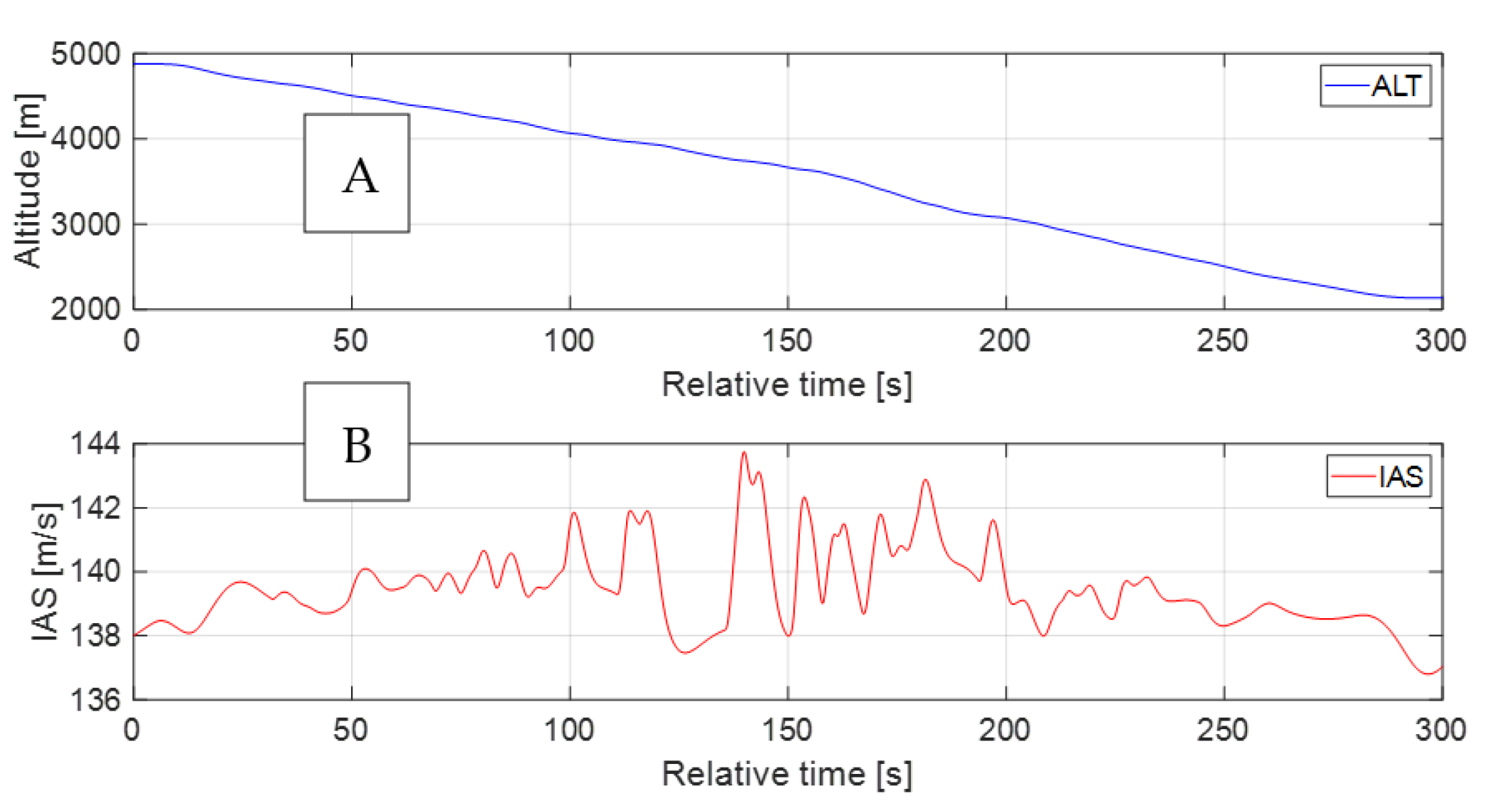
3.2. Flight Plan and Its Realisation

During the flight, the airplane descended from an altitude (ALT) of 4900 m to 2100 m (Figure 12).
The flight was fully automatic with the use of the autopilot mode—Level Change (LVL CHG). The LVL CHG mode coordinates pitch and thrust commands to make automatic climbs and descents to preselected altitudes at selected airspeeds. In case of descent, the auto-throttle mode annunciates RETARD (reversed thrust) followed by ARM. Then, auto-throttle holds idle thrust and the Autopilot Flight Director System (AFDS) holds a selected airspeed [12]. In this case, the constant IAS 270 kt (138.9 m/s) was set using the mode control panel (MCP).
The fluctuations in the indicated airspeed (IAS) in relation to the autopilot setting value of 270 kt resulted at the beginning and at the end of the simulation from transient states (start of descent and alignment to level flight, respectively). The largest fluctuations in the middle part of the recording (Figure 12B) were caused by strong atmospheric gusts.
There were no wind effects above 4900 m and below 2400 m since the airplane descended below 4900 m, but the headwind speed increased—Ug (Figure 13A,B). With wind speeds exceeding 5.1 m/s, sudden gusts of up to 23.2 m/s began. This happened between the 50th and 225th second of the simulation. Headwind and gusts decreased (225–250 s) until they reached windless conditions below an altitude of 2400 m.
The recorded data served as input data for the gust estimation system developed in the Matlab/Simulink package (MathWorks, Inc., Middlesex County, MA, USA) (Figure 14). The scheme takes into account the dependencies (1) and (12), as well as the filtration system. The CF, NCF, or CCF were used alternately in the estimation process. For comparison purposes, a delay block was implemented for the actual headwind values. The process of measuring state variables, as well as the associated estimation process (complementary fusion), in practice, is characterised by a certain delay. As it was established later in the work, the delay for the selected values of the estimation system parameters ranged from 1–1.5 s.

4. Results

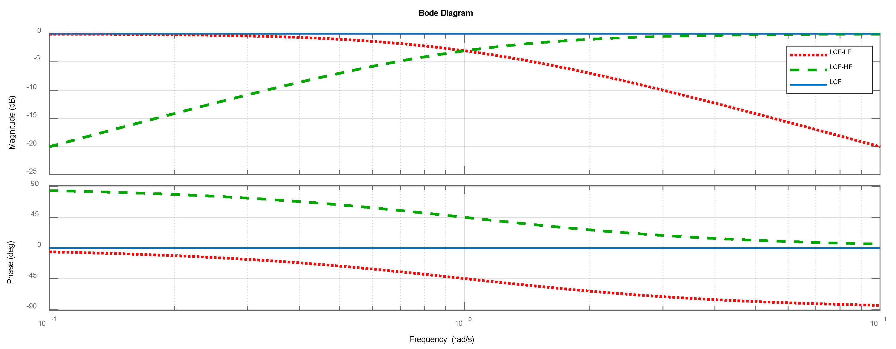
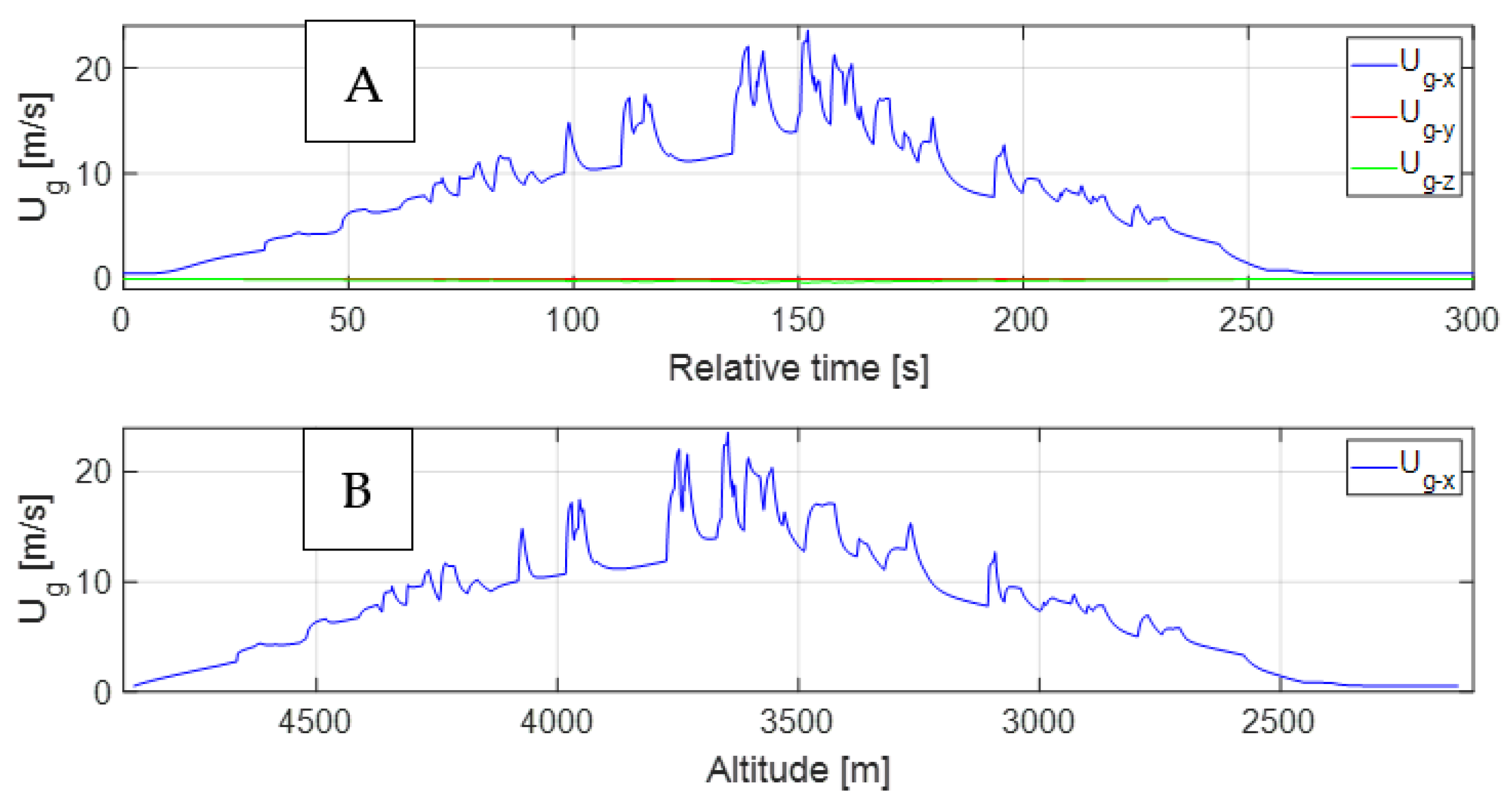
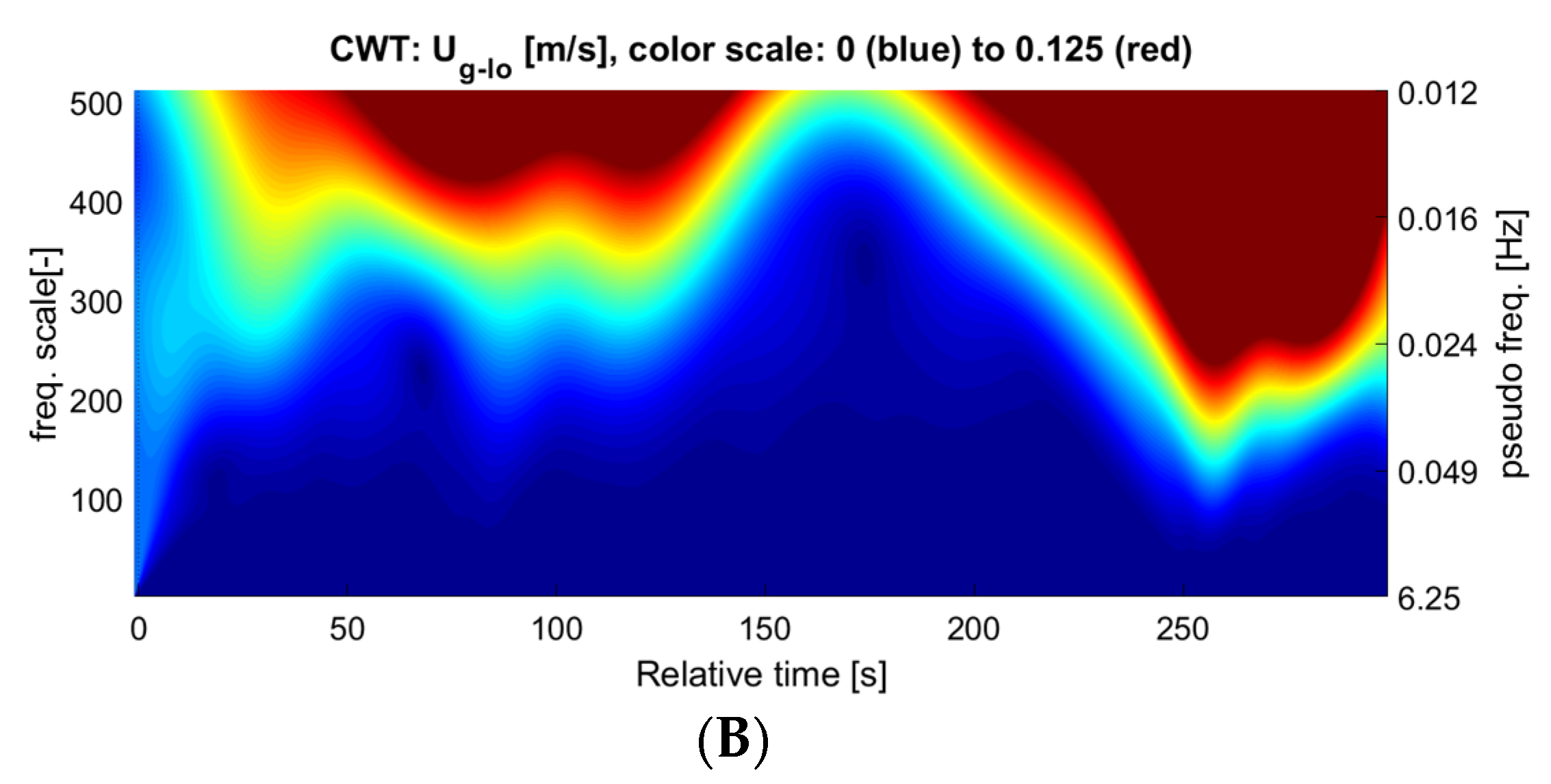
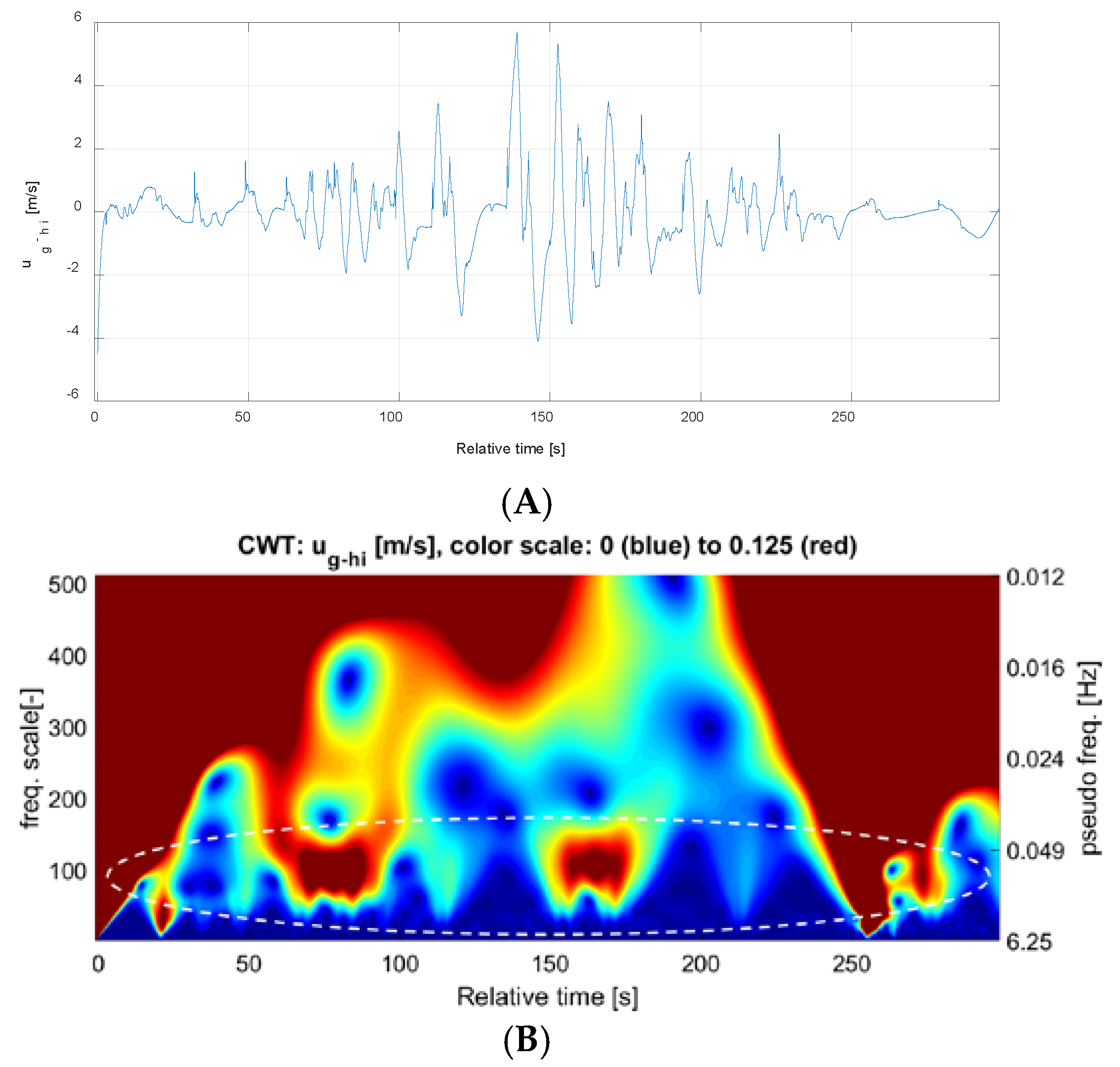
4.1. Frequency Analysis of Signals Selected for Estimation

In order to verify the nature of the variability of signals obtained on the basis of Equations (1) and (12), an analysis of the signals obtained from the flight simulator was performed. The estimation results are presented in the form of time charts (Figure 15A and Figure 16A). The conducted wavelet analysis [31] confirmed the assumptions that the estimation based on Equation (1) would be represented by a slow-varying (LF) signal (Figure 15B), while applying the dependencies of Equation (12) would make it possible to obtain an estimate containing components with much higher frequencies (Figure 16B).
The results of this preliminary analysis indicate the correctness of the theoretical considerations. Section 4.2 presents the practical result of the fusion of these two signals.

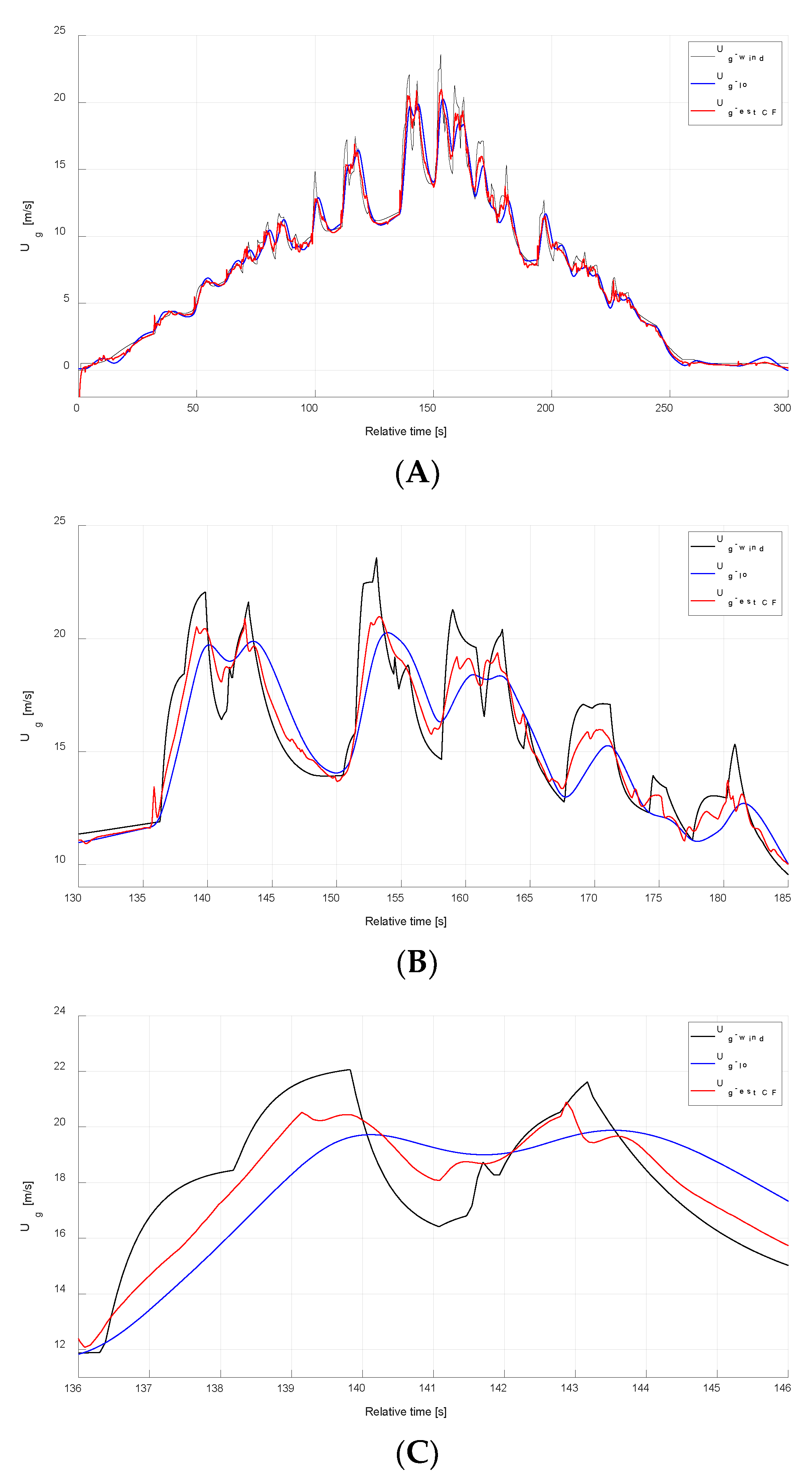
4.2. Comparison of the Estimation to Recorded Gusts

The graphs presented in this section allow us to graphically illustrate the ideal case of measurement in comparison to the obtained low-frequency signal Ug-lo and full estimation Ug-hi (fusion of low- and hi-frequency signals through selected filtration systems executed). Three ranges of the considered data were selected for the graphic presentation and computational analyses: whole simulation (time of simulation 0–300 s), several selected gusts (time of simulation 130–185 s), and single selected gust (time of simulation 136–146 s). The results presented for CF take into account the influence of changes in the time constant Ts on the result of the estimation. The graphs presented in Figure 17, Figure 18 and Figure 19 show the results of successive estimates for the three selected values of the time constant Ts = {0.5 s, 1 s, 1.5 s}. An increase in the time constant from 0.5 s to 1 s allowed for a significant improvement in adjusting the estimation to the ideal measurement of headwind gusts (Figure 17 vs. Figure 18).
On the other hand, an increase in the time constant to 1.5 s resulted in an overestimation of the maximum gust values (Figure 18 vs. Figure 19). The best qualitative and quantitative results (a detailed analysis of the obtained estimation results based on the selected performance index was carried out in Section 4.3) were obtained for Ts = 1 s (Figure 18). It should be emphasised here that the estimated signals (Ug-lo oraz Ug-est) were in fact delayed by 1 s in relation to the reference measurements. This delay was reduced in the off-line data analysis process in order to be able to accurately compare the nature of the obtained signals. In the real-time estimation system, this delay would of course occur, and it is mandatory to take into account its impact in, e.g., the aircraft control process.
Figure 20 and Figure 21 show the graphs of the estimation of the speed of the headwind gusts using the NCF and CCF filters, respectively. The charts show the most favourable results for the parameters K p = 1.2 , K i = 1.8 (NCF) and K p = 1.2 , K i = 1.8 , α = 0.8 (CCF). In the case of the NCF and CCF, output signals (Ug-lo and Ug-est) were delayed by 1.5 s compared to the ideal signals (for CF, this delay was 1 s). The NCF and CCF also made it possible to estimate headwinds relatively well; however, precisely reproducing the short-term phenomena turned out to be a bit more problematic.

4.3. Discussion

Visual assessment of the charts allows for a general (qualitative) description of the accuracy of the estimation of the headwind gust value. In order to accurately (quantitatively) compare the estimation results with the reference signal, a performance index was defined. It enables analytical comparison of the estimation results considered in Section 4.2, obtained with the use of various filtration systems. The performance index assumes the calculation of the absolute value of the difference between the values of the ideal gust measurement (recorded directly in the flight simulator environment) and the results of numerical estimation. The averaged value of matching the results to the ideal measurement was obtained by dividing the sum of these differences by the amount of data in the considered measurement range. The formulas for quantifying the math of the low-frequency estimation and complete estimation signal to the reference signal are presented in Equations (23) and (24), respectively.
Definition of performance index for low-frequency estimation of headwind gust:
W g - l o = | U g - w i n d U g - l o | N u m b e r   o f   d a t a
Definition of performance index for complete estimation of headwind gust:
W g - e s t = | U g - w i n d U g - e s t | N u m b e r   o f   d a t a
The data ranges identical to those presented in the Figure 17, Figure 18, Figure 19, Figure 20 and Figure 21 were considered in the analyses presented in this section. Detailed results are presented in the tables (Table 2, Table 3 and Table 4).
The tables show the calculation results of the headwind gust performance indices for five time constants of the complementary filter (starting from Tc = 0.1 s to Tc = 2 s), non-linear complementary filter, and cascaded complementary filter. The following tables take into account different delay values between the reference signal and the estimated signals. Table 2 presents the obtained values of the performance index for a delay of 1 s. With the time constant Tc = 1 s, the best (smallest) performance index values for the CF were obtained (these values are distinguished by bold). It should be added that the analyses were also carried out for lower and higher values of delays, but no better results were obtained. For the NCF and CCF, the best fit values in the entire range of the analysed simulation were obtained taking into account the delay of 1.5 s (Table 3). In the case of limiting the scope of analyses to only one characteristic headwind gust, a slightly better fit was obtained when taking into account the delay of 1.75 s (Table 4).

5. Conclusions

The problem of estimating atmospheric gusts is very important from the perspective of issues related to aircraft control and also flight safety in general. For example, more accurate information about the headwind gusts may improve the performance of the auto-throttle and wind shear warning systems. The conducted flight simulations made it possible to compare the estimates with the ideal case of wind measurement. Execution tests like those presented in the paper in a real environment are difficult and involves the use of specialized measuring equipment. Installation of additional equipment on an airplane results in many practical problems, e.g., certification and obtaining formal approvals, as well as high costs. Another class of problems is it being unpredictable, unique, and difficult to measure atmospheric disturbances caused by natural factors as well as wake turbulence of other aircraft. On the other hand, in the simulation environment, we were able to check the developed methods only with the accuracy of the simulation model used. In the future, if possible, it is planned to conduct tests on a certified Class D FFS simulator.
Initially, the study also considered the possibility of applying the signals from accelerometers to the estimation of wind gusts. However, after conducting preliminary research, it turned out that the method proposed in this paper allowed us to obtain more accurate results. The estimation method described in this article is characterised by a relatively precise representation of the original signal, as shown in Section 4. However, the signal delay may be troublesome, which in the estimation process carried out in real time, may reach the value of 1–1.5 s according to our analyses. The delay value was influenced in this case by the use of signals from simulated on-board instruments. Reading the parameters directly from the simulator core, bypassing on-board systems, would give ideal but not real results, while the data from on-board sensors are characterised by static and dynamic measurement errors [32]. For the analyses of airplane class, the 1–1.5 s delay in the real-time estimation of the headwind gust seemed to be an acceptable value. Nevertheless, in future research, the authors intend to use fusion methods and compensation algorithms that minimise these delays. At the end of the conclusions, one more limitation of the presented method should be mentioned. The proposed estimation algorithm is very sensitive to flight conditions and airplane configuration. For a transport aircraft, however, it seems to be possible to build an adaptive estimation system. Future work should assume the implementation of such a solution.

Author Contributions

Conceptualization, P.S. and P.R.; methodology, P.S. and P.R.; software, P.S. and P.R.; validation, P.S., T.R. and P.R.; formal analysis, P.S., T.R. and P.R.; investigation, P.S. and P.R.; resources, P.S., T.R. and P.R.; data curation, P.S. and P.R.; writing—original draft preparation, P.S. and P.R.; writing—review and editing, P.S. and P.R.; visualization, P.S. and P.R.; supervision, P.R.; project administration, P.S., T.R. and P.R.; funding acquisition, T.R. and P.R. All authors have read and agreed to the published version of the manuscript.

Funding

This research received no external funding.

Institutional Review Board Statement

Not applicable.

Informed Consent Statement

Not applicable.

Data Availability Statement

The data presented in this study are available on request from the corresponding author.

Conflicts of Interest

The authors declare no conflict of interest.

References

  1. ICAO. Manual on Low-Level Wind Shear; Doc 9817 AN/449; International Civil Aviation Organization: Montréal, QC, Canada, 2005; IBSN 92-9194-609-5. [Google Scholar]
  2. Brandl, A.; Battipede, M. Maneuver-Based Cross-Validation Approach for Angle-of-Attack Estimation. In Proceedings of the 14th WCCM-ECCOMAS Congress, Online, 11–15 January 2020; Volume 1700. [Google Scholar]
  3. Krusiec, G. On-Board Wind Shear Warning System. Master’s Thesis, Rzeszów University of Technology, Rzeszów, Poland, 2010. [Google Scholar]
  4. O’Connor, A. Demonstration of a Novel 3-D Wind Sensor for Improved WindShear Detection for Aviation Operations. Master’s Thesis, Technological University Dublin, Dublin, Ireland, 2018. [Google Scholar] [CrossRef]
  5. O’ Connor, A. Using a Wind Urchin for Airport Wind Measurements, Irish Meteorological Society. Available online: https://irishmetsociety.org/ (accessed on 19 June 2022).
  6. FAA. Windshear Weather. W: FAA, Wind Shear Training Aid; Federal Aviation Authority: Washington, DC, USA, 1990; Volume 2, p. 1133.
  7. Kelley, N.D.; Jonkman, B.J.; Scott, G.N. Comparing Pulsed Doppler LIDAR with SODAR and Direct Measurements for Wind Assessment; National Renewable Energy Laboratory: Los Angeles, CA, USA, 2007. [Google Scholar]
  8. The Boeing Company. 787 Flight Crew Operations Manual; The Boeing Company: Seattle, WA, USA, 2020. [Google Scholar]
  9. Fezans, N.; Joos, H.-D.; Deiler, C. Gust load alleviation for a long-range aircraft with and without anticipation. CEAS Aeronaut. J. 2019, 10, 1033–1057. [Google Scholar] [CrossRef] [Green Version]
  10. Prudden, S.; Fisher, A.; Marino, M.; Mohamed, A.; Watkins, S.; Wild, G. Measuring wind with small unmanned aircraft systems. J. Wind. Eng. Ind. Aerodyn. 2018, 176, 197–210. [Google Scholar] [CrossRef]
  11. IATA. Go-Around Safety Forum–Findings and Conclusions, Brussels, International Air Transport Association; IATA: Montreal, QC, Canada, 2013. [Google Scholar]
  12. Yeh, Y.C. Safety critical avionics for the 777 primary flight controls system. In Proceedings of the 20th Digital Avionics Systems Conference (Cat. No. 01CH37219), Daytona Beach, FL, USA, 14–18 October 2001; Volume 1, p. 1C2-1. [Google Scholar]
  13. Brady, C. The Boeing 737 Technical Guide; Lightning Source: La Vergne, TN, USA, 2018. [Google Scholar]
  14. Tomczyk, A. Zastosowanie Analitycznej Redundancji Pomiarów w Układzie Sterowania i Nawigacji Statku Powietrznego (Application of Analytical Redundancy of Measurements in Aircraft Control and Navigation System). In Proceedings of the Scientific Aspects Concerning Operation of Manned and Unmanned Aerial Vehicles, Dęblin, Poland, May 2015. [Google Scholar]
  15. Hall, A.P.; Marton, T.F.; Muren, P. Passive Local Wind Estimator. U.S. Patent US20140129057A1, 8 May 2014. [Google Scholar]
  16. Hall, A.P.; Marton, T.F.; Muren, P. Passive Local Wind Estimator. U.S. Patent US9031719B2, 12 May 2015. [Google Scholar]
  17. Kumon, M.; Mizumoto, I.; Iwai, Z.; Nagata, M. Wind estimation by unmanned air vehicle with delta wing. In Proceedings of the 2005 IEEE International Conference on Robotics and Automation IEEE, Barcelona, Spain, 18–22 April 2005; pp. 1896–1901. [Google Scholar]
  18. Meier, K.; Hann, R.; Skaloud, J.; Garreau, A. Wind Estimation with Multirotor UAVs. Atmosphere 2022, 13, 551. [Google Scholar] [CrossRef]
  19. Reuder, J.; Jonassen, M.O.; Ólafsson, H. The Small Unmanned Meteorological Observer SUMO: Recent developments and applications of a micro-UAS for atmospheric boundary layer research. Acta Geophys. 2012, 60, 1454–1473. [Google Scholar] [CrossRef]
  20. Brezoescu, A.; Castillo, P.; Lozano, R. Wind estimation for accurate airplane path following applications. J. Intell. Robot. Syst. 2014, 73, 823–831. [Google Scholar] [CrossRef]
  21. Wingrove, R.C.; Bach, R.E., Jr. Severe turbulence and maneuvering from airline flight records. J. Aircr. 1994, 31, 753–760. [Google Scholar] [CrossRef]
  22. Dołęga, B.; Kopecki, G.; Tomczyk, A. Analytical redundancy in control systems for unmanned aircraft and optionally piloted vehicles. Pr. Inst. Lotnictwa 2017, 2017, 31–44. [Google Scholar] [CrossRef] [Green Version]
  23. Kopecki, G.; Tomczyk, A.; Rzucidło, P. Algorithms of measurement system for a micro UAV. Solid State Phenom. 2013, 198, 165–170. [Google Scholar] [CrossRef]
  24. Dąbrowski, W.; Popowski, S. Estimation of wind parameters on flying objects. Pomiary Autom. Robot. 2013, 17, 552–557. [Google Scholar]
  25. Rautenberg, A.; Graf, M.S.; Wildmann, N.; Platis, A.; Bange, J. Reviewing Wind Measurement Approaches for Fixed-Wing Unmanned Aircraft. Atmosphere 2018, 9, 422. [Google Scholar] [CrossRef] [Green Version]
  26. Bociek, S.; Gruszecki, J. Automatic Aircraft Control Systems; Oficyna Wydawnicza Politechniki Rzeszowskiej: Rzeszów, Poland, 1999. (In Polish) [Google Scholar]
  27. Narkhede, P.; Poddar, S.; Walambe, R.; Ghinea, G.; Kotecha, K. Cascaded Complementary Filter Architecture for Sensor Fusion in Attitude Estimation. Sensors 2021, 21, 1937. [Google Scholar] [CrossRef]
  28. X-Plane Communication Toolbox (XPC). Available online: https://software.nasa.gov/software/ARC-17185-1 (accessed on 27 April 2022).
  29. Yu, L.; He, G.; Zhao, S.; Wang, X.; Shen, L. Design and Implementation of a Hardware-in-the-Loop Simulation System for a Tilt Trirotor UAV. J. Adv. Transp. 2020, 2020, 4305742. [Google Scholar] [CrossRef]
  30. Bittar, A.; Figuereido, H.V.; Guimaraes, P.A.; Mendes, A.C. Guidance software-in-the-loop simulation using x-plane and simulink for UAVs. In Proceedings of the 2014 International Conference on Unmanned Aircraft Systems (ICUAS), Orlando, FL, USA, 27–30 May 2014; pp. 993–1002. [Google Scholar]
  31. Bakunowicz, J.; Rzucidło, P. Detection of Aircraft Touchdown Using Longitudinal Acceleration and Continuous Wavelet Transformation. Sensors 2020, 20, 7231. [Google Scholar] [CrossRef] [PubMed]
  32. Welcer, M.; Szczepański, C.; Krawczyk, M. The Impact of Sensor Errors on Flight Stability. Aerospace 2022, 9, 169. [Google Scholar] [CrossRef]
Figure 1. Illustration of relations from Equation (1).
Applsci 12 06349 g001
Figure 2. Complementary filter diagram.
Applsci 12 06349 g002
Figure 3. Bode diagram (amplitude and phase) for linear CF.
Applsci 12 06349 g003
Figure 4. Non-linear complementary filter diagram.
Applsci 12 06349 g004
Figure 5. Bode diagram (amplitude and phase) for non-linear CF.
Applsci 12 06349 g005
Figure 6. Cascaded complementary filter diagram.
Applsci 12 06349 g006
Figure 7. Bode diagram (amplitude and phase) for cascaded complementary filter.
Applsci 12 06349 g007
Figure 8. Stationary simulator station.
Applsci 12 06349 g008
Figure 9. Block diagram of the stand for flight simulation and data acquisition.
Applsci 12 06349 g009
Figure 10. (A) External view of a jet airliner—Boeing 737–800—during simulation; (B) cockpit view of a jet airliner—Boeing 737–800.
Applsci 12 06349 g010aApplsci 12 06349 g010b
Figure 11. Flight simulation and wind parameter estimation—data flow scheme.
Applsci 12 06349 g011
Figure 12. (A) Altitude and (B) IAS recorded during simulated flight.
Applsci 12 06349 g012
Figure 13. Registered ideal gust measurements from simulation weather section; (A) wind speed as a function of time, (B) wind speed as a function of altitude.
Applsci 12 06349 g013
Figure 14. Scheme of system proposed for estimation of the headwind gust.
Applsci 12 06349 g014
Figure 15. (A) Absolute value of headwind speed estimation (Ug-lo) based on GSx and TAS; (B) continuous wavelet analysis of data from (A).
Applsci 12 06349 g015aApplsci 12 06349 g015b
Figure 16. (A) Temporary change of frontal wind component estimation (Ug-hi) based on Equation (12); (B) continuous wavelet analysis of data from (A).
Applsci 12 06349 g016
Figure 17. Comparison of the gust value with the estimation results (complementary filter, Tc = 0.5 s, estimation delay reduced by 1 s)—flight crossing a gust area; (A) whole simulation, (B) several selected gusts, and (C) single selected gust.
Applsci 12 06349 g017
Figure 18. Comparison of the gust value with the estimation results (complementary filter, Tc = 1 s, estimation delay reduced by 1 s)—flight crossing a gust area; (A) whole simulation, (B) several selected gusts, and (C) single selected gust.
Applsci 12 06349 g018aApplsci 12 06349 g018b
Figure 19. Comparison of the gust value with the estimation results (complementary filter, Tc = 1.5 s, estimation delay reduced by 1 s)—flight crossing a gust area; (A) whole simulation, (B) several selected gusts, and (C) single selected gust.
Applsci 12 06349 g019aApplsci 12 06349 g019b
Figure 20. Comparison of the gust value with the estimation results (non-linear complementary filter, estimation delay reduced by 1.5 s)—flight crossing a gust area; (A) whole simulation, (B) several selected gusts, and (C) single selected gust.
Applsci 12 06349 g020aApplsci 12 06349 g020b
Figure 21. Comparison of the gust value with the estimation results (cascaded complementary filter, estimation delay reduced by 1.5 s)—flight crossing a gust area; (A) whole simulation, (B) several selected gusts, and (C) single selected gust.
Applsci 12 06349 g021aApplsci 12 06349 g021b
Table 1. Parameters recorded in the X-Plane environment for the purposes of testing the headwind gust estimation algorithm.
ParameterSourceSymbol—UnitSampling Frequency
TimeSimulation timet [s]12.5 Hz
AltitudeCockpit indicatorALT [m]12.5 Hz
Indicated air speedCockpit indicatorIAS [m/s12.5 Hz
True air speedCockpit indicatorTAS [m/s]12.5 Hz
Ground speedFlight model positionGS_x [m/s]12.5 Hz
Wind speed x (OGL)Simulation weatherWind_x [m/s]12.5 Hz
Wind speed y (OGL)Simulation weatherWind_y [m/s]12.5 Hz
Wind speed z (OGL)Simulation weatherWind_z [m/s]12.5 Hz
Pitch rateFlight model positionQ [deg/s]12.5 Hz
Pitch angular accelerationFlight model positionQ_dot [deg/s2]12.5 Hz
Horizontal Stabilizer
elevator deflection
Flight model controlsHS_elev [deg]12.5 Hz
Table 2. The results of computation of performance indices for delay = 1 s.
Simulation Scope10 ÷ 280 s130 ÷ 185 s136 ÷ 146 s
W g - l o W g - e s t W g - l o W g - e s t W g - l o W g - e s t
CF   T c   = 0.1 s0.6214980.5761791.3498371.2362061.9636711.769485
CF   T c   = 0.5 s0.6214980.4016441.3498370.7800361.9636711.061259
CF   T c   = 0.75 s0.6214980.3315821.3498370.5807061.9636710.777876
CF   T c   = 1.0 s0.6214980.3185161.3498370.5206761.9636710.693720
CF   T c   = 1.25 s0.6214980.3598231.3498370.6190291.9636710.830859
CF   T c   = 1.5 s0.6214980.4201621.3498370.7545731.9636711.010642
CF   T c   = 2.0 s0.6214980.5515401.3498371.0288001.9636711.369436
NCF0.6214980.4780831.3498371.0908881.9636711.608529
CCF0.6214980.5212931.3498371.2020501.9636711.756727
Table 3. The results of computation of performance indices for delay = 1.5 s.
Simulation Scope10 ÷ 280 s130 ÷ 185 s136 ÷ 146 s
W g - l o W g - e s t W g - l o W g - e s t W g - l o W g - e s t
CF   T c   = 0.1 s0.5109540.4912011.0485530.9959811.3915551.304261
CF   T c   = 0.5 s0.5109540.4163041.0485530.7663021.3915550.925406
CF   T c   = 1.0 s0.5109540.4240711.0485530.7027731.3915551.053646
CF   T c   = 1.5 s0.5109540.5130631.0485530.8728851.3915551.456678
CF   T c   = 2.0 s0.5109540.6129591.0485531.0597671.3915551.852097
NCF0.5109540.4043701.0485530.8195421.3915551.063059
CCF0.5109540.4354401.0485530.9153751.3915551.219745
Table 4. The results of computation of performance indices for delay = 1.75 s.
Simulation Scope10 ÷ 280 s130 ÷ 185 s136 ÷ 146 s
W g - l o W g - e s t W g - l o W g - e s t W g - l o W g - e s t
CF   T c   = 0.1 s0.4878570.4817360.9820920.9642431.2087371.189704
CF   T c   = 0.5 s0.4878570.4701100.9820920.9019491.2087371.191916
CF   T   c   = 1.0 s0.4878570.5220650.9820920.9560121.2087371.522830
CF   T c   = 1.5 s0.4878570.6143480.9820921.1115671.2087371.861305
CF   T c   = 2.0 s0.4878570.7094090.9820921.2672761.2087372.193865
NCF0.4878570.4383720.9820920.8449021.2087371.001125
CCF0.4878570.4560160.9820920.9186671.2087371.120209
Publisher’s Note: MDPI stays neutral with regard to jurisdictional claims in published maps and institutional affiliations.

