Article

Seismic Response of Loess-Mudstone Slope with High Anti-Dip Angle Fault Zone

1
Department of Geological Engineering, Chang’an University, Xi’an 710054, China
2
Key Laboratory of Western China’s Mineral Resources and Geological Engineering, Ministry of Education, Chang’an University, Xi’an 710054, China
3
State Key Laboratory of Resources and Environmental Information System, Institute of Geographic Sciences and Natural Resources Research, Chinese Academy of Sciences, Beijing 100101, China
4
School of Water and Environment, Chang’an University, Xi’an 710054, China
*
Authors to whom correspondence should be addressed.
Appl. Sci. 2022, 12(13), 6353; https://doi.org/10.3390/app12136353
Submission received: 3 June 2022 / Revised: 19 June 2022 / Accepted: 20 June 2022 / Published: 22 June 2022
(This article belongs to the Section Civil Engineering)

Abstract

:
Earthquakes are one of the main factors inducing large-scale loess bedrock and especially loess-mudstone landslides in Western China, and these types of landslides are often closely related to fault zones. To study the influence of high anti-dip angle fault zones (HADAFZs) on loess-mudstone slopes (LMSs) during earthquakes, a scaled model with an HADAFZ of 80° using a shaking table test and numerical calculation, subjected to earthquake waves, was applied to reveal the rules of seismic response and failure characteristics. The acceleration dynamic response had a top surface amplification effect on the slope surface, an accelerated increase effect on the slope-surface hanging wall, an amplification effect away from the free slope face in the loess stratum, and a combination of elevation and lithology effects in the vertical section. At the loess–weathered mudstone (L–W) and weathered mudstone–mudstone (W–M) interfaces, the amplification response of a hanging wall was the largest, fault zone was the second, and foot wall was the smallest. Furthermore, the key value of input peak ground acceleration (PGA) for the dynamic response was a = 0.3 g. The hanging wall amplification effect became apparent while a > 0.3 g, and cracks appeared on the surface of the slope. The dynamic response of the soil pressure was influenced by the hanging wall amplification effect and had a positive correlation with the thickness of the overlying layers, both in the loess stratum and at the L–W interface. However, the dynamic soil pressure maximum variation (DSPMV) on both sides of the fault zone was larger than that in the fault zone. The development of an HADAFZ in the LMS hindered the integral connection of the potential sliding surface and restricted the overall sliding failure of the slope during the earthquakes.

1. Introduction

Western China has complex geological conditions, with active tectonics and frequent seismic activities. Between 1949 and 2009, a total of 1679 earthquakes with magnitudes greater than 5.0 occurred in China, of which 1547 (92.14%) occurred in Western China [1]. Loess is distributed widely in this region, with a distribution area of 633,500 km2 and a complex and diverse genetic type; it accounts for 6.63% of the total land area in the entire country [2]. The instability of loess slopes during earthquakes is well-researched because such instability often results in serious landslide disasters, which threaten the personal and property-related safety of the residents in the surrounding areas. For example, in 1718, 59 loess landslides with ranges greater than 500 m were induced by the Gansu Tongwei earthquake (Ms = 7.5). In 1920, a loess landslide with an area of over 4000 km2 was triggered by the Haiyuan earthquake (Ms = 8.5). More than 150 loess landslides were induced by the Gansu Yongdeng earthquake (Ms = 5.8) in 1995 [3] and on 22 July 2013, an earthquake (Ms = 6.6) in Min-Zhang County, Gansu Province, resulted in more than 600 loess landslides [4,5]. The occurrence of these earthquake-induced loess landslides is related to the existence of active fault zones, which clearly affect the distribution and development of earthquake-induced landslides in western China [6].
Many studies have been carried out on the dynamic response and stability of slopes during earthquakes. The theory of sliding liquefaction has been proposed by Terzaghi et al., Sladen et al., and Lade [7,8,9], who argue that liquefaction occurs in the sliding body under the action of forced vibration. Through dynamic triaxial liquefaction tests of loess from the central United States, loess liquefaction under cyclic dynamic loadings and seismic liquefaction slip of the loess layer were rigorously analysed by Puri, Sandoval-Shannon, Ishihara, Prakash, and Guo [10,11,12,13,14]. The finite slip displacement method was proposed by Newmark [15], which provided a new idea for the quantitative evaluation of slope dynamic stability. It was subsequently confirmed that stability evaluation using this method is reliable [16,17], and it was developed and improved by Sarma, Franklin, and Constantinou et al. [18,19,20]. Bo et al. [21] proposed an efficient finite element method, based on the quasi-static method, with which to evaluate the dynamic stability of soil slopes. Davis [22] placed monitors in Nevada, USA, and found that vibration at the high point of the terrain was stronger than that on a relatively flat area. Furthermore, investigations found that the obvious topographic amplification effect caused by the 1989 San Francisco and 1994 Pacific Northridge earthquakes was the cause of several landslides [23,24]. The factors influencing slope stability during earthquakes and the slope instability mechanism were summarised by Qi et al. [25], indicating that seismic inertia force and the building up of excess-static pore pressure are two reasons for the induction of the instability of a slope. The characteristics of the distribution of earthquake-induced landslides in loess areas and the main factors affecting such landslides were analysed by Zhang et al. [26], by building a classification model based on the AHP method and indicating that the classification model is appropriate to the loess landslide zoning.
Zhang et al. [27] carried out several ring shear tests on loess soil formed by the landslide induced by the Haiyuan earthquake to study the formation mechanism of earthquake-induced loess landslides, and they indicated that the pore pressure was built-up gradually before the failure, and after that, that large pore pressure was quickly generated due to the failure of the loess soil structure. The deformation and failure characteristics of large-scale loess landslides triggered by the 1949 Khait earthquake in Tajikistan were studied by Evans et al. [28], who indicated that the Khait landslide involved the transformation of an earthquake-triggered rockslide into a very rapid flow by the entrainment of saturated loess into its movement. Wang et al. [29] discussed the types and basic features of loess landslides induced by the Tianshui (1654), Tongwei (1718), and Haiyuan (1920) earthquakes, dividing the landslides in the valley city of the loess area into three types: homogeneous loess landslide, loess interface landslide, and loess–mudstone cutting layer landslide. Through a series of undrained triaxial compression and ring shear tests, Wang et al. [30] suggested that saturated loess was susceptible to liquefaction damage, and air trapped in the loess was not the main causal factor for large-scale landslides during the 1920 Haiyuan earthquake. Through dynamic triaxial analyses and finite element numerical calculations, the probability of liquefaction and dynamic response characteristics of several loess landslides induced by the Minxian earthquake were analysed by Wu et al. [31], who indicated that continuous heavy rain before the earthquake induced an increasing moisture content and shear strength reduction in the surface loess layer of the slope. Coupled with the strong quake, tensile stress and liquefaction occurred in the surface soil layer. The dynamic response rules of loess-mudstone slopes (LMSs) with fault zones of gentle and steep dip angles using shaking table tests were studied by Huang et al. and Jia et al. [6,32], who revealed that the seismic response and failure mode of LMSs were controlled by bedding fault zones (BFZ), indicating that the fracture distribution on the slope surface is related to the dip angle of the fault zone; the smaller the dip angle, the worse the dynamic stability. To investigate the seismic response of a bedding rock slope, a time-frequency joint analysis method was proposed by Song et al. [33], which showed that the topographic and geological conditions have great impacts on the dynamic response characteristics of the slope. Novel recurrent neural networks were applied to predict the slope dynamic response by Huang et al. [34], which showed that recurrent neural networks perform well in the analysis of the seismic dynamic response of a slope and provide better predictions than the multi-layer perceptron network. To investigate the effect of both horizontal pulse-like motion and vertical components on the dynamic response of a slope, a shaking table test was performed by Zhu et al. [35] which indicated that a vertical component has limited effect on a seismic response when the horizontal component is a pulse-like ground motion, but that it can greatly enhance the seismic response of a slope under ordinary horizontal motion.
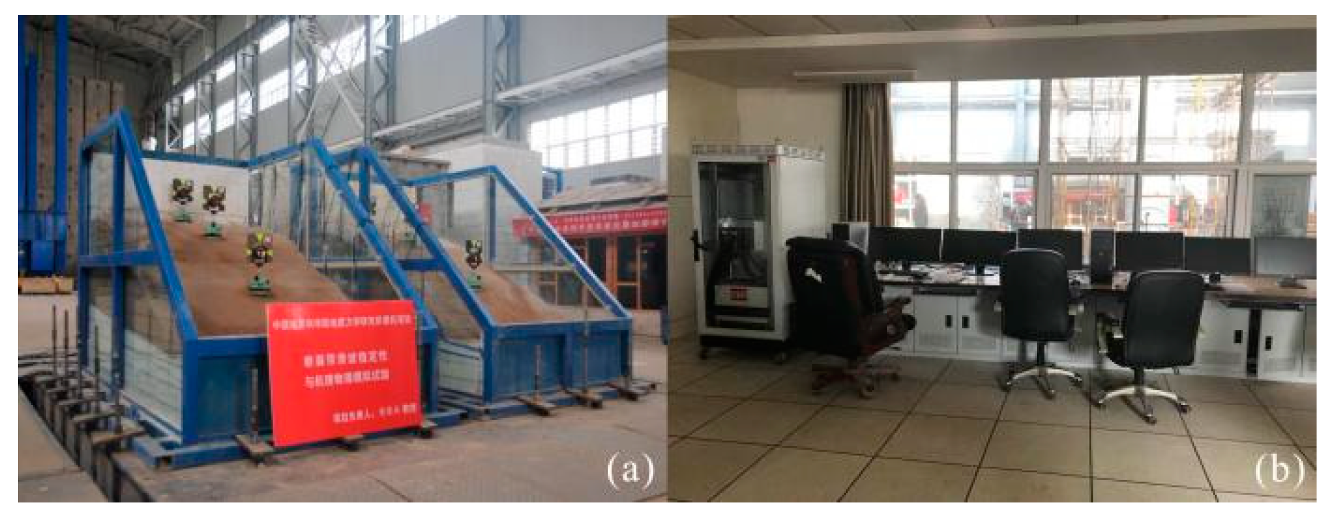
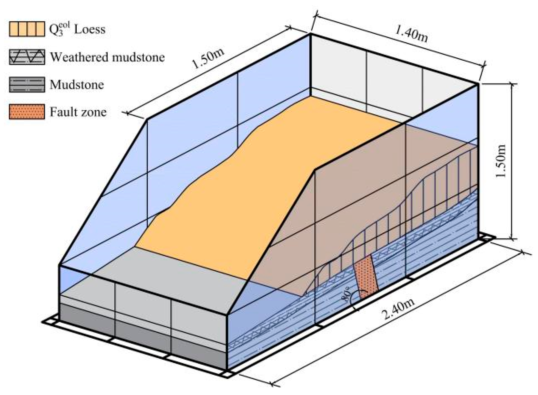
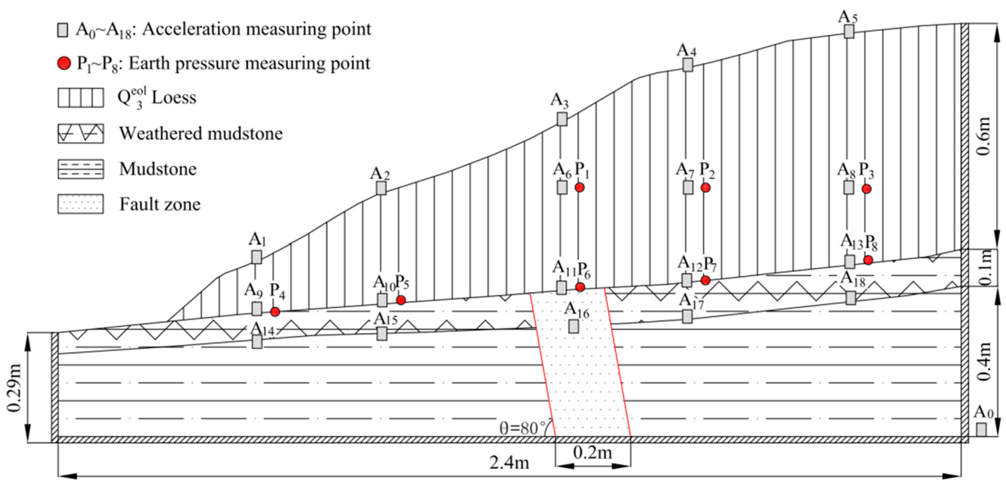
These studies mainly focused on vibration sliding liquefaction, dynamic stability evaluation, dynamic instability mechanisms, and the dynamic response characteristics of general slopes. Only a small number of studies have considered the influence of BFZ on the dynamic response of slopes. Moreover, few reports exist on the seismic response rules, deformation, and failure mechanism, along with the failure process and the mode of the LMSs with high anti-dip angle fault zones (HADAFZs) during earthquakes. Therefore, based on typical loess–mudstone landslides in the Tianshui area of Gansu Province, China, a general LMS model with an HADAFZ was constructed in this study to explore the rules of seismic response and failure for the model slope during earthquakes using a large-scale shaking table test and numerical simulation.

2. Shaking Table Test Programme

2.1. Shaking Table Equipment

The shaking table test system used in this study was produced by MTS Corporation (USA) and performed three-dimensional seismic simulations with six degrees of freedom (Figure 1). The main specifications of the shaking table are listed in Table 1. A rigid model box was used in the test which was 2.4 m in length, 1.4 m in width, and 1.5 m in height (Figure 2). To weaken the influence of the boundary effect brought by the scale model, polystyrene foam boards with 10 cm thickness were placed perpendicular to the vibration direction and lined on the front and rear sides, and a quantity of gravel was fixed with epoxy to the inside bottom of the model box. The test principle involved the earthquake wave being loaded by the computer control system, and the vibration excitation was generated by the bottom of the shaking table, which caused the model box to vibrate.

2.2. Similarity Design of the Shaking Table Test

In the test, the similitude ratio of geometry, elastic modulus, and density between the prototype and model were taken as the basic dimensions, namely C l = C E = 20.0 and C ρ = 1.0, respectively. In accordance with similarity criteria and the basic dimensions, the similar constants of other physical and mechanical parameters are listed in Table 2.

2.3. Selection of Similarity Materials

The stratum structure of the model slope from the ground surface included loess, weathered mudstone, and mudstone as well as an HADAFZ (80°) (Figure 2). The prototypical primary parameters of the loess-mudstone with the abovementioned fault zone were based on geotechnical test results of soil samples from the Houjiashan landslide in Tianshui. The primary parameter values of the model material were estimated based on the requirements of similar designs. Mixtures of prototype loess, sand, barite powder, quartz sand, gypsum, glycerine, and water were used to simulate each stratum. The quartz sand and barite powder acted as coarse and fine aggregates, respectively, the gypsum acted as a cement, and the glycerine as a water-retaining agent. To obtain a material mix ratio that met the estimated value range, multiple sets of orthogonal mix ratio tests were performed (Figure 3). The model material mix ratios that were obtained are shown in Table 3. The values of the primary parameters of the prototype and model slope strata are shown in Table 4.

2.4. Sensors in the Test

The seismic response of acceleration and soil pressure in the model slope were monitored as shown in Figure 4. A YD-31D acceleration sensor model (denoted “A”) was used, and the X-direction of the sensor sensitivity spindle was aligned with the horizontal vibration direction. A ZFCY380 soil pressure sensor model (denoted “P”) was used, and its force surface was perpendicular to the horizontal vibration direction to measure horizontal soil pressure. Measuring point A0 was placed at the bottom of the shaking table, A1–A5 were placed on the slope surface, A6–A8 and P1–P3 in the loess stratum, and A9–A13 and P4–P8 along the loess–weathered mudstone (L–W) interface. A14, A15, A17, and A18 were arranged along the weathered mudstone–mudstone (W–M) interface and A16 was in the fault zone. A dynamic signal acquisition system (YQ2014002031, LMS Company, Leuven, Belgium) was used to collect data.

2.5. Loading Sequence of Earthquake Waves

The Minxian wave (the local wave in Tianshui, Gansu Province), El Centro wave, and Kobe wave (Figure 5) were used as input ground motions in the test. By gradually increasing the input horizontal peak ground acceleration (PGA) of the three types of earthquake waves (as shown in Table 5), the seismic response rules and failure of model slope with an HADAFZ were studied.

3. Results of the Test and Analysis

The earthquake wave loading in this test was horizontal, and the directions of the measuring sensors for acceleration and soil pressure were likewise horizontal. To verify the reliability of the test and records of the sensors, groupings of the time histories of the acceleration and the dynamic soil pressure variation were created, as shown in Figure 6. In addition, two physical quantities were cited for analysing the dynamic response conveniently: (1) The ratio of the PGA of each measuring point to that of measuring point A0 was defined as the acceleration amplification factor (AAF). (2) The absolute value of the difference between the initial and response peak value of the dynamic soil pressure was defined as the dynamic soil pressure maximum variation (DSPMV). The dynamic response rules of the model slope were explored considering the change rules of acceleration and soil pressure in each stratum, and at different lithological interfaces.

3.1. Acceleration Response Characteristics along the Slope Surface

Figure 7a demonstrates that the AAFs of the slope surface (measuring points A1–A5) increased with an increasing elevation in response to the three types of earthquake waves with an input PGA of a = 0.1 g. The increases on the hanging wall of the slope surface were larger than those on the foot wall. The AAFs were the largest in the slope top with α max = 1.60, 1.58, and 1.50 for the Minxian, El Centro, and Kobe waves, respectively. Overall, the acceleration dynamic response of the slope surface had an accelerated increase in the hanging wall amplification effect and a top surface amplification effect.

3.2. Acceleration Response Characteristics in Loess Stratum

Figure 7b shows that with the horizontal distance away from the slope’s surface increasing, the AAFs at the same elevation in the loess stratum (measuring points A2 and A6–A8) increased under the influence of the three kinds of earthquake waves with an input PGA of a = 0.1 g. The greater the distance away from the slope free face was, the larger the AAF became. Therefore, the acceleration dynamic response had an amplification effect away from the slope’s free face in the loess stratum. However, this phenomenon was affected by the underlying HADAFZ. Compared with the hanging wall (measuring points A6–A8), the AAF was smallest in the foot wall (measuring point A2), which is consistent with the hanging wall amplification effect.

3.3. Acceleration Response Characteristics at Different Lithological Interfaces

Figure 7c,d show that with the horizontal distance away from the slope toe increasing, the AAFs of the L–W interface (measuring points A9–A13) and W–M interface (measuring points A14–A18) in the slope increased nonlinearly under the influence of the three types of earthquake waves with an input PGA of a = 0.1 g. The AAFs in the fault zone (measuring points A11 and A16) were larger than those of measuring points A9–A10 and A14–A15, respectively, which were closer to the foot-wall slope surface. This indicated that there was a stronger amplification effect for earthquake waves in the fault zone. However, the AAFs in the hanging wall (measuring points A12–A13 and A17–A18) were larger than those in the fault zone (measuring points A11 and A16), respectively, showing that the amplification effect in the hanging wall was greater than that in the fault zone. Compared with the LMS with HADAFZ, the LMS with BFZ had the greatest amplification effect in the fault zone compared to both sides [6] and the amplification effect of LMS with BFZ in the fault zone (AAF of corresponding measuring point = 1.75) under the Minxian wave with a = 0.1 g was around 1.5 times greater than LMS with HADAFZ (AAF of measuring point A16 = 1.16), demonstrating that the HADAFZ was beneficial to the dynamic stability of the slope to a certain extent. The AAFs of the L–W and W–M interfaces under the influence of the Kobe wave were smaller than those under the Minxian and El Centro waves. This may be due to the steep angle of the fault zone and the loading sequence of the earthquake waves. After the loading of the Minxian and El Centro waves, the internal structure of the slope changed. Subsequently, the loading of the Kobe wave to the same level had little influence on the structure, and the AAFs decreased.

3.4. Acceleration Response Characteristics along the Vertical Section

Figure 8 indicates that with the elevation increasing, the AAFs across the vertical lithology of each layer (measuring points A4, A7, A12, and A17) increased under the influence of the three types of earthquake waves with an input PGA of a = 0.1 g, showing a typical elevation amplification effect. When earthquake waves travelled through the loess stratum from the weathered mudstone stratum (between measuring points A12 and A7), the increase rate of the AAFs became larger. Furthermore, the AAFs of the overlying loess stratum (measuring points A4 and A7) were significantly larger than those of the mudstone (measuring points A12 and A17). This was caused by the earthquake waves travelling through different layers. When the earthquake waves crossed the L–W interface, the loose loess stratum intensified the dynamic response. In general, the dynamic response of an acceleration along the vertical section had a combined elevation and lithological amplification effect.

3.5. Influence of Different Input PGA Values on Dynamic Response of Slope Surface

Figure 9 shows that the AAFs of the slope surface (measuring points A1–A5) increased with an increasing elevation in response to different input PGA values of the Minxian wave, indicating that the general trend of slope surface acceleration changing with elevation did not change with different input PGA values. However, when a > 0.3 g (compared to a PGA value of ≤0.3 g), the AAFs of the slope-surface hanging wall (measuring points A4–A5) increased more quickly. Obviously, the curves upturned. The increasing rate of the AAFs of the slope-surface foot wall (measuring points A1–A3) differed only slightly under the different input PGA values. This indicated that the hanging wall amplification effect was greater when a > 0.3 g. Furthermore, a = 0.3 g was a crucial input PGA value of the slope-surface dynamic response. In general, the AAF of each measuring point on the slope surface increased as the PGA values’ input increased.

3.6. Seismic Response Rules of Soil Pressure in Loess Stratum

As shown in Figure 10a, with the horizontal distance away from the slope surface increasing, the three types of earthquake waves with an input PGA of a = 0.1 g caused the DSPMV at the same elevation (measuring points P1–P3) in the loess stratum to increase. This is consistent with the variation in the acceleration in the loess stratum mentioned above. Two possible reasons for this phenomenon are (1) that under the influence of the amplification effect of the hanging wall, a greater distance away from the hanging-wall fault zone resulted in a stronger dynamic response, and (2) that the overlying strata became thicker with the increasing gravity of the overlying strata and the increasing distance from the hanging-wall fault zone. The seismic response of soil pressure was stronger when the overlying strata had larger gravity. Overall, the seismic response of soil pressure was influenced by the amplification effect in the hanging wall and had a positive correlation with the thickness of the overlying layer in loess stratum.

3.7. Seismic Response Rules of Soil Pressure at L–W Interface

Figure 10b indicates that with the horizontal distance away from the slope toe increasing, the DSPMV at the L–W interface (measuring points P4–P8) initially increased, then decreased, and finally increased in response to the three types of earthquake waves with an input PGA of a = 0.1 g, showing a generally upward trend which is similar to that in the loess stratum. However, it also showed a decline at the foot wall of the fault zone (measuring points P5–P6), which is different from the LMS with BFZ [6,32]. This is because the dip of HADAFZ was opposite to the sliding trend direction and restricted the sliding failure, and the stress transmission was limited to the loose and weak fault zone under the earthquake waves. Comparing the LMS with HADAFZ and BFZ, the DSPMV of the former in the fault zone was smaller than that on either side of it, while the latter was larger. Therefore, the HADAFZ could hinder sliding failure, while the BFZ could promote it.

3.8. Dynamic Deformation Characteristics of Slope

During the test, when the input PGA of a ≤ 0.3 g, no obvious cracks or deformation failures were observed in the slope. However, when a = 0.4 g, the first fine horizontal crack appeared on the slope shoulder with a length of about 20 cm and a width of about 0.5 cm (Figure 11a). When a = 0.5 g, a second horizontal crack appeared at the slope top, indicating that a local block in the slope top had a horizontal outward movement trend under a higher input PGA. These two horizontal cracks were approximately 30 cm apart. When a = 0.6 g, the first and second cracks on the slope surface became wider and deeper, and a third crack appeared on the front of the slope. When a = 0.8 g, the cracks at the shoulder and top of the slope became more prominent, and apparent displacement occurred on the top. Three cracks appeared on the right-hand side wall and extended downward (Figure 11b,c). The crack distribution in the slope surface and on the right-hand side wall is illustrated in Figure 11d,e. From the distribution of the cracks, the slope cracks mainly appeared in the front of the slope and the loess stratum corresponding to the location of the fault zone, and the main performance of LMS with an HADAFZ under the earthquake action was not overall sliding but only cracking failure, which is different from the slope with a BFZ [6,32]. Meanwhile, it also showed that the HADAFZ in LMS was equivalent to a damping boundary, which hindered the integral connection of the potential sliding surface and restricted the overall sliding failure of the slope under the influence of earthquake waves.

4. Results of the Numerical Simulation and Analysis

The large-scale finite difference software FLAC3D was used to establish the numerical simulation model consistent with the shaking table test model. Simultaneously, to compare and analyze the difference in the seismic dynamic response of the slope with or without an HADAFZ, the model without the fault zone was also established as a counterpart. In numerical simulation calculation, a free field boundary was set around the model and a static boundary was set at the bottom of the model to reduce the reflection of seismic waves at the model boundary. The Mohr–Coulomb yield criterion constitutive model was selected for numerical simulation calculation, and all rock and soil materials were simulated by solid elements. The horizontal Minxian wave was loaded, and the dynamic response results of the numerical calculation were compared with those of the test. The measuring point layout is shown in Figure 12, and the basic parameters of the model for numerical calculation are listed in Table 6.

4.1. Comparison of Acceleration Dynamic Response

Figure 13 compares the curves of the AAFs of the model slope with an HADAFZ between the numerical simulation and the shaking table test under the influence of the Minxian wave with an input PGA of a = 0.1 g, showing that the acceleration dynamic response had similar trends at the slope surface, vertical section, L–W interface, and W–M interface. With the elevation increasing, the AAFs of the slope surface and vertical section (measuring points A1–A5 and A4–A7–A12–A17 in Figure 13a,b) both increased. Similarly, with the horizontal distance away from the slope toe increasing, the AAFs of the L–W and W–M interfaces (measuring points A9–A13 and A14–A18 in Figure 13b,c) also increased. In addition, the numerical calculation values of most measuring points were slightly larger than the corresponding experimental values. This is because in the numerical calculation, the acceleration time history curve of the output wave recorded at the measuring point A0 at the bottom of the model is the result of the superposition of the upward wave (input wave with PGA = 0.1 g) and the downward wave (reflected wave) (Figure 14). The superimposed PGA is slightly less than 0.1 g, so the AAF of the numerical calculation is slightly larger than that of the experiment.

4.2. Distribution of Plastic Zone in Model Slopes

The distribution maps of the plastic zone in the model slope with an HADAFZ in response to different input PGAs of the Minxian wave are shown in Figure 15. When a = 0.1 g, a small-scale shear plastic zone was first generated in the fault zone, a small-scale tension plastic zone appeared on the top surface of the slope, and other areas inside the slope were still elastic. When a = 0.2 g, the shear plastic zone in the fault zone expanded, extended to the loess stratum, and intersected with the striped shear plastic zone appearing at the front and middle of the L–W interface. In addition, the tension plastic zone at the top surface spread to the middle surface of the slope. When a = 0.3 g, the shear plastic zone at the front and middle of the L–W interface not only extended to the rear part, but also extended to the slope shoulder in an arc shape, forming a potential sliding surface. In addition, the tension plastic zone at the slope surface gradually extended to the slope toe of the loess stratum. When a = 0.4 g, the range of the plastic zone further expanded into one piece. Compared with the model slope without the fault zone (Figure 16), when a = 0.1–0.3 g, except for the fault zone, the appearance and expansion of the plastic zone in other areas were basically same. However, when a = 0.4 g, the tension plastic zone of the model slope without the fault zone further extended from the slope surface to the slope foot of the mudstone stratum, while the mudstone stratum of the model slope with an HADAFZ was still elastic. The dip of HADAFZ is opposite to the slope direction and sliding direction, which hinders the extension of the tension plastic zone to the mudstone, so it is different from the slope without a fault zone or with BFZ [6,32]. In comparison, the slope with an HADAFZ has a relatively higher stability under the action of an earthquake.

4.3. Distribution of Shear Strain in Model Slopes

Contour maps of the maximum shear strain increment in the model slope with an HADAFZ in response to different input PGA of the Minxian wave are shown in Figure 17. When a = 0.1–0.2 g, the max. shear strain increment was mainly concentrated in the fault zone, reaching levels of 1 × 10⁻²–3 × 10⁻². When a = 0.3 g, the shear zone extended upward to the loess stratum and slope surface along the direction of the weak zone, reaching a level of 6 × 10⁻². In addition, an arc-shaped shear zone occurred at the slope-toe side of the L–W interface, reaching a level of 1 × 10⁻². When a = 0.4 g, the shear zone spread to the slope surface along the fault zone, and that at the L–W interface expanded, forming a potential arc sliding surface. Compared with the model slope without a fault zone (Figure 18), the max. shear strain increment of the model slope with an HADAFZ was mainly concentrated at the fault zone, while the level of the arc-shaped shear strain zone extending from the L–W interface to the slope shoulder was smaller than that of the model slope without a fault zone under any PGA. Therefore, the existence of the HADAFZ restrains the development of the conventional circular arc sliding surface of the slope. Under the action of an earthquake, the slope with an HADAFZ is relatively more stable than the slope without fault zone or with BFZ [6,32].

4.4. Features of the Permanent Displacement in Model Slopes

In response to the different input PGAs of the Minxian wave, contour maps of the permanent displacement in the model slope with an HADAFZ are shown in Figure 19. As the input PGA increased, the displacement difference between the two sides of the fault zone gradually increased, and a boundary appeared. The displacement in the hanging wall was always smaller than that of the foot wall in the weathered-mudstone and mudstone strata. As the input PGA increased, the displacement difference between the two sides of the extending direction of the fault zone gradually appeared in the loess stratum. Therefore, when the input PGA gradually increased, the deformation of the overlying loess stratum was greatly influenced by the HADAFZ. Contour maps of the permanent displacement in the model slope without fault zone are shown in Figure 20, showing the displacement contours gradually decreasing from the slope surface to the slope bottom, and distributing in approximately horizontal layers. However, as the PGA increased, the displacement contours gradually distributed along the circular arc sliding surface. Compared to Figure 19 and Figure 20, under any PGA, the maximum displacements at the slope surface were all similar. However, the displacement of the model slope with an HADAFZ at the mudstone stratum was smaller than that of the model slope without a fault zone. Therefore, the existence of the HADAFZ makes the mudstone stratum and slope relatively stable.

5. Conclusions

By using a scaled model of an LMS with an HADAFZ of 80° using a shaking table test and numerical calculation, the rules of the seismic response and failure characteristics, subjected to earthquake waves, were determined. The main conclusions are listed as follows:
(1)
The acceleration dynamic response of the LMS with an HADAFZ had a top surface amplification effect on the slope surface, an accelerated increase effect on the slope-surface hanging wall, an amplification effect away from the free slope face in the loess stratum, and a combination of elevation and lithology effects in the vertical section. In addition, at the L–W and W–M interfaces, the amplification response of the hanging wall was the largest, the fault zone was the second, and the foot wall was the smallest.
(2)
The key value of input PGA for the dynamic response of the LMS with an HADAFZ was a = 0.3 g. When a > 0.3 g, the hanging wall amplification effect became more apparent, showing that the AAFs on the slope-surface hanging wall increased significantly and that cracks began to appear on the slope surface.
(3)
The seismic response of soil pressure had a positive correlation with the thickness of the overlying strata in the loess stratum and the L–W interface, simultaneously, influenced by the hanging wall amplification effect. Meanwhile, the DSPMV in both sides of the fault zone was larger than that in the fault zone, which showed that the loose and weak fault zone can weaken or reduce the dynamic earth pressure.
(4)
The deformation and failure of the LMS with an HADAFZ under the earthquake action showed cracking failure rather than overall sliding and the HADAFZ in LMS was equivalent to a damping boundary, which hindered the integral connection of the potential sliding surface and restricted the overall sliding failure of the slope, and it was thus beneficial to the dynamic stability of slope to a certain extent.
(5)
The AAFs of the shaking table test and numerical simulation showed consistency. In addition, the results of the distribution of the plastic zone and shear strain and the features of the permanent displacement in the numerical simulation all showed that the slope with an HADAFZ is relatively more stable than the slope without a fault zone.

Author Contributions

Conceptualization, Q.H. and J.P.; methodology, Q.H. and X.J.; software, X.J.; validation, X.J.; formal analysis, X.J.; investigation, Q.H. and X.J.; resources, X.J.; data curation, X.J.; writing—original draft preparation, X.J.; writing—review and editing, Q.H., J.P., H.L. and Y.L.; visualization, X.J.; supervision, X.J.; project administration, Q.H.; funding acquisition, Q.H., J.P. and H.L. All authors have read and agreed to the published version of the manuscript.

Funding

This research was funded by the National Natural Science Foundation of China, grant number 42041006, Major projects of the National Natural Science Foundation of China, grant number 41790443 and the Fundamental Research Funds for the Central University, CHD, grant number 300102262904.

Institutional Review Board Statement

Not applicable.

Informed Consent Statement

Not applicable.

Data Availability Statement

Not applicable.

Conflicts of Interest

The authors declare no conflict of interest.

References

  1. You, Z.; Feng, Z.M.; Yang, G.G.; Yang, Y.Z. Seismic risk assessment based on information diffusion theory in the western China. Sci. Geogr. Sin. 2011, 31, 1125–1130. (In Chinese) [Google Scholar]
  2. Gao, G.R. The distribution and geotechnical properties of loess soils, lateritic soils and clayey soils in china. Eng. Geol. 1996, 42, 95–104. [Google Scholar] [CrossRef]
  3. Tian, Y.Y.; Xu, C.; Chen, J.; Zhou, Q.; Shen, L.L. Geometrical characteristics of earthquake-induced landslides and correlations with control factors: A case study of the 2013 Minxian, Gansu, China, Mw 5.9 event. Landslides 2017, 14, 1915–1927. [Google Scholar] [CrossRef]
  4. Xu, C.; Xu, X.; Shyu, J.B.; Zheng, W.; Min, W. Landslides triggered by the 22 July 2013 Minxian–Zhangxian, China, Mw 5.9 earthquake: Inventory compiling and spatial distribution analysis. J. Asian Earth Sci. 2014, 92, 125–142. [Google Scholar] [CrossRef]
  5. Xu, C.; Shen, L.L.; Wang, G.L. Soft computing in assessment of earthquake-triggered landslide susceptibility. Environ. Earth Sci. 2016, 75, 767. [Google Scholar] [CrossRef]
  6. Huang, Q.B.; Jia, X.N.; Peng, J.B.; Liu, Y.; Wang, T. Seismic response of loess-mudstone slope with bedding fault zone. Soil Dyn. Earthq. Eng. 2019, 123, 371–380. [Google Scholar] [CrossRef]
  7. Terzaghi, K.; Peck, R.B. Soil Mechanics in Engineering Practice; John Wiley: New York, NY, USA, 1948. [Google Scholar]
  8. Sladen, J.A.D.; Hollander, R.D.; Krahn, J.; Mitchell, D.E. Back analysis of the Nerlerk berm liquefaction slides. Can. Geotech. J. 1985, 22, 579–588. [Google Scholar] [CrossRef]
  9. Lade, P.V. Static instability and liquefaction of loose fine sandy slopes. Am. Soc. Civ. Eng. J. Geotech. Eng. 1992, 118, 51–71. [Google Scholar] [CrossRef]
  10. Puri, V.K. Liquefaction Behavior and Dynamic Properties of Loessial (Silty) Soils. Ph.D. Thesis, University of Missouri-Rolla, Rolla, MO, USA, 1984. [Google Scholar]
  11. Sandoval-Shannon, J.A. Liquefaction and Settlement Characteristics of Silt Soils. Ph.D. Thesis, University of Missouri-Rolla, Rolla, MO, USA, 1989. [Google Scholar]
  12. Ishihara, K.; Okusa, S.; Oyagi, N.; Ischuk, A. Liquefaction-induced flow slide in the collapsible loess deposit in Soviet Tajik. Soils Found. 1990, 30, 73–89. [Google Scholar] [CrossRef] [Green Version]
  13. Prakash, S.; Sandoval, J.A. Liquefaction of low plasticity silts. Soil Dyn. Earthq. Eng. 1992, 11, 373–379. [Google Scholar] [CrossRef]
  14. Guo, T.; Prakash, S. Liquefaction of silts and silt-clay mixtures. J. Geotech. Geoenviron. Eng. 1999, 125, 706–710. [Google Scholar] [CrossRef]
  15. Newmark, N.M. Effects of earthquakes on dams and embankments. Geotechnique 1965, 15, 139–160. [Google Scholar] [CrossRef] [Green Version]
  16. Goodman, R.E.; Seed, H.B. Earthquake-induced displacements in sand embankments. Am. Soc. Civ. Eng. J. Soil Mech. Found. 1966, 92, 125–146. [Google Scholar] [CrossRef]
  17. Wilson, R.C.; Keefer, D.K. Dynamic analysis of a slope failure from the 6 August 1979 Coyote Lake, California, earthquake. Bull. Seismol. Soc. Am. 1983, 73, 863–877. [Google Scholar] [CrossRef]
  18. Sarma, S.K. Seismic stability of earth dams and embankments. Geotechnique 1975, 25, 743–761. [Google Scholar] [CrossRef]
  19. Franklin, A.G.; Chang, F.K. Earthquake Resistance of Earth and Rock-Fill Dams: Report 5, Permanent Displacements of Earth Embankments by Newmark Sliding Block Analysis; Department of Defense, Department of the Army, Corps of Engineers, Waterways Experiment Station, Soils and Pavements Laboratory: Vicksburg, MI, USA, 1977. [Google Scholar]
  20. Constantinou, M.C.; Gazetas, G.; Tadjbakhsh, I. Stochastic seismic sliding of rigid mass supported through non-symmetric friction. Earthq. Eng. Struct. Dyn. 1984, 12, 777–794. [Google Scholar] [CrossRef]
  21. Bo, J.S.; Xu, G.D.; Jing, L.P. Seismic response and dynamic stability analysis of soil slopes. Earthq. Eng. Eng. Vib. 2001, 21, 116–120. (In Chinese) [Google Scholar]
  22. Davis, L.L.; West, L.R. Observed effects of topography on ground motion. Bull. Seismol. Soc. Am. 1973, 63, 283–298. [Google Scholar] [CrossRef]
  23. Hartzell, S.H.; Carver, D.L.; King, K.W. Initial investigation of site and topographic effects at Robinwood Ridge, California. Bull. Seismol. Soc. Am. 1994, 84, 1336–1349. [Google Scholar] [CrossRef]
  24. Ashford, S.A.; Sitar, N.; Lysmer, J.; Deng, N. Topographic effects on the seismic response of steep slopes. Bull. Seismol. Soc. Am. 1997, 87, 701–709. [Google Scholar]
  25. Qi, S.W.; Wu, F.Q.; Liu, C.L.; Ding, Y.H. Engineering geology analysis on stability of slope under earthquake. Chin. J. Rock Mech. Eng. 2004, 23, 2792. (In Chinese) [Google Scholar]
  26. Zhang, Z.Z.; Wu, Z.J.; Wang, P.; Yan, W.J. Influencing factors analysis and zonation model research of landslides in loess region. Adv. Mater. Res. 2012, 594–597, 167–174. [Google Scholar] [CrossRef]
  27. Zhang, D.X.; Wang, G.H. Study of the 1920 Haiyuan earthquake-induced landslides in loess (China). Eng. Geol. 2007, 94, 76–88. [Google Scholar] [CrossRef]
  28. Evans, S.G.; Roberts, N.J.; Ischuk, A.; Delaney, K.B.; Morozova, G.S.; Tutubalina, O. Landslides triggered by the 1949 Khait earthquake, Tajikistan, and associated loss of life. Eng. Geol. 2009, 109, 195–212. [Google Scholar] [CrossRef]
  29. Wang, N.; Wang, L.M.; Yuan, Z.X.; Wang, Q. Characteristic and stability analysis for loess seismic landslide in valley city. Adv. Mater. Res. 2012, 594–597, 1856–2863. [Google Scholar]
  30. Wang, G.H.; Zhang, D.X.; Furuya, G.; Yang, J. Pore-pressure generation and fluidization in a loess landslide triggered by the 1920 Haiyuan earthquake, China: A case study. Eng. Geol. 2014, 174, 36–45. [Google Scholar] [CrossRef] [Green Version]
  31. Wu, Z.J.; Sun, J.J.; Chen, Y.J.; Wang, Q.; Zha, W.C. Analysis of disaster-causing mechanism of loess landslides induced by the Minxian-Zhangxian Ms6.6 earthquake, China. Jpn. Geotech. Soc. Spec. Publ. 2015, 1, 40–45. [Google Scholar] [CrossRef] [Green Version]
  32. Jia, X.N.; Huang, Q.B.; Wang, T.; Zhang, N.; Jiang, Z.K. Shaking table test of dynamic response of loess-mudstone slopes with a steep dip bedding fault zone. Chin. J. Rock Mech. Eng. 2018, 37, 2721–2732. (In Chinese) [Google Scholar]
  33. Song, D.; Chen, Z.; Ke, Y.; Nie, W. Seismic response analysis of a bedding rock slope based on the time-frequency joint analysis method: A case study from the middle reach of the Jinsha River, China. Eng. Geol. 2020, 274, 105731. [Google Scholar] [CrossRef]
  34. Huang, Y.; Han, X.; Zhao, L. Recurrent neural networks for complicated seismic dynamic response prediction of a slope system. Eng. Geol. 2021, 289, 106198. [Google Scholar] [CrossRef]
  35. Zhu, C.; Cheng, H.; Bao, Y.; Chen, Z.; Huang, Y. Shaking table tests on the seismic response of slopes to near-fault ground motion. Geomech. Eng. 2022, 29, 133–143. [Google Scholar]
Figure 1. (a) Equipment and (b) control system of shaking table test. The white text on the red board is the project name in Chinese.
Applsci 12 06353 g001
Figure 2. Schematic diagram of the model slope with model box (unit: m).
Applsci 12 06353 g002
Figure 3. (a) Simple mould, (b) test sample, (c) uniaxial compression test, and (d) direct shear test in mixing ratio test.
Applsci 12 06353 g003
Figure 4. Side view of sensors distribution.
Applsci 12 06353 g004
Figure 5. Horizontal component waveform of (a) Minxian wave, (b) El Centro wave, and (c) Kobe wave.
Applsci 12 06353 g005aApplsci 12 06353 g005b
Figure 6. Time-histories of (a) acceleration and (b) dynamic soil pressure variation in response to Minxian wave with input peak ground acceleration (PGA) of a = 0.1 g.
Applsci 12 06353 g006aApplsci 12 06353 g006b
Figure 7. Change of acceleration amplification factors (AAFs) (a) with elevation along slope surface, (b) in loess stratum, (c) at loess–weathered mudstone (L–W) interface, and (d) weathered mudstone–mudstone (W–M) interface in response to three types of earthquake waves with an input PGA of a = 0.1 g.
Applsci 12 06353 g007
Figure 8. Variation in AAFs with elevation along the vertical section with three types of earthquake waves with an input PGA of a = 0.1 g.
Applsci 12 06353 g008
Figure 9. Variation in AAFs with elevation along slope surface in response to Minxian wave with different input PGA values.
Applsci 12 06353 g009
Figure 10. Dynamic soil pressure maximum variation (DSPMV) (a) in loess stratum and (b) at L–W interface in response to three types of earthquake waves with input PGA of a = 0.1 g.
Applsci 12 06353 g010
Figure 11. Dynamic deformation characteristics of slope at input PGA of (a) a = 0.4 g and (b,c) a = 0.8 g. (d) Top and (e) side view of fracture distribution.
Applsci 12 06353 g011
Figure 12. The numerical calculation model of loess-mudstone slope (LMS) (a) with a high anti-dip angle fault zone (HADAFZ) of 80° and (b) without the fault zone.
Applsci 12 06353 g012
Figure 13. Comparison of AAFs between shaking table test and numerical simulation under influence of Minxian wave, with input PGA of a = 0.1 g at (a) slope surface, (b) vertical section, (c) L–W interface and (d) W–M interface.
Applsci 12 06353 g013aApplsci 12 06353 g013b
Figure 14. Input and output acceleration time history curves.
Applsci 12 06353 g014
Figure 15. Plastic zone in the model slope with an HADAFZ at input PGA of (a) a = 0.1 g, (b) a = 0.2 g, (c) a = 0.3 g, and (d) a = 0.4 g.
Applsci 12 06353 g015
Figure 16. Plastic zone in the model slope without fault zone at input PGA of (a) a = 0.1 g, (b) a = 0.2 g, (c) a = 0.3 g, and (d) a = 0.4 g.
Applsci 12 06353 g016
Figure 17. Increment of shear strain in the model slope with an HADAFZ at input PGA of (a) a = 0.1 g, (b) a = 0.2 g, (c) a = 0.3 g, and (d) a = 0.4 g.
Applsci 12 06353 g017
Figure 18. Increment of shear strain in the model slope without fault zone at input PGA of (a) a = 0.1 g, (b) a = 0.2 g, (c) a = 0.3 g, and (d) a = 0.4 g.
Applsci 12 06353 g018
Figure 19. Permanent displacement in the model slope with an HADAFZ at input PGA of (a) a = 0.1 g, (b) a = 0.2 g, (c) a = 0.3 g, and (d) a = 0.4 g (unit: m).
Applsci 12 06353 g019
Figure 20. Permanent displacement in the model slope without fault zone at input PGA of (a) a = 0.1 g, (b) a = 0.2 g, (c) a = 0.3 g, and (d) a = 0.4 g (unit: m).
Applsci 12 06353 g020aApplsci 12 06353 g020b
Table 1. Specifications of the shaking table.
NameParameterNameParameter
Table size4 m × 4 mMax accelerationX direction: ±1.5 g
Frequency0.1~50 HZY direction: ±1.0 g
Max loading30 tZ direction: ±1.0 g
Max overturning moment80 t·mMax displacementX direction: ±15 cm
Max eccentric torque30 t·mY direction: ±25 cm
Shaking directionX,Y,ZZ direction: ±10 cm
Table 2. Similar constants of physical and mechanical parameters in the test [6].
Physical QuantitiesSimilar ConstantsSimilarity Ratio (Prototype/Model)
Length (l) (controlled quantity) C l 20.0
Density (ρ) (controlled quantity) C ρ 1.0
Elastic modulus (E) (controlled quantity) C E 20.0
Cohesion (c) C c = C E 20.0
Internal friction angle (φ) C φ 1.0
Stress (σ) C σ = C E 20.0
Strain (ε) C ε 1.0
Shaking time (t) C t = C ρ 1 / 2 C E 1 / 2 C l 4.472
Frequency (f) C f = 1 / C t 0.224
Acceleration (a) C a 1.0
Velocity (v) C v = C ρ 1 / 2 C E 1 / 2 4.472
Displacement (u) C u = C l C ε 20.0
Table 3. Mixture ratios of each similarity material [6].
Material (%)Prototype LoessSandBarite PowderQuartz SandGypsumGlycerinWater
Loess47.614.333.30.00.00.04.8
Weathered mudstone0.00.033.055.02.02.57.5
Mudstone0.00.033.555.52.32.26.5
Fault zone0.00.033.555.52.02.56.5
Table 4. The values of primary parameters of prototype and model strata [6].
SoilTypeUnit Weight (γ)/(kN·m−3)Cohesion (c)/kPaInternal Friction Angle (φ)/(°)Elastic Modulus (E)/MPaPoisson’s Ratio (μ)
LoessPrototype185.0~10.018~226.00~9.000.33~0.38
Model180.4200.410.36
Weathered mudstonePrototype18.515.0~20.022~2870~1000.28~0.31
Model18.50.92640.30
MudstonePrototype2135~4326~32196.00~220.000.27~0.33
Model2123010.590.32
Fault zonePrototype2015~2218~2398.00~109.000.29~0.34
Model201205.290.32
Table 5. Loading sequence of three types of input earthquake waves.
Test ContentThe ID of ConditionThe Type of Inputting WaveInputting Peak Acceleration/g
The first sweep frequency testS-W1White noise0.03
The loading as first levelS-M1Minxian wave0.1
S-E1El Centro wave0.1
S-K1Kobe wave0.1
The second sweep frequency testS-W2White noise0.03
The loading as second levelS-M2Minxian wave0.2
S-E2El Centro wave0.2
S-K2Kobe wave0.2
The third sweep frequency testS-W3White noise0.03
The loading as third levelS-M3Minxian wave0.3
S-E3El Centro wave0.3
S-K3Kobe wave0.3
The fourth sweep frequency testS-W4White noise0.03
The loading as fourth levelS-M4Minxian wave0.4
S-E4El Centro wave0.4
S-K4Kobe wave0.4
The fifth sweep frequency testS-W5White noise0.03
The loading as fifth levelS-M5Minxian wave0.5
S-E5El Centro wave0.5
S-K5Kobe wave0.5
The sixth sweep frequency testS-W6White noise0.03
The loading as sixth levelS-M6Minxian wave0.6
S-E6El Centro wave0.6
S-K6Kobe wave0.6
The seventh sweep frequency testS-W7White noise0.03
The loading as seventh levelS-M7Minxian wave0.8
S-E7El Centro wave0.8
S-K7Kobe wave0.8
The eighth sweep frequency testS-W8White noise0.03
Table 6. Basic parameters for numerical calculation.
SoilDensity/(kg·m−3)Bulk Modulus/MPaShear Modulus/MPaCohesion/kPaInternal Friction Angle/°
Loess18000.490.150.420
Weathered mudstone18503.331.540.926
Mudstone21009.814.012.030
Fault zone20004.902.001.020
Publisher’s Note: MDPI stays neutral with regard to jurisdictional claims in published maps and institutional affiliations.

