Multifilters-Based Unsupervised Method for Retinal Blood Vessel Segmentation

Abstract

Fundus imaging is one of the crucial methods that help ophthalmologists for diagnosing the various eye diseases in modern medicine. An accurate vessel segmentation method can be a convenient tool to foresee and analyze fatal diseases, including hypertension or diabetes, which damage the retinal vessel’s appearance. This work suggests an unsupervised approach for vessels segmentation out of retinal images. The proposed method includes multiple steps. Firstly, from the colored retinal image, green channel is extracted and preprocessed utilizing Contrast Limited Histogram Equalization as well as Fuzzy Histogram Based Equalization for contrast enhancement. To expel geometrical articles (macula, optic disk) and noise, top-hat morphological operations are used. On the resulted enhanced image, matched filter and Gabor wavelet filter are applied, and the outputs from both is added to extract vessels pixels. The resulting image with the now noticeable blood vessel is binarized using human visual system (HVS). A final image of segmented blood vessel is obtained by applying post-processing. The suggested method is assessed on two public datasets (DRIVE and STARE) and showed comparable results with regard to sensitivity, specificity and accuracy. The results we achieved with respect to sensitivity, specificity together with accuracy on DRIVE database are 0.7271, 0.9798 and 0.9573, and on STARE database these are 0.7164, 0.9760, and 0.9560, respectively, in less than 3.17 s on average per image.

1. Introduction

Retinal vessel segmentation has a very vital character in the analysis, prognosis, and diagnosis of cardiac and ophthalmic diseases. The inbuilt deep vessels of the eye can be observed through the retina only. That is why the retinal blood vessels have essential role in fundus image analysis. It is compulsory to diagnose sight-threatening diseases like glaucoma, diabetic retinopathy, cataracts, hypertension, etc. at the early stage to help patients get treated before the severity of the disease. Color fundus image inevitably lacks contrast [1], thus making blood vessel segmentation more challenging task.

Although several state-of-the-art proposals have been presented achieving comparatively good sensitivity and accuracy but there is still room for improvement as many of these are computationally inefficient. With the advent of high performance systems and deep learning, many studies on retinal blood vessel segmentation achieve very high accuracy. Due to the availability of big data, the speed of the segmentation/detection systems has become very important. Also apart from the advanced world, the practical deployment of such diagnostic/prognostic systems requiring high computational power is out of reach for most of the world population. Therefore, along with the accuracy equally important evaluation parameter should be speed of the designed algorithm or the computational requirement of the system [2]. The main challenging task for vessel segmentation is the low and varying contrast, non-uniform illumination and noise inherent in colored retinal images. In the current paper, a novel and accurate approach for retinal vessel segmentation is proposed by incorporating combination of different filters. The methodology is based on preprocessing, vessel enhancing and binarization. Images are preprocessed using fuzzy logic-based histogram equalization (FBHE) and Contrast Limited Histogram Equalization (CLAHE). On the preprocessed images, vessels are enhanced using matched filter [3] and Gabor wavelet filter [4]. While for binarization, human visual system (HVS) based binarization as proposed in [5] is used. The proposed methodology is tested by utilizing publicly available datasets of colored retinal images, namely DRIVE and STARE. The results achieved with respect to the sensitivity, specificity and accuracy are 0.7271, 0.9798, 0.9573 and 0.7164, 0.9760, 0.9560 on DRIVE and STARE benchmark datasets, respectively.

In the remaining paper, Section 2 details the literature review of different methods. Section 3 presents materials and methods. Section 4 gives the results while Section 5 gives the conclusion of the paper.

2. Literature Review

Retinal vessel segmentation has wide range of applications and it is an active research area. Therefore, there is an ample amount of research work going on. Different approaches have been recommended which can be roughly subdivided into (a) multiscale, (b) matched filtering, (c) mathematical morphology, (d) hierarchical, (e) model-based, and additionally deep learning approaches [6]. Among these methods, matched filter (MF) and Gabor wavelet techniques are one of the fast methods for the segmentation of blood vessels. MF was first proposed by Chaudhuri [3] for segmenting blood vessel. In case of MF, it is presumed that the blood vessel has a Gaussian-shaped profile. Until now, many variants of MF have been proposed. Al-Rawi et al. optimized the MF using genetic algorithm [7]. MF along with ant colony based technique for segmenting retinal vessel was suggested in the study of Cinsdikici et al. [8]. Zhang et al. [9] proposed MF with Gaussian’s first-order derivative to retinal vessel extraction. Utilizing multiscale production for matched filter responses was suggested by Quin et al. [10]. Oliveira et al. [11] suggested retinal vessel segmentation approach utilizing combined filters where they combined responses of different filters including MF, Gabor wavelet and Frangi’s filter. SK Saroj et al., suggested a matched filter based on Fréchet PDF [12].

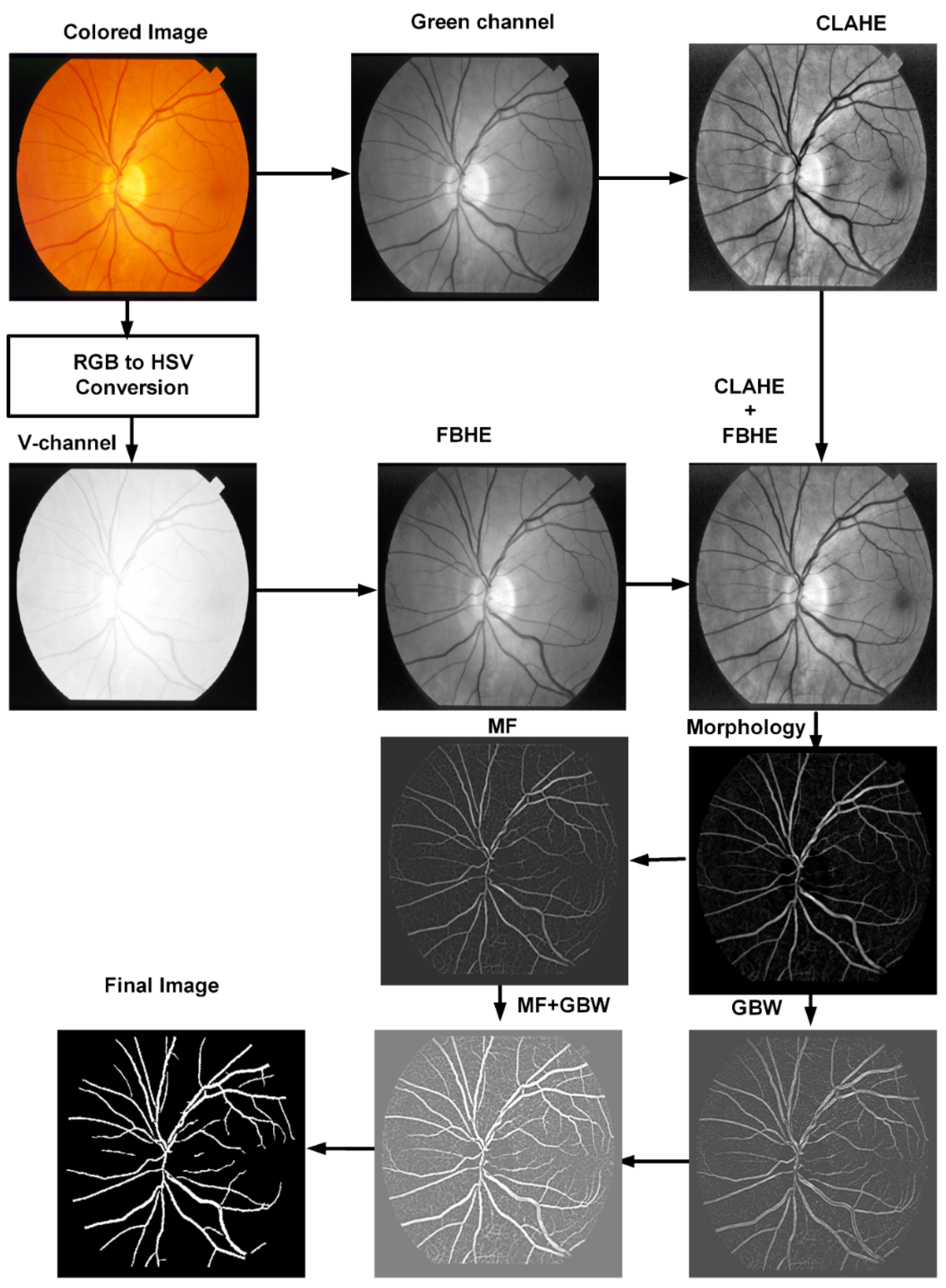
3. Materials and Methods

The suggested technique is applied on the two famous and most frequently used public benchmark datasets, the DRIVE [13] and STARE [14] datasets which contain colored images of retina.

Images from the DRIVE dataset were taken with the help of a Canon CR5 camera in the Netherland with a forty five degrees Field of View (FOV). The DRIVE dataset comprises of forty images (in which seven images contain pathology) and contains the manual segmentation of vessels as well. The sizes of the images are 768 × 584, eight bit per color channel whereas their FOV is 540 pixels in diameter approximately. The format of these pictures is Joint Photographic Experts Group (JPEG). These forty images have been subdivided into two sets, which are train and test set, where twenty images are there in each. The training set has three images that contain pathology while the testing set consists of four images containing pathology. The images in the DRIVE dataset are segmented through two observers manually. The training images of the dataset have one manual segmentation, while the testing images have two. The STARE dataset comprises twenty digitized images, which were captured by a Top Con TRV-50 fundus camera with thirty five degrees FOV. These images have a 605 × 700 pixels resolution. The FOV of the images is almost equal to 650 × 550 pixels diameter. In twenty images, ten images contain pathologies. These images were manually segmented according to two observers. In this regard, the first observer segmented the pixels of vessels in a percentage of 10.4 while the second observer segmented the pixels of vessels in a percentage of 14.9.

The overall block diagram of our suggested work has been described in Figure 1. In pre-processing, the morphological operators are required to eradicate the noise and to expand and enhance the contrast of an image. The color retinal images usually consist of non-uniform illumination problems, contrast variation and various types of structural abnormalities. Because of these factors achieving better segmentation becomes a very challenging task. These issues can be tackled by applying a proper preprocessing step. After pre-processing, we applied MF and Gabor wavelet filters for blood vessels segmentation. HVS is used to binarize the resultant image which is then post-processed to get the final image.

3.1. Preprocessing

In the preprocessing stage of the proposed method, two techniques are applied in parallel for improvement of the image contrast. The first is “fuzzy logic-based histogram equalization (FBHE)” [15] and second is “contrast limited adaptive histogram equalization (CLAHE)”. To apply FBHE, the RGB image is converted to the color space of HSV. In which V component is extended and stretched through conserving the chromatic information like Hue (H) as well as Saturation (S). Such approach is implied exclusively for improving the low contrast along with low bright regions in the color images. Here in, stretching of the component ‘V’ is implemented considering the effect of the enhancement parameters average intensity value ‘M’, where ‘K’ is the degree to which ‘V’ is intensified. This stretching will exactly transform the value ‘x’ for current intensity into the improved intensity value ‘Xe’. The parameter ‘M’ splits the intensities into two classes. For the first class, the Xe_c1 can be computed as given in Equation (1).

$$X{e}_{c1}=X+{\mu }_{D1}\left(x\right)K$$

(1)

For the second class, the Xe_c2 can be computed as given in Equation (2).

$$X{e}_{c2}=\left(X{\mu }_{D2}\left(x\right)\right)+\left(E-{\mu }_{D2}\left(x\right)K\right))$$

(2)

here,

$${\mu }_{D1}=\frac{1-\left(M-X\right)}{M}$$

(3)

$${\mu }_{D2}=\frac{E-X}{E-M}$$

(4)

where ‘E’ is the maximum possible value of intensity, and μ_D1 and μ_D2 are fuzzy membership values of class one and class two respectively. Details can be found at [15]. The image after enhancing using FBHE is shown in the middle of the second row, Figure 1.

In the second step of preprocessing, we have applied CLAHE [16] to expand the contrast of green channel from color fundus images. In green channel, red objects such blood vessels are well-contrasted. In CLAHE, the images are subdivided into contextual regions along with histograms on each of which contextual region are computed locally. On elevated peaks of the histogram, clipping is done as it shows noise. After that, histogram specification is applied on contextual regions. The CLAHE enhanced image is obtained and then bilinear interpolation is utilized to combine the individually enhanced histograms. The level of clipping determines the noise level considered to be smoothened and the contrast level intended to be increased in the histogram. The resulting image after applying CLAHE is shown in the first row last column of Figure 1. Images obtained after applying FBHE and CLAHE are added and scaled by a factor of 0.5, the resulting image is shown in the last column second row of Figure 1. It can be noticed that vessels are well-contrasted now.

3.2. Morphological Filter

Morphological filters are very effective in removing low-frequency noise and geometrical objects. In mathematical morphology, image is considered as a set, and the desired objects can be extracted by probing the image with another set of a known shape. This probing shape is known as the structuring element. Herein, the morphological filters can be applied on binary image as well as on grayscale image. The structuring element can have different shapes and sizes depending on the objects to be extracted. The various morphological operators include dilate, erode, open and close. They are used to perform different functions such as to remove image region boundary pixels. We used the top-hat morphological filter with a disc shape element on grayscale image to remove objects such ROI boundary. For a grayscale image I, it is defined as:

Top hat transform = I − (IoB)

(5)

where, IoB represents the image (I) opening with structuring element B. The selection of B is based on the shapes of the objects to be detected, in our case, these are round objects. The opening operation removes all the objects of interest from the image. Subtracting an opened image from the original image (top-hat transform) will result into removing all other objects and retains only the objects of interest. In this way using top-hat transform, we can keep all the objects of interest based on their shape or morphology.

The top-hat morphological filter used in this proposed work has a disc-shape element so that circular region boundaries such as the region of interest (ROI) boundary and the optic disc boundary can be removed. Details can be found in [17]. The image obtained after the application of the morphological filter is shown in the third row, right most column of Figure 1.

3.3. Matched Filter

Chaudhuri et al. [3] for the first time used match filter (MF) for detecting blood vessels. The cross-section of the blood vessel resembles Gaussian function. It produces a high response to the vessels and a low response for the background of nearly constant intensity. Mathematically, it is possible to express MF as

f(x,y) = −exp(−x^2/(2σ^2)); ∀|y| ≤ L/2

(6)

In Equation (6), L denotes the length of the section for which a fixed orientation is assumed for the vessel. And ‘σ’ refers to the width of vessel to be detected. Response produced by the MF will be high when kernel and vessels are in the same direction. Otherwise, for non-vessel, a relatively low response value is shown. In a non-ideal setting, the above technique reduces the probability of false detection of blood vessels. Blood vessels are located in different orientations in retinal fundus images. Therefore, to detect blood vessels in different orientations, the f(x,y) kernel should be rotated in different directions. It is rotated in 12 (at 15°) directions in the proposed method since the vessels can be oriented in any direction. The parameter values used in the proposed research are σ = 2 and L = 4.

3.4. Gabor Wavelet

A Gabor wavelet, Gabor kernel, Gabor filter or Gabor function represents the product for elliptical Gaussian envelope as well as a complex plane wave. Gabor [18] found that Gaussian-modulated complex exponentials realize the best trade-off among time and frequency resolutions, similar to Heisenberg’s uncertainty principle in physics. For 2D signals, mathematically it can be defined by:

$${\psi }_{\overline{k}}\left(\overline{x}\right)=\frac{\left|\left|\overline{k}\right|\right|}{{\sigma }^2}{e}^{\frac{{\left|\left|\overline{k}\right|\right|}^2{\left|\left|\overline{x}\right|\right|}^2}{2{\sigma }^2}}\left[e^{j\overline{k}\overline{x}}-e^{\frac{{\sigma }^2}{2}}\right]$$

(7)

where, $\overline{k}$ being the frequency vector defines the scale and direction of Gabor functions. $\overline{k}=k_v{e}^{j{\varphi }_O}$ and $k_v=\frac{\pi }{2f^v}$. $v$ is the scale of the wavelet, and $f$ is the spacing factor between kernels in frequency space. ${\varphi }_O=\frac{\pi O}{8},O=0,1,2,3\dots ,$. While $\overline{x}=\left(x,y\right)$ is the spatial domain variable. Thus, using 2D Gabor functions, we can enhance vessels and remove noise as they are directional and have the ability of tuning to specific frequencies [2]. In the proposed research work, we use single scale ($v=2$) of Gabor functions as we are also using a matched filter in parallel to the Gabor filter. We are using ten orientations, i.e., $O=0,1,2,3,\mathrm{..9}$, while $f$ = 2^0.5 and σ = π/3. Hence, ten Gabor wavelet kernels are produced, and the image is filtered using these kernels which results in 10 images. In each image thus obtained, square absolute values are calculated for each pixel and the resulting images are added to obtain a single image denoted by I_sum. Similarly, the real parts of those 10 images are also added together to obtain another image called I_sumR. Finally the Gabor-filtered image ($Ga{b}_I\left(x,y\right))$ is obtained by adding I_sum with I_sumR. The whole process is mathematically described according to the subsequent equation.

$$Ga{b}_I\left(x,y\right)=({\displaystyle \sum }_{O=0}^9{\left|\mathrm{I}\left(x,y\right)\ast {\psi }_{2,O}\left(x,y\right)\right|}^2){}^{1/2}+({\displaystyle \sum }_{O=0}^9\mathrm{real}\left(\mathrm{I}\left(x,y\right)\ast {\psi }_{2,O}\left(x,y\right)\right))$$

(8)

3.5. Human Visual System Based Binarization

To binarize the enhanced image, shown in Figure 1, last row middle image, the OFF-center surround method is used. This method is inspired from human visual system (HVS) [19,20] and was originally tested for document binarization and produced better results for constraints like shadows, varying illumination, noise, smear, along with strain degradations in the image. The ability to percept brightness from darkness in HVS is promoted based on two distinct cell populations for antagonistic responses, which are ON and OFF [19,20] center ganglion cells. Stimulations of the OFF cells is done based upon light decrements (by using dark stimuli across bright background) as is the case of blood vessel segmentation. The OFF center surround cells have two different sizes in order to respond to small and large stimuli. At least, the surround size has to be wide like the width of the thickest vessel in our case. First, the image is preprocessed pixel by pixel as described by the following equation so as to make the pixel value 0–255:

$${O^{\prime }}_{i,j}=\frac{O_{i,j}-O_{min}}{O_{max}-O_{min}}\times 255$$

(9)

where O_min represents the minimum for the original image O, O_max indicates its maximum, in addition to ${O^{\prime }}_{i,j}$ that denotes the preprocessed pixel.

$$Surroun{d}_{ij}^K=\frac{1}{{\left(2S^K+1\right)}^2}{\displaystyle \sum }_{y=1S^K}^{i+s^K}{\displaystyle \sum }_{x=j{S}^K}^{j+S^K}{O^{\prime }}_{i,j}$$

(10)

$$Cente{r}_{ij}^K=\frac{1}{{\left(2C^K+1\right)}^2}{\displaystyle \sum }_{y=1C^K}^{i+C^K}{\displaystyle \sum }_{x=j{C}^K}^{j+C^K}{O^{\prime }}_{y,x}$$

(11)

$$\begin{gathered} K=\left\{S,L\right\}S:L:large \\ {S}^K>C^K\forall K,S^S<S^L \end{gathered}$$

(12)

$$Surroun{d}_{i,j}=\frac{W{S}^s·Surroun{d}_{i,j}^S+W{S}^L·Surroun{d}_{i,j}^L}{W{C}^S+W{C}^L}$$

(13)

$$Cente{r}_{i,j}=\frac{W{C}^s·Cente{r}_{i,j}^S+W{C}^L·Cente{r}_{i,j}^L}{W{C}^S+W{C}^L}$$

(14)

$$S{C}_{i,j}=Surroun{d}_{i,j}-Cente{r}_{i,j}$$

(15)

$$G_{i,j}=\{\begin{array}{c}\frac{\left(255+Surroun{d}_{i,j}\right)·S{C}_{i,j}}{Surroun{d}_{i,j}+C{S}_{i,j}}\forall S{C}_{i,j}>0\\ 0\forall S{C}_{i,j}\le 0\end{array}$$

(16)

$Surroun{d}_{ij}^K$ and $Cente{r}_{ij}^K$ are defined as the mean intensity of image O′ at (i, j) position for the square areas, respectively from both surround and center, based on scale of K. K refers the scale for center-surround cell and S_K and C_K the sizes for both surround and center in K scale, respectively. Here,$W{S}^s$, $W{S}^L$ represent the weights for the surround values, $W{C}^s$, $W{C}^L$, represent the weights for the center values. Further details can be found at [5]. After binarization, the image is postprocessed which consists of merging three pixels apart objects and length filtering to remove objects which are 100 pixels or less.

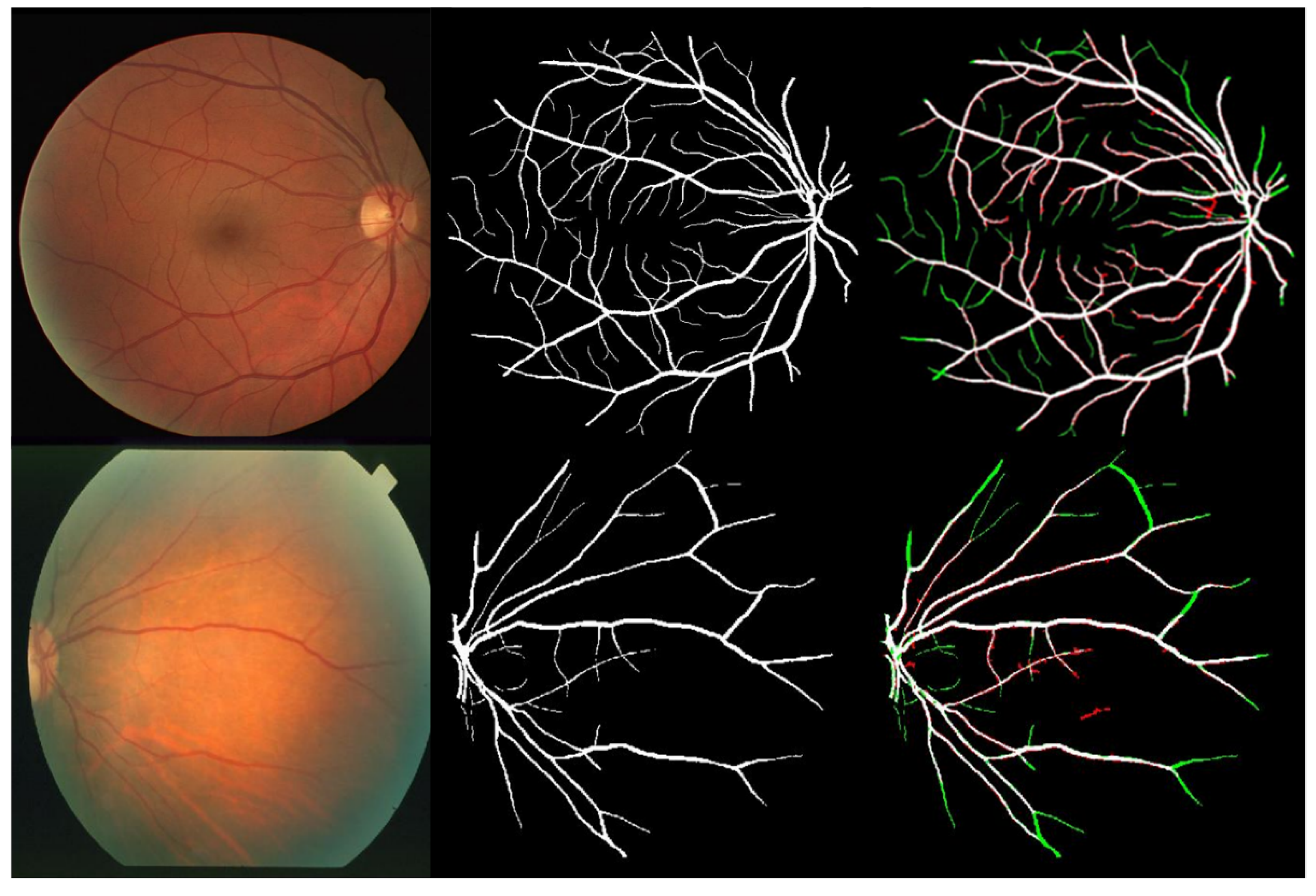
4. Results and Discussion

The performance given by the suggested system is assessed with regard to 1) sensitivity (Sen), 2) specificity (Spe) and 3) accuracy (Acc). These terms are mathematically defined in Equations (17)–(19), based on True-Positives (TP), True-Negatives (TN), False-Positives (FP), and False-Negatives (FP) are described in

Table 1. Definitions of TP, TN, FP, and FN.

TP	a pixel decided by the proposed system as vessel pixel, and it represents also vessel pixel according to ground truth
TN	a pixel decided by the proposed system as nonvessel pixel, and it is also non vessel pixel according to ground truth
FP	a pixel decided by the proposed system as vessel pixel, but it is non vessel pixel according to ground truth
FN	a pixel decided by the proposed system as non vessel pixel, but it represents vessel pixel according to ground truth

.

Sen = TP/(TP + FN)

(17)

Spe = 1 − TN/(TN + FP)

(18)

Acc = (TP + TN)/(TP + TN + FP + FN)

(19)

The unoptimized parameter values of HVS are given in

Table 2. Unoptimized values of HVS params.

Scale $\mathit{k}$	Surround Size, ${\mathit{S}}^{\mathit{k}}$	Center Size, ${\mathit{C}}^{\mathit{k}}$	$\mathit{W}{\mathit{S}}^{\mathit{K}}$	$\mathit{W}{\mathit{C}}^{\mathit{K}}$
$k$ = S, short	7	0	33	25
$k$ = L, large	9	3	90	75

.

The strength and weaknesses of proposed algorithm is found using images of the both above mentioned datasets. For the DRIVE dataset, separate images for training and testing are provided which are a set of 20 images each while in the case of the STARE dataset only 20 images are there. So there is no subdivision of dataset between train and test. Hence, similar to [21], we have used the first five images to estimate parameters of the proposed algorithm. In testing, all the 20 images from STARE dataset are used as described in

Table 3. Results of suggested technique.

DRIVE				STARE
Image No.	Sen	Spe	Acc	Sen	Spe	Acc
1.	0.7797	0.9755	0.9579	0.5861	0.9715	0.9405
2.	0.7564	0.9825	0.9592	0.5115	0.9737	0.9427
3.	0.6944	0.9825	0.9536	0.7331	0.9617	0.9479
4.	0.6894	0.9874	0.9598	0.6490	0.9814	0.9566
5.	0.6795	0.9872	0.9581	0.6882	0.9826	0.9558
6.	0.6594	0.9865	0.9545	0.8365	0.9714	0.9620
7.	0.6976	0.9857	0.9592	0.8078	0.9681	0.9552
8.	0.7068	0.9759	0.9525	0.7920	0.9716	0.9582
9.	0.6949	0.9834	0.9599	0.8085	0.9707	0.9579
10.	0.7308	0.9816	0.9608	0.7373	0.9774	0.9579
11.	0.6877	0.9825	0.9559	0.7728	0.9767	0.9621
12.	0.7718	0.9737	0.9561	0.8483	0.9749	0.9650
13.	0.7028	0.9789	0.9517	0.7370	0.9752	0.9539
14.	0.7958	0.9728	0.9584	0.6646	0.9798	0.9511
15.	0.7506	0.9775	0.9612	0.6784	0.9803	0.9541
16.	0.7358	0.9781	0.9560	0.6051	0.9831	0.9442
17.	0.6797	0.9798	0.9542	0.7540	0.9828	0.9622
18.	0.7443	0.9756	0.9571	0.7206	0.9888	0.9751
19.	0.8303	0.9745	0.9624	0.7663	0.9775	0.9684
20.	0.7543	0.9735	0.9573	0.6305	0.9716	0.9486
Mean	0.7271	0.9798	0.9573	0.7164	0.9760	0.9560

. The image-by-image results of the proposed algorithm are presented in Table 3, where the first three columns are for the DRIVE dataset and the last three columns are for the STARE dataset. On DRIVE dataset, the mean values for sensitivity (Sen), specificity (Spe) and accuracy (Acc) are 0.7272, 0.9798, and 0.9573 respectively. The maximum values obtained were 0.8303, 0.9874, and 0.9624 for Sen, Sep, and Acc, respectively. Similarly, For the STARE dataset, the mean values obtained were 0.7164, 0.9760, and 0.9560 for Sen, Spe, and Acc, respectively. The maximum values obtained were 0.8483, 0.9888, and 0.9751 for Sen, Spe, and Acc, respectively. Shown in Figure 2 are the best-case accuracies obtained on the DRIVE (first row) and STARE benchmark datasets (second row). The third column in Figure 2 illustrates the segmented images using the proposed algorithm. White pixels are the true vessel pixels, while the red are false positives and green represent missed vessel pixels. It can be noticed that the proposed method is good at segmenting the thick vessel very accurately, having very few false positives along the thick vessel edges. Figure 3, describes the worst-case accuracies obtained on DRIVE (first row) and STARE benchmark (second row) datasets. By observing Figure 3, it can be noted that the suggested technique has missed many fine vessel pixels. The thick vessels are still detected more precisely and clearly with very few false positives detected along their edges. In addition, there are negligible numbers of false positive pixels due to the region of interest (ROI) boundary and optic disc region, as can be observed both in the best-case and the worst-case accuracies, shown in Figure 2 and Figure 3, respectively. By careful observation of Figure 2 and Figure 3, it can be noticed that the suggested method is not able to segment many fine blood vessels. Also in case of fine vessels, there are false positives near their edges. Thus limitation of the suggested approach is the accurate detection for the fine vessel. A comparison of our algorithm with the current state-of-the-art approaches is presented in

Table 4. Performance comparison of proposed method with other state-of-the-art methods.

Dataset	DRIVE				STARE
Method/First Author	Year	Acc	Sen	Spe	Acc	Sen	Spe
Supervised
Thangaraj [22]	2018	0.9606	0.8014	0.9753	0.9435	0.8339	0.9536
Zhang [23]	2019	0.9544	0.8175	0.9767	0.9656	0.8068	0.9838
Tang [24]	2020	0.9477	0.7338	0.9730	0.9498	0.7518	0.9734
Adapa [25]	2020	0.9450	0.6994	0.9811	0.9486	0.6298	0.9839
Sayed [26]	2021	0.958	0.786	0.973	0.953	0.831	0.9630
Deep Learning
Yan [27]	2018	0.9542	0.7653	0.9818	0.9612	0.7581	0.9846
Soomro [28]	2018	0.9480	0.739	0.956	0.947	0.748	0.9620
Jiang [29]	2018	0.9624	0.7540	0.9825	0.9734	0.8352	0.9846
Alom [30]	2018	0.9556	0.7792	0.9813	0.9712	0.8298	0.9862
Khan [31]	2020	0.9649	0.8252	0.9787	-	-	-
Wu [32]	2020	0.9582	0.7996	0.9813	0.9672	0.7963	0.9863
Sathananthavathi [33]	2021	0.9577	0.7918	0.9708	0.9445	0.8021	0.9561
Unsupervised
Biswal [34]	2018	0.9500	0.7100	0.9700	0.9500	0.7000	0.9700
Pal [35]	2019	0.9431	0.6129	0.9744	-	-	-
Sundaram [36]	2019	0.9300	0.6900	0.9400	-	-	-
Khawaja [37]	2019	0.9553	0.8043	0.9730	0.9545	0.8011	0.9694
Upadhyay [38]	2020	0.9560	0.7890	0.9720	0.9610	0.7360	0.9810
Palanivel [39]	2020	0.9480	0.7375	0.9788	0.9542	0.7484	0.9780
Pachade [40]	2020	0.9552	0.7738	0.9721	0.9543	0.7769	0.9688
Tian [41]	2021	0.9554	0.6942	0.9802	0.9492	0.7019	0.9771
Mardani [42]	2021	0.9519	0.7667	0.9692	0.9524	0.7969	0.9664
Proposed Method	2022	0.9573	0.7271	0.9798	0.9560	0.7164	0.9760

with respect to of Acc, Sen, and Spe on DRIVE and STARE benchmark datasets.

In Table 4, it can be observed that the suggested technique has demonstrated a similar performance as state-of-the-art approaches including supervised or unsupervised algorithms with respect to accuracy. Furthermore, as expected, most of the deep learning-based approaches performed better than the proposed method. In the unsupervised category on the DRIVE dataset, the proposed algorithm realizes an accuracy of 0.9573, which is the best amongst all the methods described under the unsupervised category in Table 4. Similarly, we achieved an accuracy of 0.9560 on the STARE dataset, which is the second highest (the highest being the method of Upadhyay et al. [38]). Additionally, among the unsupervised category, the proposed system achieves the second highest specificity after Tian et al.’s method [41]. However, with the sensitivity of 0.7 or more the proposed system has the highest specificity among all the methods described under supervised and unsupervised categories on the DRIVE dataset, as shown in Table 4. To summarize, deep learning methods have performed much better with regard to Sen, Spe and Acc as compared to conventional methods both supervised and unsupervised. The deep learning method given in [29] reports the best results for both the DRIVE and STARE datasets. These are 0.9624, 0.7540 and 0.9825 for DRIVE and 0.973, 0.8352 and 0.9846 for STARE respectively, for Acc, Sen and Spe. However, these high values are obtained at a cost of the high computational requirement by a deep learning algorithm. Similarly, in conventional methods (other than deep learning), supervised approaches realize better performance than unsupervised approaches. For example, the best results in terms of Acc, Sen and Spe, reported in [22], are 0.9606, 0.8014 and 0.9753, respectively, on the DRIVE dataset. While, on the STARE dataset, 0.9656, 0.8068 and 0.9838 are obtained for Acc, Sen and Spe, respectively, reported in [23]. On the other side, supervised methods require intense training which necessitates computational resources and time.

Table 5. Execution time comparison.

DRIV			STARE
Method	System Specs	Acc	T in sec	Acc	T in sec
Thangaraj [22]	360 GHz Intel Core i7 20 GB RAM	0.9606	156	0.9435	203
Adapa [25]	2 * Intel Xeon E2620 v4, 64 GB RAM, Nvidia Tesla K40 GPU	0.9450	9	0.9486	9
Alom [30]	GPU machine besides 56 G of RAM and an NIVIDIA GEFORCE GTX-980 Ti.	0.9556	2.84	0.9712	6.42
Sathananthavathi [33]	Intel Core i5, 32 GB RAM	0.9577	10	0.9445	10
Biswal [34]	Intel core i3, 1.7 GHZ, 4 GBRAM	0.9500	3.3	0.9500	3.3
Khawaja [37]	Core i7, 2.21 GHz, 16 GB RAM	0.9553	5	0.9545	5
Palanivel [39]	2.9 GHz, 64 GB RAM	0.9480	60	0.9542	60
Pachade [40]	Intel Xenon, 2.00 GHz,16 GB RAM	0.9552	3.47	0.9543	6.10
Proposed Method	Intel(R) Xeon(R) 3.50GHz, 32 GB RAM.	0.9573	3.17	0.9560	3.17

presents the execution time comparison. It is not possible to exactly judge the performance of the systems based on execution time as the systems have different hardware specification and software used. But it gives some clue about the execution time requirements. It is vivid from the Table 5 that the proposed system is comparatively better than many of the entries in the table based on execution time and accuracy.

The diseases such as hypertension and diabetes can be diagnosed at early stage, through the identification of variations in the retinal blood vessels. The accurate segmentation of blood vessels helps to provide such information to ophthalmologists for better disease characterization [43]. Our method has shown promising results for large to medium size blood vessel segmentation similar to state-of-the-art methods.

5. Conclusions

Analysis of fundus images is vital in diagnosing various diseases whose symptoms appear in the retina of patients. One of the symptoms is the thickening of retinal blood vessels which can be studied through medical image analysis techniques like one proposed in this paper. In this work, we have suggested an unsupervised blood vessel segmentation method using color fundus images. Color fundus images normally suffer from varying and low contrast. To overcome this problem, we pre-processed the color fundus images using CLAHE and FBHE. Furthermore, we enhanced elongated objects using the tophat transform and extract the candidate blood vessel pixels using matched filtering and Gabor wavelet and finally obtained the blood vessel using the human visual system. The proposed system is assessed using two public benchmark datasets named DRIVE and STARE. The obtained mean values Sen, Spe and Acc are 0.7271, 0.9798, 0.9573 and 0.7164, 0.9760, 0.9560, respectively, for the DRIVE and STARE datasets. These measures are similar to current state-of-the-art methods albeit at a smaller computational requirement of 3.17 s.

References

1. Shah, S.A.A.; Laude, A.; Faye, I.; Tang, T.B. Automated microaneurysm detection in diabetic retinopathy using curvelet transform. J. Biomed. Opt. 2016, 21, 101404. [Google Scholar] [CrossRef] [PubMed] [Green Version]
2. Schwartz, R.; Dodge, J.; Smith, N.A.; Etzioni, O. Green ai. Commun. ACM 2020, 63, 54–63. [Google Scholar] [CrossRef]
3. Chaudhuri, S.; Chatterjee, S.; Katz, N.; Nelson, M.; Goldbaum, M. Detection of blood vessels in retinal images using two-dimensional matched filters. IEEE Trans. Med. Imaging 1989, 8, 263–269. [Google Scholar] [CrossRef] [PubMed] [Green Version]
4. Soares, J.V.; Leandro, J.J.; Cesar, R.M.; Jelinek, H.F.; Cree, M.J. Retinal vessel segmentation using the 2-D Gabor wavelet and supervised classification. IEEE Trans. Med. Imaging 2006, 25, 1214–1222. [Google Scholar] [CrossRef] [PubMed] [Green Version]
5. Vonikakis, V.; Andreadis, I.; Papamarkos, N. Robust document binarization with OFF center-surround cells. Pattern Anal. Appl. 2011, 14, 219–234. [Google Scholar] [CrossRef]
6. Shah, S.A.A.; Tang, T.B.; Faye, I.; Laude, A. Blood vessel segmentation in color fundus images based on regional and Hessian features. Graefe’s Arch. Clin. Exp. Ophthalmol. 2017, 255, 1525–1533. [Google Scholar] [CrossRef]
7. Al-Rawi, M.; Karajeh, H. Genetic algorithm matched filter optimization for automated detection of blood vessels from digital retinal images. Comput. Methods Programs Biomed. 2007, 87, 248–253. [Google Scholar] [CrossRef]
8. Cinsdikici, M.G.; Aydın, D. Detection of blood vessels in ophthalmoscope images using MF/ant (matched filter/ant colony) algorithm. Comput. Methods Programs Biomed. 2009, 96, 85–95. [Google Scholar] [CrossRef]
9. Zhang, B.; Zhang, L.; Zhang, L.; Karray, F. Retinal vessel extraction by matched filter with first-order derivative of Gaussian. Comput. Biol. Med. 2010, 40, 438–445. [Google Scholar] [CrossRef] [Green Version]
10. Li, Q.; You, J.; Zhang, D. Vessel segmentation and width estimation in retinal images using multiscale production of matched filter responses. Expert Syst. Appl. 2012, 39, 7600–7610. [Google Scholar] [CrossRef]
11. Oliveira, W.S.; Teixeira, J.V.; Ren, T.I.; Cavalcanti, G.D.; Sijbers, J. Unsupervised retinal vessel segmentation using combined filters. PLoS ONE 2016, 11, e0149943. [Google Scholar] [CrossRef] [PubMed] [Green Version]
12. Saroj, S.K.; Kumar, R.; Singh, N.P. Fréchet PDF based Matched Filter Approach for Retinal Blood Vessels Segmentation. Comput. Methods Programs Biomed. 2020, 194, 105490. [Google Scholar] [CrossRef] [PubMed]
13. Staal, J.; Abràmoff, M.D.; Niemeijer, M.; Viergever, M.A.; Van Ginneken, B. Ridge-based vessel segmentation in color images of the retina. IEEE Trans. Med. Imaging 2004, 23, 501–509. [Google Scholar] [CrossRef] [PubMed]
14. Hoover, A.; Kouznetsova, V.; Goldbaum, M. Locating blood vessels in retinal images by piecewise threshold probing of a matched filter response. IEEE Trans. Med. Imaging 2000, 19, 203–210. [Google Scholar] [CrossRef] [PubMed] [Green Version]
15. Raju, G.; Nair, M.S. A fast and efficient color image enhancement method based on fuzzy-logic and histogram. AEU-Int. J. Electron. Commun. 2014, 68, 237–243. [Google Scholar] [CrossRef]
16. Zuiderveld, K. Contrast limited adaptive histogram equalization. Graph. Gems 1994, 474–485. [Google Scholar]
17. Haralick, R.M.; Sternberg, S.R.; Zhuang, X. Image analysis using mathematical morphology. IEEE Trans. Pattern Anal. Mach. Intell. 1987, 4, 532–550. [Google Scholar] [CrossRef]
18. Gabor, D. Theory of communication. Part 1: The analysis of information. J. Inst. Electr. Eng.-Part III Radio Commun. Eng. 1946, 93, 429–441. [Google Scholar] [CrossRef] [Green Version]
19. Nelson, R.; Kolb, H. ON and OFF pathways in the vertebrate retina and visual system. Vis. Neurosci. 2004, 1, 260–278. [Google Scholar]
20. Werner, J.S.; Chalupa, L.M. The Visual Neurosciences; Mit Press: Cambridge, MA, USA, 2004. [Google Scholar]
21. Shah, S.A.A.; Shahzad, A.; Khan, M.A.; Lu, C.K.; Tang, T.B. Unsupervised method for retinal vessel segmentation based on gabor wavelet and multiscale line detector. IEEE Access 2019, 7, 167221–167228. [Google Scholar] [CrossRef]
22. Thangaraj, S.; Periyasamy, V.; Balaji, R. Retinal vessel segmentation using neural network. IET Image Processing 2018, 12, 669–678. [Google Scholar] [CrossRef]
23. Sai, Z.; Yanping, L. Retinal Vascular Image Segmentation Based on Improved HED Network. Acta Optica Sinica 2020, 40, 0610002. [Google Scholar]
24. Tang, S.; Yu, F. Construction and verification of retinal vessel segmentation algorithm for color fundus image under BP neural network model. J. Supercomput. 2021, 77, 3870–3884. [Google Scholar] [CrossRef]
25. Adapa, D.; Joseph Raj, A.N.; Alisetti, S.N.; Zhuang, Z.; Naik, G. A supervised blood vessel segmentation technique for digital Fundus images using Zernike Moment based features. PLoS ONE 2020, 15, e0229831. [Google Scholar] [CrossRef]
26. Sayed, M.A.; Saha, S.; Rahaman, G.A.; Ghosh, T.K.; Kanagasingam, Y. An innovate approach for retinal blood vessel segmentation using mixture of supervised and unsupervised methods. IET Image Processing 2021, 15, 180–190. [Google Scholar] [CrossRef]
27. Yan, Z.; Yang, X.; Cheng, K.-T. Joint segment-level and pixel-wise losses for deep learning based retinal vessel segmentation. IEEE Trans. Biomed. Eng. 2018, 65, 1912–1923. [Google Scholar] [CrossRef]
28. Soomro, T.A.; Afifi, A.J.; Gao, J.; Hellwich, O.; Paul, M.; Zheng, L. Strided U-Net model: Retinal vessels segmentation using dice loss. In Proceedings of the 2018 Digital Image Computing: Techniques and Applications (DICTA), Canberra, Australia, 10–13 December 2018. [Google Scholar]
29. Jiang, Z.; Zhang, H.; Wang, Y.; Ko, S.B. Retinal blood vessel segmentation using fully convolutional network with transfer learning. Comput. Med. Imaging Graph. 2018, 68, 1–15. [Google Scholar] [CrossRef]
30. Alom, M.Z.; Hasan, M.; Yakopcic, C.; Taha, T.M.; Asari, V.K. Recurrent residual convolutional neural network based on u-net (r2u-net) for medical image segmentation. arXiv 2018, arXiv:1802.06955. [Google Scholar]
31. Khan, T.M.; Alhussein, M.; Aurangzeb, K.; Arsalan, M.; Naqvi, S.S.; Nawaz, S.J. Residual connection-based encoder decoder network (RCED-Net) for retinal vessel segmentation. IEEE Access 2020, 8, 131257–131272. [Google Scholar] [CrossRef]
32. Wu, Y.; Xia, Y.; Song, Y.; Zhang, Y.; Cai, W. NFN+: A novel network followed network for retinal vessel segmentation. Neural Netw. 2020, 126, 153–162. [Google Scholar] [CrossRef]
33. Sathananthavathi, V.; Indumathi, G. Encoder enhanced atrous (EEA) unet architecture for retinal blood vessel segmentation. Cogn. Syst. Res. 2021, 67, 84–95. [Google Scholar]
34. Biswal, B.; Pooja, T.; Subrahmanyam, N.B. Robust retinal blood vessel segmentation using line detectors with multiple masks. IET Image Processing 2018, 12, 389–399. [Google Scholar] [CrossRef]
35. Wu, Y.; Xia, Y.; Song, Y.; Zhang, Y.; Cai, W. Morphological operations with iterative rotation of structuring elements for segmentation of retinal vessel structures. Multidimens. Syst. Signal Processing 2019, 30, 373–389. [Google Scholar]
36. Sundaram, R.; Ks, R.; Jayaraman, P. Extraction of blood vessels in fundus images of retina through hybrid segmentation approach. Mathematics 2019, 7, 169. [Google Scholar] [CrossRef] [Green Version]
37. Khawaja, A.; Khan, T.M.; Khan, M.A.; Nawaz, S.J. A multi-scale directional line detector for retinal vessel segmentation. Sensors 2019, 19, 4949. [Google Scholar] [CrossRef] [Green Version]
38. Upadhyay, K.; Agrawal, M.; Vashist, P. Unsupervised multiscale retinal blood vessel segmentation using fundus images. IET Image Processing 2020, 14, 2616–2625. [Google Scholar] [CrossRef]
39. Palanivel, D.A.; Natarajan, S.; Gopalakrishnan, S. Retinal vessel segmentation using multifractal characterization. Appl. Soft Comput. 2020, 94, 106439. [Google Scholar] [CrossRef]
40. Pachade, S.; Porwal, P.; Kokare, M.; Giancardo, L.; Meriaudeau, F. Retinal vasculature segmentation and measurement framework for color fundus and SLO images. Biocybern. Biomed. Eng. 2020, 40, 865–900. [Google Scholar] [CrossRef]
41. Tian, F.; Li, Y.; Wang, J.; Chen, W. Blood Vessel Segmentation of Fundus Retinal Images Based on Improved Frangi and Mathematical Morphology. Comput. Math. Methods Med. 2021. [Google Scholar] [CrossRef]
42. Mardani, K.; Maghooli, K. Enhancing retinal blood vessel segmentation in medical images using combined segmentation modes extracted by DBSCAN and morphological reconstruction. Biomed. Signal Processing Control 2021, 69, 102837. [Google Scholar] [CrossRef]
43. Nguyen, T.T.; Wang, J.J.; Wong, T.Y. Retinal vascular changes in pre-diabetes and prehypertension: New findings and their research and clinical implications. Diabetes Care 2007, 30, 2708–2715. [Google Scholar] [CrossRef] [PubMed] [Green Version]
Figure 1. Block diagram of the suggested algorithm.
Applsci 12 06393 g001
Figure 2. Best case accuracy: First column represents color images, second ground truth and third segmented images. First row contains DRIVE images, and STARE images are there in the second row. Last column: white indicate the pixels of true positives; while the green pixels denote the missed vessel pixels, whereas red are false positives.
Applsci 12 06393 g002
Figure 3. Worst case accuracy: First column indicate color images, second ground truth and third segmented images. First row contains DRIVE images and STARE images are there in the second row. Last column, white indicate the pixels of true positives; while green pixels denote the missed vessel pixels, whereas red refer false positives.
Applsci 12 06393 g003