Scale-Adaptive Deep Matching Network for Constrained Image Splicing Detection and Localization

Abstract

Constrained image splicing detection and localization (CISDL) is a newly formulated image forensics task that aims at detecting and localizing the source and forged regions from a series of input suspected image pairs. In this work, we propose a novel Scale-Adaptive Deep Matching (SADM) network for CISDL, consisting of a feature extractor, a scale-adaptive correlation module and a novel mask generator. The feature extractor is built on VGG, which has been reconstructed with atrous convolution. In the scale-adaptive correlation computation module, squeeze-and-excitation (SE) blocks and truncation operations are integrated to process arbitrary-sized images. In the mask generator, an attention-based separable convolutional block is designed to reconstruct richer spatial information and generate more accurate localization results with less parameters and computation burden. Last but not least, we design a pyramid framework of SADM to capture multiscale details, which can increase the detection and localization accuracy of multiscale regions and boundaries. Extensive experiments demonstrate the effectiveness of SADM and the pyramid framework.

1. Introduction

With the widespread availability of affordable acquisition devices such as smartphones and the easy use of powerful image editing software, we can easily modify digital images without leaving any perceptible artifacts [1]. Malicious tampered images can distort the truth in news reports, or destroy someone’s reputation and privacy, leading to potentially devastating consequences [2]. Digital image forensics intends to verify the authenticity of digital images and provide automatic tools to detect image manipulation [3]. In conventional image forensics methods, image manipulation always causes high-level or low-level inconsistencies, which can determine whether images have been tampered with. However, these image forensics techniques only investigate a single image, and the information provided by the single image is limited [1,4,5]. So, it is difficult to identify fake images accurately with the improved image editing techniques. Otherwise, these conventional image forensics methods do not provide the source of the forged area or the specific tampering process, which reduces the persuasion of the detection results in practical application.

To tackle these limitations, constrained image splicing detection and localization (CISDL) was proposed to find forged regions and corresponding source regions in a pair of candidate images by comparing pixel-level features [6,7]. Theoretically, with a probe image P and a potential donor image D, CISDL aims to determine whether P has spliced regions from D. In [6], Wu et al. designed a deep matching and validation network (DMVN) for CISDL. It contains four modules: a feature extractor, an inception-based mask deconvolution module, a visual consistency validator module and a Siameselike module. DMVN is the first method to address CISDL task and uses visual comparison to show the localization performance. In [8], Ye et al. proposed a feature pyramid deep matching and localization network (FPLN), which can detect and localize small spliced regions by fusing pyramidal feature maps with different resolution [1]. However, the loss of spatial information limits the discriminative ability and localization accuracy of the splicing model. In [7], Liu et al. proposed a new deep matching network for CISDL named DMAC, using atrous convolution to generate two high-quality candidate masks. Additionally, they employ a detection network and a discriminative network to optimize the pretrained DMAC further. Though this framework achieves remarkable improvement than DMVN, the discriminative ability of DMAC and DMVN for simple scalar product is still limited in correlation computation. Liu et al. proposed an encoder–decoder architecture based on an attention-aware mechanism in [9], which is named as AttentionDM to mitigate these problems. AttentionDM generates fine-grained masks by building a decoder with atrous spatial pyramid pooling (ASPP) [10]. A channel attention block is added to the correlation computation module to emphasize channelwise informative features. However, AttentionDM can only process fixed-size images for the restriction of correlation computation module and cannot be applied to actual multiscale target detection. In a word, there are still some challenges hindering the development of CISDL: (1) fixed-size image processing; (2) degraded spatial information of extracted features; (3) multiscale objects.

In this paper, we propose a novel Scale-Adaptive Deep Matching network (SADM), as shown in Figure 1. In the proposed method, we make three improvements: First, a scale-adaptive correlation computation module is proposed based on squeeze-and-excitation (SE) blocks [11] and truncation operations to deal with arbitrary-sized images. Second, an attention-based separable convolutional block is constructed in mask generator to recover spatial information further. The attention-based separable convolutional block is composed of depthwise separable convolution and spatial attention, that depthwise separable convolution can help to improve efficiency as well as reduce the model parameters. Meanwhile, spatial attention can help recover the spatial information. Last but not least, we propose a pyramid framework of SADM to address the problem of insufficient edge detection and multiscale object detection.

In summary, our contributions are:

–

A novel scale-adaptive deep matching network (SADM) is constructed based on a newly designed scale-adaptive correlation computation module.

–

A novel mask generator is designed by attention-based separable convolutional blocks, consisting of depthwise separable convolution and spatial attention. This kind of hybridized combination is helpful for spatial information reconstruction with low computational complexity.

–

A pyramid framework of SADM (PSADM) is proposed to process the multiscale objects.

–

Extensive experiments prove the excellent performance of SADM and PSADM.

This paper is organized as follows. Section 2 describes the related work. Section 3 introduces SADM and the pyramid version of SADM. Experimental results and visual comparisons are presented in Section 4. In Section 5, we make a conlusion.

2. Related Work

2.1. Image Forensics

Digital image forensics [12,13] has two main tasks: image forgery localization and detection. The purpose of image forgery detection is to determine whether an image has been forged, while image forgery localization is to mark the forged area on the forged image. The main primary of tampering detection technology is that the statistical features inherently in digital image acquisition are inevitably disturbed by tampering operations. That manipulated images can be detected and distinguished by analyzing these features. In practical image forensics applications, users are concerned more about which areas of the image rather than whether an image has been tampered with, making tampering localization an important research topic in image forensics.

In recent years, deep learning algorithms [14,15,16] represented by convolutional neural networks [17,18,19], recurrent neural networks [20] and generative adversarial networks have been widely used in many fields such as image classification [21,22], object detection [23], semantic segmentation [24,25], image retrieval [26], scene understanding [27], etc. and have made a leap forward compared with traditional methods. Given the outstanding performance of deep learning algorithms in computer vision, researchers have also tried to adopt deep learning algorithms to solve some problems in image forensics. However, in terms of tampering localization, both traditional methods and the recent emergence of deep learning feature-based methods are still difficult to achieve industrial application [28]. In this work, we focus on the visual features of tampered images and the statistical inconsistency between pixels to investigate the image tampering localization. Besides, we also try to explore effective and robust image tampering localization methods by using deep learning algorithms for homologous and heterologous tampering.

2.2. CISDL

Constrained image splicing detection and localization, proposed for image forensic task, plays a crucial part in constructing a germline genesis map of an image by dense matching. This task aims to afford the source image of the tampered region and the corresponding region by finding high similarity of corresponding regions over long distances. Studying CISDL has great display significance in improving the accuracy of image stitching detection and localization, etc. The three methods to address this task are as follows: Wu et al. first proposed a method to address CISDL specifically [6]. They apply a deep convolutional neural network architecture to deep matching and validation network (DMVN) with two input images. DMVN is composed of a feature extractor with convolutional neural network (CNN), a inception-based mask deconvolution module, a visual consistency validator module and a siameselike module producing a probability value. The value indicates the likelihood between donor image and query image, as for the spliced region. Yet, in [6], it explained the localization performance by visual comparison and didn’t evaluate quantitatively. And DMVN also performs poorly in detecting accurate boundaries and small regions for comparing with high-level resolution feature maps of VGG [10] merely. Liu et al. then proposed a novel framework for CISDL with adversarial learning [7]. The proposed framework contains a deep matching network based on atrous convolution (DMAC), a detection network and a discriminative network. The detection network and the discriminative network can optimize the masks generated from DMAC adversarially. Compared to DMVN, the DMAC network accomplishes real-time behavior in a scene with a large crowd of manipulated images by fully end-to-end architecture. Instead of the adversarial learning framework of DMAC, Liu et al. proposed an attention-aware deep matching network for CISDL, named AttentionDM [9]. Overall, AttentionDM employs an encoder–decoder architecture to generate fine-grained masks. AttentionDM contains a feature extractor by employing VGG16 with atrous convolution, an attention-aware correlation computation module and mask generator module with ASPP blocks to generate the fine-grained mask. Significant progress has been made that the DMVN network has sufficient ability to detect small tampered areas and locate the edges of tampered areas. However, both DMAC and AttentionDM are sensitive to changes in image size and can only manufacture fixed images. Besides, many researched images are uncorrelated or unforged in the actual application, which all cause serious problems. In a sense, when combining the query and donor images, a spliced image can be rendered as a copy-move detection task. So, when CISDL was first proposed, Wu et al. compared against baseline algorithms from the state-of-the-art copy-move detection algorithms and used precision, recall and F1-score to detect spliced image correctly [6]. Besides, Ref. [29] also applies DMVN to judge whether an image has copy-move regions: they feed DMVN the pair of (X1, X2), which is split along X’s longer axis. And they judge the X contains copy-move regions (one in X1 and the other in X2) by whether DMVN finds a splice. If not, they then split X1 and X2 into halves again. Above all, constrained image splicing detection and localization methods are mutually linked to copy-move detection method.

3. Method

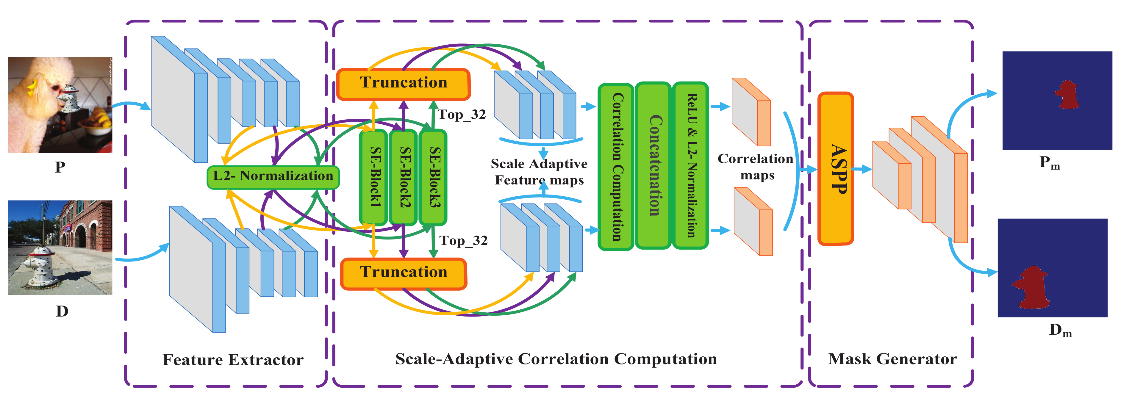
Our method has three components: the feature extractor, the scale-adaptive correlation computation module and the mask generator. The feature extractor employs VGG16, but removes the maxpooling operation while using atrous convolution in the last convolutional block. In Figure 1, from the feature extractor, three feature maps are generated with the same size. The scale-adaptive correlation computation module adopts SE blocks and truncation operations to break the limit of image size. The mask generator designs an attention-based separable convolutional block based on depthwise separable convolution and spatial attention. Depthwise separable convolution can effectively improve the deep matching, and spatial attention can restore spatial information. In terms of the overall structure, we employ channel attention first, learning ‘what’ in the channel axes, and spatial attention second, learning ‘where’ in the spatial axes, for which can blend cross-channel and spatial information [30]. Additionally, the pyramid version of SADM is proposed to make full use of multiscale information to improve the ability of multiscale objects location.

3.1. Feature Extractor with Atrous Convolution

The structure and parameter settings of the feature extractor, a transformed version of VGG16, are shown in Figure 2. Our feature extractor consists of five blocks. The first two blocks contain two convolutional layers and one maxpooling operation, respectively. The third block includes three convolutional layers and one maxpooling operation. To generate three feature maps of the same size, only three convolutional layers are used in the last two blocks without maxpooling operation. In general, three points differ from VGG16:

(1)

Removing maxpooling operations in the fourth and fifth convolutional blocks. This change makes the final size of the feature map from $W/32$ × $H/32$ to $W/8$ × $H/8$ and upgrades image resolution [10].

(2)

Adding atrous convolution at the fifth block of VGG16 [10]. Atrous convolution generalizes standard convolution operation, which utilizes the numerical value of parameters to control the resolution of the feature map for freedom. Specifically, by adjusting the filter’s field-of-view, atrous convolution can collect multiscale information. Atrous convolution is calculated as:

$$y(i_c,j_c)=\sum _{k_1,k_2}w(k_1,k_2)\times x(i_c+r_c{k}_1,j_c+r_c{k}_2)$$

(1)

where y(i${}_c$, j${}_c$) denotes the output of the atrous convolution of a 2-D input of signal x($i_c$, $i_c$). Besides, $k_1$, $k_2$ ∈ [$-f$l($\frac{K}{2}$),fl($\frac{K}{2}$)], w($k_1$, $k_2$) denotes a K × K filter, atrous rate $r_c$ means the sampling stride of the input signal. And the atrous of fifth block is set with $r_c$ = 2.

(3)

Skip architecture. Due to removing the maxpooling operation of VGG16’s last two blocks [10], F${}_{\mathit{n}}^{\left(1\right)}$ and F${}_n^{\left(2\right)}$ (n ∈ {3, 4, 5}) are produced with the same size. A high-level feature contains rich semantic information, while a low-level feature contains detailed spatial information. Next, F${}_3^{\left(k\right)}$, F${}_4^{\left(k\right)}$, F${}_5^{\left(k\right)}$ (k ∈ {1, 2}) are fed into the scale-adaptive correlation computation module and the mask generator.

3.2. Scale-Adaptive Correlation Computation

As for previous studies, they can not handle arbitrary-sized images. Such as the process of matching response using cross-correlation in DMVN, it uses all pixels of the feature map relative to the size of the image. Similarly, DMAC and AttentionDM continued to use this approach. So, they are all restricted by the size of images. Therefore, distinctly accounting for image scale is essential for improving the model’s ability to process low-resolution and high-resolution images.

In order to address this defect, Liu et al. proposed a sliding window-based matching strategy to process high-resolution images, but it causes high computational complexity [9]. In this paper, we employ correlation computation with SE blocks and truncation operations to boost our model’s ability to process arbitrary-sized images. F${}_3^{\left(k\right)}$, F${}_4^{\left(k\right)}$, F${}_5^{\left(k\right)}$ (k ∈ {1, 2}) are extracted from the feature extractor, and then each feature map has to go through the L2-normalization, SE blocks and truncation operations. At last, we utilize ReLU and L2-normalization to produce the final two correlation maps.

(1)

SE blocks

For each channel of the convolution feature, SE blocks model their interdependencies explicitly. Specifically, SE blocks take each channel of feature map as a feature detector, then they utilize global information to emphasize informative features or suppress unuseful ones selectively. Before the SE blocks, L2-normalization is conducted:

$${\overline{\overrightarrow{f}}}^{\left(k\right)}(i_k,j_k)=\frac{{\overrightarrow{f}}^{\left(k\right)}(i_k,j_k)}{\Vert {\overrightarrow{f}}^{\left(k\right)}(i_k,j_k){\Vert }_2}$$

(2)

where F${}^{\left(k\right)}$ ∈ $\mathbb{R}$${}^h$${}^{\times }$${}^w$${}^{\times }$${}^c$, k ∈{1, 2}, ${\overrightarrow{f}}^{\left(1\right)}$($i_1$, $j_1$) ∈ F${}^{\left(1\right)}$, ${\overrightarrow{f}}^{\left(2\right)}$($i_2$, $j_2$) ∈ F${}^{\left(2\right)}$. And then, we can get two feature maps after standardization, $\overline{\mathbf{F}}$${}^{\left(1\right)}$, $\overline{\mathbf{F}}$${}^{\left(2\right)}$. Next, SE blocks are applied to recalibrate informative features, making an improvement on discriminating features. Based on these above, our SE block has three steps: First, using global average pooling to exploit contextual information. We denote z${}^{\left(k\right)}$ ∈ $\mathbb{R}$${}^C$ as channelwise statistics, and denote $\overrightarrow{f}$${}^{\left(k\right)}$ as homologous channel dimensions feature, H × W, the cth element of z${}^{\left(k\right)}$ is computed with:

$${\displaystyle z_c^{\left(k\right)}={\mathbf{F}}_{sq}\left({\overline{\overrightarrow{f}}}_c^{\left(k\right)}\right)=\frac{1}{H\times W}\sum _{i=1}^H\sum _{j=1}^W{\overline{\overrightarrow{f}}}_c^{\left(k\right)}(i,j)}$$

(3)

This operation, global average pooling, is the simplest aggregation technique to collect local descriptors that can express the whole image. The second step is to capture channelwise dependencies, which consists of a ReLU and a sigmoid activation as a gating mechanism:

$$\mathbf{s}={\mathbf{F}}_{ex}({\mathbf{z}}^{\left(k\right)},\mathbf{W})=\sigma ({\mathbf{W}}_2\delta \left({\mathbf{W}}_1\left({\mathbf{z}}^{\left(k\right)}\right)\right)$$

(4)

where $\delta$ refers to the ReLU function, W${}_1$ ∈ $\mathbb{R}$${}^{\frac{C}{r}\times C}$ and W${}_2$ ∈ $\mathbb{R}$${}^C$${}^{\times }$${}^{\frac{C}{r}}$. The third step is to weight the characteristics of each channel, with the weight obtained above. The final output is computed with:

$${\ddot{\mathbf{F}}}^{\left(k\right)}={\mathbf{F}}_{scale}({\overline{\overrightarrow{f}}}_c^{\left(k\right)},s_c)$$

(5)

where ${\ddot{\mathbf{F}}}^{\left(k\right)}$ = [$\ddot{\overrightarrow{f}}$${}_1^{\left(k\right)}$,$\ddot{\overrightarrow{f}}$${}_2^{\left(k\right)}$,⋯, $\ddot{\overrightarrow{f}}$${}_c^{\left(k\right)}$] and F${}_{scale}$(${\overline{\overrightarrow{f}}}_c^{\left(k\right)}$) indicate the channelwise multiplication between the scalar s${}_c$ and the feature map ${\overline{\overrightarrow{f}}}^{\left(k\right)}$ ∈ $\mathbb{R}$${}^H$${}^{\times }$${}^W$.

(2)

Correlation-computation with truncation operations

The process of this part is shown in Figure 3. $\ddot{\mathbf{F}}$${}^{\left(1\right)}$ and $\ddot{\mathbf{F}}$${}^{\left(2\right)}$ refer to the feature maps computed from the SE blocks, $\ddot{\overrightarrow{f}}$${}^{\left(1\right)}$($i_1$, $j_1$) ∈ $\ddot{\mathbf{F}}$${}^{\left(1\right)}$, $\ddot{\overrightarrow{f}}$${}^{\left(2\right)}$($i_2$, $j_2$) ∈ $\ddot{\mathbf{F}}$${}^{\left(2\right)}$. The correlation maps are computed by:

$${\mathbf{C}}^{\left(12\right)}(i_{12},j_{12},m_{12})={\ddot{\overrightarrow{f}}}^{\left(1\right)}{(i_1,j_1)}^T{\ddot{\overrightarrow{f}}}^{\left(2\right)}(i_2,j_2)$$

(6)

where C${}^{\left(12\right)}$ is obtained by comparing $\ddot{\overrightarrow{f}}$${}^{\left(1\right)}$($i_1$, $j_1$) ∈ $\ddot{\mathbf{F}}$${}^{\left(1\right)}$ and $\ddot{\overrightarrow{f}}$${}^{\left(2\right)}$($i_2$, $j_2$) ∈ $\ddot{\mathbf{F}}$${}^{\left(2\right)}$. Since the corresponding ${\ddot{\overrightarrow{f}}}^{\left(1\right)}{(i_1,j_1)}^T$ are not known in advance and most fraction of the features are irrelative, we sort the C${}^{\left(12\right)}$($i_{12}$, $j_{12}$, $m_{12}$) along the (h × w) channels, and select top-T values:

$${\widehat{\mathbf{C}}}^{\left(12\right)}(i_{12},j_{12},1:T)=\mathrm{Top}\_\mathrm{T}\left(\mathrm{Sort}\left({\mathbf{C}}^{\left(12\right)}({\mathrm{i}}_{12},{\mathrm{j}}_{12},:)\right)\right)$$

(7)

If apply a curve to show $\widehat{\mathbf{C}}$${}^{\left(12\right)}$($i_{12}$, $j_{12}$), it is supposed to be a monotonic decreasing curve. Once an abrupt drop appeared, it means $\widehat{\mathbf{C}}$${}^{\left(12\right)}$($i_{12}$, $j_{12}$) has matched regions. So, the T channels should include the most drops. Due to the operation of the top-T selection, our network was given the capability of accepting arbitrary-sized images. We summarize above correlation computation as:

$${\widehat{\mathbf{C}}}^{\left(12\right)}=\mathrm{Corr}({\ddot{\mathbf{F}}}^{\left(1\right)},{\ddot{\mathbf{F}}}^{\left(2\right)})$$

(8)

This is an example of handling a correlation map between two feature maps. After input F${}_3^{\left(k\right)}$, F${}_4^{\left(k\right)}$, F${}_5^{\left(k\right)}$, the scale-adaptive correlation computation module procedure can be concluded as Algorithm 1.

Algorithm 1: Scale-Adaptive Correlation Computation

Require: Image $\mathbf{I}$${}^{\left(1\right)}$ and $\mathbf{I}$${}^{\left(2\right)}$

1: “Hierarchical features extraction:”

2: ${\mathbf{F}}_3^{\left(1\right)}$, F${}_4^{\left(1\right)}$, F${}_5^{\left(1\right)}$= Encoder($\mathbf{I}$${}^{\left(1\right)}$)

3: ${\mathbf{F}}_3^{\left(2\right)}$, F${}_4^{\left(2\right)}$, F${}_5^{\left(2\right)}$= Encoder($\mathbf{I}$${}^{\left(2\right)}$)

4: “Attention weighted feature maps generation for hierarchical features:”

5: for c = 3 to 5 do

6:  “L2 normalization of Equation (2)”

7:  ${\overline{\mathbf{F}}}_n^{\left(1\right)}$ = L2_norm(F${}_n^{\left(1\right)}$)

8:  ${\overline{\mathbf{F}}}_n^{\left(2\right)}$ = L2_norm(F${}_n^{\left(2\right)}$)

9:  “Refer to Equations (3)–(5)”

10:  ${\ddot{\mathbf{F}}}_n^{\left(1\right)}$ = ${\mathbf{F}}_{scale}({\overline{\mathbf{F}}}_m^{\left(1\right)},{\mathbf{F}}_{sq}({\overrightarrow{f}}_c^{\left(1\right)})$

11:  ${\ddot{\mathbf{F}}}_n^{\left(2\right)}$ = ${\mathbf{F}}_{scale}({\overline{\mathbf{F}}}_n^{\left(2\right)},{\mathbf{F}}_{sq}({\overrightarrow{f}}_c^{\left(2\right)})$

12: end for

13: “Correlation computation based on hierarchical attention weighted feature maps:”

14: for c = 3 to 5 do

15:  “Refer to Equation (8) based on Equations (6) and (7)”

16:  ${\widehat{\mathbf{C}}}_n^{\left(12\right)}$ = $\mathrm{Corr}({\ddot{\mathbf{F}}}_n^{\left(1\right)},{\ddot{\mathbf{F}}}_n^{\left(2\right)})$

17:  ${\widehat{\mathbf{C}}}_n^{\left(11\right)}$ = $\mathrm{Corr}({\ddot{\mathbf{F}}}_n^{\left(1\right)},{\ddot{\mathbf{F}}}_n^{\left(1\right)})$

18:  ${\widehat{\mathbf{C}}}_n^{\left(21\right)}$ = $\mathrm{Corr}({\ddot{\mathbf{F}}}_n^{\left(2\right)},{\ddot{\mathbf{F}}}_n^{\left(1\right)})$

19:  ${\widehat{\mathbf{C}}}_n^{\left(22\right)}$ = $\mathrm{Corr}({\ddot{\mathbf{F}}}_n^{\left(2\right)},{\ddot{\mathbf{F}}}_n^{\left(2\right)})$

20:  “Concatenate correlation maps”

21:  ${\mathbf{C}}_n^{\left(1\right)}$ = $\{{\widehat{\mathbf{C}}}_n^{\left(12\right)},{\widehat{\mathbf{C}}}_n^{\left(11\right)}\}$

22:  ${\mathbf{C}}_n^{\left(2\right)}$ = $\{{\widehat{\mathbf{C}}}_n^{\left(21\right)},{\widehat{\mathbf{C}}}_n^{\left(22\right)}\}$

23: end for

24: “Concatenate hierarchical correlation maps”

25: ${\mathbf{C}}^{\left(1\right)}=\{{\mathbf{C}}_3^{\left(1\right)},{\mathbf{C}}_4^{\left(1\right)},{\mathbf{C}}_5^{\left(1\right)}\}$

26: ${\mathbf{C}}^{\left(2\right)}=\{{\mathbf{C}}_3^{\left(2\right)},{\mathbf{C}}_4^{\left(2\right)},{\mathbf{C}}_5^{\left(2\right)}\}$

27: “ReLU and L2 normalization”

28: ${\overline{\mathbf{C}}}^{\left(1\right)}=\mathrm{L2\_norm}(\max ({\mathbf{C}}^{\left(1\right)},0))$

29: ${\overline{\mathbf{C}}}^{\left(2\right)}=\mathrm{L2\_norm}(\max ({\mathbf{C}}^{\left(2\right)},0))$

Ensure: Correlation maps ${\overline{\mathbf{C}}}^{\left(1\right)}$ and ${\overline{\mathbf{C}}}^{\left(2\right)}$ of ${\mathbf{I}}^{\left(1\right)}$ and ${\mathbf{I}}^{\left(2\right)}$

In Algorithm 1, each group of the feature map, extracted from the same layer of feature extractor, will through the operation of L2-normalization and SE blocks. And then, for each two feature maps from the same layer, we utilize correlation computation and truncation operations to get two pairs of correlation maps, i.e., ${\overline{\mathbf{C}}}_n^{\left(12\right)}$, ${\overline{\mathbf{C}}}_n^{\left(11\right)}$ and ${\overline{\mathbf{C}}}_n^{\left(21\right)}$, ${\overline{\mathbf{C}}}_n^{\left(22\right)}$ are produced from ${\ddot{\mathbf{F}}}_n^{\left(1\right)}$ and ${\ddot{\mathbf{F}}}_n^{\left(2\right)}$ (n ∈ {1, 2, 3}). Next, concatenating each group of correlation maps, we get two correlation maps, i.e., ${\mathbf{C}}_n^{\left(1\right)}$ and ${\mathbf{C}}_n^{\left(2\right)}$ (n ∈ {1, 2, 3}). Last, correlation maps $\mathbf{C}$${}^{\left(1\right)}$, $\mathbf{C}$${}^{\left(2\right)}$ are generated by concatenating ${\mathbf{C}}_n^{\left(1\right)}$ and ${\mathbf{C}}_n^{\left(2\right)}$ respectively. Since the associated areas should have the same symbol and should all be positive, we employ ReLU to convert negative values to zero. And then apply L2-normalization to access the normalized correlation maps as ${\overline{\mathbf{C}}}^{\left(1\right)}$, ${\overline{\mathbf{C}}}^{\left(2\right)}$. Next, the process of handling these correlation maps will be shown in the next section.

3.3. Mask Generator Based on Attention-Based Separable Convolutional Module

Our mask generator integrates ASPP blocks, maxpooling layers and attention-based separable convolutional blocks to generate high-resolution masks. The architecture and parameter settings are shown in Figure 4. It consists of an ASPP block, three upsampling layers, three attention-based separable convolutional blocks and a 1 × 1 convolution to reduce channels at last. Additionally, each attention-based separable convolutional block is followed by an L2-normalization layer.

Briefly, ASPP contains several atrous convolution for conducting multiscale objects. As shown in Figure 5, the attention-based separable convolutional block is applied to generate fine-grained masks, including two layers of depthwise separable convolution and one layer of spatial attention. Depthwise separable convolution can improve the speed and accuracy for deep matching to locate and discriminate regions with less parameters and computation burden. Spatial attention can assign greater weights to critical sections so that the model can focus more attention on it. Qualitatively, this mask generator shows improvement in its ability to address spatial information problems as well as detect edges and small areas. And quantitatively, it reduces computational complexit with less model parameters. In summary, our SADM typically employs attention-based separable convolutional blocks to gain a good tradeoff between localization and detection performance and computation complexity.

(1)

ASPP.

Before the ASPP block, the correlation computation module produces a feature tensor of size $W/8$ × $H/8$ × 96. ASPP is the first part of the mask generator with three parallel layers of atrous convolution to capture multiscale features, setting atrous rates with [6, 12, 18]. Then the feature maps are concatened into a 1 × 1 convolution to reduce channels.

(2)

Attention-based separable convolutional block.

The mask generator uses attention-based separable convolutional block for three times, corresponding to the three times of upsampling operations. The design of attention-based separable convolutional block is shown in Figure 5. It employs depthwise separable convolution for two times first and a spatial attention second, utilizing L2-normalization, ReLU among them.

Depthwise separable convolution. The depthwise separable convolution is shown in Figure 6. Motivated by the architecture of [31], we adopt a variant of depthwise separable convolution for our mask generator. Different from ecumenical depthwise separable convolution, we utilize the 1 × 1 pointwise convolution followed by the 3 × 3 depthwise convolution for each input channel and concatenate into the subsequent layers. We apply it to mask generator to reduce the model parameters uttermost. Similar to the Xception network [31], we employ L2-normalization and ReLU between pointwise convolution and depthwise convolution.

Spatial attention. Spatial attention can capture the spatial dependencies and produce more powerful pixel-level characterization, helping recover the spatial detail information effectively. The detail of spatial attention is shown in Figure 6. Let P denote the feature map input to spatial attention blocks, P(i, j) denotes a c-dimensional descriptor at at (i, j). Noted that P ∈ $\mathbb{R}$${}^h$${}^{\times }$${}^w$${}^{\times }$${}^c$, i ∈ [1, h], j ∈ [1, w], h and w indicate the height and width of the feature map and h = w in our work. Prior to reinforce P using spatial attention, we employ L2-normalization and ReLU to modify it. Then, the first step is to transform P into two feature spaces by the 1 × 1 convolution layer, f(P) = PW${}_{\mathit{f}}$ + $\mathbf{b}$${}_{\mathit{f}}$ and g(P) = PW${}_{\mathit{g}}$ + $\mathbf{b}$${}_{\mathit{g}}$. The similarity between f(P) and each g(P) is calculated as follows:

$$s^{(x,y)}=\mathit{f}{\left({\mathbf{P}}^{\left(x\right)}\right)}^T\mathit{g}\left({\mathbf{P}}^{\left(y\right)}\right)$$

(9)

In order to normalize these weights, we use a softmax function:

$${\beta }^{(x,y)}=\frac{exp\left(s^{(x,y)}\right)}{{\sum }_{y}exp\left(s^{(x,y)}\right)}$$

(10)

when predicting the xth region, ${\beta }^{(x,y)}$ denotes the extent that the model attends to the yth location, x, y ∈ [1, h × w]. The final attention is implemented as a 1 × 1 convolutional layer and computed as:

$${\displaystyle {\mathbf{o}}^{\left(x\right)}=\sum _y{\beta }_{xy}\mathit{h}\left({\mathbf{P}}^{\left(y\right)}\right)}$$

(11)

In the above equation, $\mathit{h}\left(\mathbf{P}\right)=\mathbf{P}{\mathbf{W}}_{\mathit{h}}+{\mathit{b}}_{\mathit{h}}$. And ${\mathbf{W}}_{\mathit{f}}\in {\mathbb{R}}^{c\times \frac{c}{8}}$, ${\mathbf{W}}_{\mathit{h}}\in {\mathbb{R}}^{c\times c}$, ${\mathbf{W}}_{\mathit{g}}$ ∈ $\mathbb{R}$${}^{c\times \frac{c}{8}}$, $\mathit{b}$${}_{\mathit{f}}$ ∈ $\mathbb{R}$${}^{\frac{c}{8}}$, $\mathit{b}$${}_{g,\mathit{h}}$ ∈ $\mathbb{R}$${}^{\frac{c}{8}}$, $\mathit{b}$${}_{\mathit{h}}$ ∈ $\mathbb{R}$${}^c$. After attention reinforced, the feature maps is calculated as:

$$\ddot{\mathbf{F}}=Atten\left(\mathbf{P}\right)=\lambda \mathit{O}+\mathbf{P}$$

(12)

where $\mathit{O}$ = {$\mathit{o}$${}^{\left(1\right)}$, $\mathit{o}$${}^{\left(2\right)}$,⋯,$\mathit{o}$${}^{(h}$${}^{\times }$${}^{w)}$}, $\lambda$ represents a scale parameter that can be initialized as zero and gradually learn a proper value.

3.4. Pyramid Version of SADM

The localization of object boundaries is vital for tampering detection. Specially, when multiscale objects appear in the image, it will increases the probe sophistication of tampered regions. Score maps play a crucial role in the CISDL task as it can reliably predict the presence and rough positioning of objects. But, score maps are not sensitive to pinpointing the exact outline of the tampered area. In this regime, explicitly accounting for object boundaries across different scales makes an essential contribution to CISDL’s successful handling of large and small objects. There are two main types of study designs to solve multiscale objects prediction challenge. The first approach is to train the model on a dataset that adapts to certain types of transformations, such as shift, rotation, scale, luminance and deformation changes. By applying multiple parallel filters with different rates, the second approach is to harness ASPP to exploit multiscale features. These two approaches have displayed an excellent capacity to represent scale.

In this paper, we employ an alternative method, called the pyramid version of SADM (PSADM), to handle this problem. First, feeding multiple rescaled versions of the original image to parallel module branches with the same parameters. Second, every scale score maps are bilinear interpolated to the original image resolution, converting image classification networks into dense feature extractors without learning any additional parameters, making the training speed of CNN in practice faster. Bilinear interpolation requires two linear transformations, the first one on the X-axis:

$$f\left(M_1\right)=\frac{x_2-x}{x_2-x_1}f\left(M_{11}\right)-\frac{x-x_1}{x_2-x_1}f\left(N_{21}\right)$$

(13)

$$f\left(M_2\right)=\frac{x_2-x}{x_2-x_1}f\left(N_{12}\right)-\frac{x-x_1}{x_2-x_1}f\left(N_{22}\right)$$

(14)

where $M_1=(x,y_1)$, $M_2=(x,y_2)$, $N_{11}=(x_1,y_1)$, $N_{21}=(x_2,y_1)$, $N_{12}=(x_1,y_2)$, $N_{22}=(x_2,y_2)$. Then find the target point in the region by another linear transformation:

$$f(x,y)=\frac{y_2-y}{y_2-y_1}f\left(M_1\right)-\frac{y-y_1}{y_2-y_1}f\left(M_2\right)$$

(15)

Third, fuse them by taking the average response across scales for each position separately. Finally, a new score map is got. The discussion in the experimental section shows that the pyramid version with scale = {384, 512, 640} achieves the best performance.

4. Experiment

In this section, we demonstrate the superiority of our model from an experimental point of view. In the task of CISDL, the most challenging are (1) processing arbitrary-sized images; (2) finding spliced regions as well as pinpointing their exact boundaries under various transformations; and (3) processing the multiscale object in the same image. Based on the above challenges, the enhanced effect of the model on tampering area localization and detection was verified by visual comparisons and quantitative results for the three improvements.

4.1. Benchmark Datasets and Compared Methods

To evaluate the effectiveness of SADM and PSADM, we conducted localization and detection experiments of tampered regions. According to the characteristics of each dataset, we evaluate the localization performance on the generated dataset from MS COCO and verify that SADM outperforms all the previous approaches. Then, the paired CASIA dataset and Media Forensics Challenge 2018 (MFC2018) dataset are tested to demonstrate the superiority of the proposed model in terms of detection performance.

(1)

The generated datasets from MS COCO.

The MS COCO dataset consists of 82,783 training images and 40,504 testing images. It provides object annotations for abundant images and can generate accurate ground truth masks by the enormous number of training pairs, which is suitable for localization performance experiments. After synthesis of the MS COCO dataset, thethe generated dataset’s training sets consist of 1035,255 training pairs, of which one-third were foreground pairs, one-third were background pairs, and one-third were negative sample pairs. The generated dataset’s test sets were divided into three main groups, namely the Difficult set (1–10%), the Normal set (10–25%) and the Easy set (25–50%). We adopt the pixel-level IoU (Intersection over Union), NMM (Nimble Mask Metric) and MCC (Matthews Correlation Coefficient) of the tampered regions and the average indicator of all the tested image pairs to evaluate the localization performance.

(2)

The paired CASIA dataset.

The CASIA TIDEv2.0 dataset is initially designed for the image of copy-move and the classic splicing detection problem [6]. The new paired CASIA dataset we used consists of 3642 positive samples and 5000 negative samples selected from the CASIA TIDEv2.0 dataset by CISDL. Due to the lack of ground truth masks, this new paired CASIA dataset only focuses on estimating the splicing detection performance [6]. We adopt F1-score, precision and recall to evaluate the detection performance.

(3)

MFC2018.

The Media Forensics Challenge 2018 (MFC2018) dataset has 16,673 negative image pairs and 1327 positive image pairs. MFC2018 is a challenging dataset, collected particularly for two problems of the CISDL task: quantitative evaluation of detection performance and localization performance, using a large number of negative image pairs and ground truth by visual comparison. We use AUC, an official metric, to quantify the capability to distinguish between the two categories and employ the EER (Equal Error Rate) score to evaluate false-alarm images.

4.2. Training Procedure and Testing Set

This model is trained with a 1 × 10⁻⁶ base learning rate for 3 epochs and 18 samples for each batch size. To calculate the model loss, we use the BCEWithLogitsLoss function. Meanwhile, we employ the Adadelta optimizer to optimize model parameters. Additionally, our feature extractor uses a migration learning approach by using a pre-trained model of VGG16 [10]. Since the scale of objects in the image is arbitrary, a fixed size perceptual field will limit the localization and detection effect, and ability to recognize object boundaries. To address these problems, we use diverse groups of different scale images to find the best formal of our model. The scale of each input image is experimented with [384, 512, 640], [448, 512, 576], respectively, called as PSADM. We adopt postfix to annotate different strategies, such as “ [384, 512, 640]” denotes the rescaled version of original images, and the size of original images are identified by “256/384/512”.

Experiments demonstrate that the localization performance is improved to a new level after adopting this strategy.

4.3. Experimental Results

4.3.1. The Generated Datasets from MS COCO

(1)

Parametric test.

Truncation error. We adopted a truncation operation in the scale-adaptive correlation calculation module to process arbitrary-sized images. After sorting the response values for the feature maps generated from SE-blocks, we tested the response values for the first 32, 128 and 256 channels. The test results are shown in

Table 1. Truncation error of SADM.

Method	Diffcult			Normal			Easy
	IoU	MCC	NMM	IoU	MCC	NMM	IoU	MCC	NMM
SADM32-L2	0.7759	0.8128	0.5129	0.9040	0.8288	0.8265	0.9621	0.9616	0.9410
SADM128-L2	0.7649	0.8115	0.5057	0.8981	0.8260	0.8266	0.9450	0.9563	0.9452
SADM256-L2	0.7602	0.8240	0.4987	0.8937	0.8244	0.8166	0.9434	0.9488	0.9246

. The model has the best localization performance when the response values of the first 32 channels are taken. As the response value decreases, the feature it represents becomes weaker. Therefore taking too many of these response values is not conducive to feature extraction.

The comparision of L1-normalization and L2-normalization. Based on the determined parameters of the truncation operation, we tested the types of normalization used in the model, including L1-normalization and L2-normalization, as shown in

Table 2. The comparision of L1-Normalization an L2-Normalization.

Method	Diffcult			Normal			Easy
	IoU	MCC	NMM	IoU	MCC	NMM	IoU	MCC	NMM
SADM32-L1	0.7702	0.8340	0.5167	0.8937	0.9244	0.8166	0.9484	0.9688	0.9246
SADM32-L2	0.7759	0.8128	0.5129	0.9040	0.8288	0.8265	0.9621	0.9616	0.9410

. There is little difference in the localization effect between using L1-normalization and L2-normalization, with L2-normalization showing slightly better results. Combining the above two points, SADM indicates that the truncation operation takes the first 32 channels and uses L2-normalization in the subsequent article.

(2)

Localization performance.

Table 3. Localization performance comparison on the generated datasets from MS COCO of SADM and PSADM.

Method	Diffcult			Normal			Easy
	IoU	MCC	NMM	IoU	MCC	NMM	IoU	MCC	NMM
DMVN [6]	0.2722	0.3533	−0.4382	0.6818	0.7570	0.4042	0.8198	0.8544	0.6770
DMAC [7]	0.5114	0.6308	0.0335	0.8279	0.8815	0.6840	0.9222	0.9395	0.8685
DMAC-adv [7]	0.5433	0.6584	0.1026	0.8317	0.8833	0.6877	0.9237	0.9411	0.8655
AttentionDM [9]	0.7228	0.8108	0.4793	0.8980	0.9320	0.8253	0.9602	0.9603	0.9388
SADM	0.7759	0.8128	0.5129	0.9040	0.8288	0.8265	0.9621	0.9616	0.9410
SADM-384	0.7828	0.8442	0.5060	0.8991	0.9321	0.8401	0.9621	0.9707	0.9495
SADM-512	0.7829	0.8521	0.5857	0.9042	0.9223	0.9281	0.9625	0.9663	0.9552
PSADM-avg-[384, 512, 640]	0.8089	0.8746	0.6070	0.9247	0.9534	0.9403	0.9738	0.9908	0.9761
PSADM–avg-[448, 512, 576]	0.7863	0.8523	0.5859	0.9111	0.9361	0.9397	0.9626	0.9796	0.9588
PSADM-max-[384, 512, 640]	0.7931	0.8632	0.5961	0.8993	0.9569	0.9299	0.9829	0.9825	0.9632
PSADM-max-[448, 512, 576]	0.7849	0.8514	0.5793	0.8976	0.9347	0.9287	0.9598	0.9693	0.9605

shows the localization performance on the generated datasets. As for processing the image of 256 × 256, the SADM significantly improves localization capability compared with previous models such as AttentionDM. In [7], Liu et al. employed a sliding window strategy to compensate for the defect of only being able to handle fixed-size images. Yet, it consumes more computing time. To compare with the sliding window strategy, we evaluate the effectiveness of the scale-adaptive correlation computation module on the same dataset. The results of handling 256 × 256, 384 × 384, 512 × 512 are shown in Table 3. As we can see, it is obvious that IoU, MCC and NMM are rising, which thoroughly explains the strong ability of SADM to process arbitrary-sized images. To further improve the capability of processing large-scale images, many kinds of parameters of the PSADM have been experimented with, as shown in Table 3. Under various considerations, the PSADM-512-[384, 512, 640] achieves superior performance on recognizing small regions and pinpointing their exact outline. And then, we will test the detection ability of this version.

(3)

Complexity analyses.

Table 4. Time complexity analyses.

Method	Time/s	Parameters	Framework
DMVN [6]	0.2968	10,473,788	Keras/Theano
DMAC/DMAC-adv [7]	0.0288	14,920,520	PyTorch
AttentionDM [9]	0.0306	15,758,162	PyTorch
SADM	0.0298	15,407,276	PyTorch

lists the testing time, parameters numbers and implemented frameworks. All experiments were conducted on a machine with Intel(R) Core (TM) i7-5930K CPU @ 3.50 GHz, 64 GB RAM and a single GPU (TITAN X). As shown in Table 4, the number of the trainable parameters for SADM is 15,407,276, slightly more than the number of parameters for DMAC but less than AttentionDM. Although the testing time of SADM is 0.0298 s, marginally lower than that of DMAC, it achieves significant improvements in localization and detection.

4.3.2. The Paired CASIA Dataset

In [9], AttentionDM was compared with DMVN and DMAC. In the comparison on CASIA, the previous scores are from [9]. In this paper, we calculate the average score of the tampered area as the detection score (here called tampering probability). In other words, we calculate the average score of the detected regions with {s${}^{\left(k\right)}$|k = 1, 2} for each generated mask firstly. And then the mean value, (s${}^{\left(1\right)}$ + s${}^{\left(2\right)}$) / 2, is computed as the final forged probability. As shown in

Table 5. Comparisons on the paired CASIA dataset.

Method	Precision	Recall	F1-Score
Christlein et al. [32]	0.5164	0.8292	0.6364
Luo et al. [33]	0.9969	0.5353	0.6966
Ryu et al. [34]	0.9614	0.5859	0.7309
Cozzolino et al. [35]	0.9897	0.6334	0.7725
DMVN-loc [6]	0.9152	0.7918	0.8491
DMVN-det [6]	0.9415	0.7908	0.8596
DMAC [7]	0.9255	0.8668	0.8952
DMAC-adv [7]	0.9657	0.8576	0.9085
AttentionDM [9]	0.9288	0.9204	0.9246
SADM-256	0.9741	0.8758	0.9263
SADM-384	0.9835	0.8771	0.9314
SADM-512	0.9903	0.8778	0.9316
PSADM-512-[384, 512, 640]	0.9932	0.8924	0.9329

, SADM has a very high Precision (nearly 100%) and a little low Recall value. For the size of 256 × 256, SADM improves the precision from 92.88% to 99.01%, while the recall score only decreases by 3.87%. F1-score has been further improved, which is a good tradeoff between Precision and Recall. As for the large-size such as 512 × 512, these indicators are further enhanced. In addition, the detection performance of large-scale images is further enhanced by the processing of PSADM. Visual comparisons, afforded in Figure 7, show that SADM achieves very good performance. It has a high level of competence in detecting small regions and accurate boundaries. Furthermore, it is also sensitive to the arbitrary-sized images as well as robust to transformation and rotation changes.

4.3.3. MFC2018

Since MFC2018 is definitely collected for the CISDL task, we compare SADM, PSADM with DMVN, DMAC and AttentionDM on MFC2018. The MFC2018 challenge provides the evaluation codes, AUC and EER scores, which are calculated and shown in

Table 6. Comparisons on MFC2018.

Method	AUC	EER
DMAC [7]	0.7542	0.3123
DMAC-adv [7]	0.7511	0.3093
AttentionDM [9]	0.7922	0.2756
SADM-256	0.7782	0.2527
SADM-384	0.7825	0.2490
SADM-512	0.7945	0.2470
PSADM-512-[384, 512, 640]	0.7982	0.2489

[36]. Compared with AttentionDM [9], SADM achieves the lowest EER score for 256 × 256 images with an AUC decreased by 0.014, which far exceeded the previous CISDL approach. As for large-scale images, SADM can also achieve higher AUC and lower EER. Additionally, PSADM further enhance the effect of processing large-scale images, with AUC increased by 0.0037 and EER decreased by 0.0019 based on “SADM-512”. Figure 8 provides visual comparisons. Obviously, SADM has a better capability to detect small regions and accurate boundaries than previous methods.

5. Conclusions

In this paper, we propose a Scale-Adaptive Deep Matching network (SADM) for CISDL, and a pyramid version of SADM (PSADM). SADM consists of three components: the feature extractor, the scale-adaptive correlation computation module and the mask generator. The correlation-computation with truncation operations are proposed to deal with arbitrary-sized images. The mask generator is designed to reconstruct the spatial information of an image and generate fine-grained mask without requiring more computational complexity. The PSADM is applied to improve the ability of multiscale object detection and matching. Experimental results show that the proposed method can achieve better performance than the state-of-the-art methods on the publicly available datasets.

References

1. Li, C.; Ma, Q.; Xiao, L.; Li, M.; Zhang, A. Image splicing detection based on Markov features in QDCT domain. Neurocomputing 2017, 228, 29–36. [Google Scholar] [CrossRef]
2. Tang, W.; Li, B.; Tan, S.; Barni, M.; Huang, J. CNN-based adversarial embedding for image steganography. IEEE Trans. Inf. Forensics Secur. 2019, 14, 2074–2087. [Google Scholar] [CrossRef] [Green Version]
3. Matern, F.; Riess, C.; Stamminger, M. Gradient-based illumination description for image forgery detection. IEEE Trans. Inf. Forensics Secur. 2019, 15, 1303–1317. [Google Scholar] [CrossRef]
4. Cozzolino, D.; Verdoliva, L. Noiseprint: A CNN-Based Camera Model Fingerprint. IEEE Trans. Inf. Forensics Secur. 2020, 15, 144–159. [Google Scholar] [CrossRef] [Green Version]
5. Liu, Y.; Guan, Q.; Zhao, X.; Cao, Y. Image Forgery Localization Based on Multi-Scale Convolutional Neural Networks. In Proceedings of the 6th ACM Workshop on Information Hiding and Multimedia Security, Innsbruck, Austria, 20–22 June 2018; pp. 85–90. [Google Scholar]
6. Wu, Y.; Abd-Almageed, W.; Natarajan, P. Deep Matching and Validation Network: An End-to-End Solution to Constrained Image Splicing Localization and Detection. In Proceedings of the 25th ACM International Conference on Multimedia, Mountain View, CA, USA, 23–27 October 2017; pp. 1480–1502. [Google Scholar]
7. Liu, Y.; Zhu, X.; Zhao, X.; Cao, Y. Adversarial Learning for Constrained Image Splicing Detection and Localization Based on Atrous Convolution. IEEE Trans. Inf. Forensics Secur. 2019, 14, 2551–2566. [Google Scholar] [CrossRef]
8. Ye, K.; Dong, J.; Wang, W.; Peng, B.; Tan, T. Feature Pyramid Deep Matching and Localization Network for Image Forensics. In Proceedings of the 2018 Asia-Pacific Signal and Information Processing Association Annual Summit and Conference (APSIPA ASC), Honolulu, HI, USA, 12–15 November 2018; pp. 1796–1802. [Google Scholar] [CrossRef]
9. Liu, Y.; Zhao, X. Constrained Image Splicing Detection and Localization With Attention-Aware Encoder-Decoder and Atrous Convolution. IEEE Access 2020, 8, 6729–6741. [Google Scholar] [CrossRef]
10. Simonyan, K.; Zisserman, A. Very Deep Convolutional Networks for Large-Scale Image Recognition. arXiv 2015, arXiv:1409.1556. [Google Scholar]
11. Hu, J.; Shen, L.; Sun, G. Squeeze-and-Excitation Networks. In Proceedings of the 2018 IEEE/CVF Conference on Computer Vision and Pattern Recognition (CVPR), Salt Lake City, UT, USA, 18–23 June 2018; IEEE Computer Society: Los Alamitos, CA, USA, 2018; pp. 7132–7141. [Google Scholar] [CrossRef] [Green Version]
12. Zeng, H.; Kang, X.; Peng, A. A multi-purpose countermeasure against image anti-forensics using autoregressive model. Neurocomputing 2016, 189, 117–122. [Google Scholar] [CrossRef]
13. Xiao, D.; Wang, Y.; Xiang, T.; Bai, S. High-payload completely reversible data hiding in encrypted images by an interpolation technique. Frontiers Inf. Technol. Electron. Eng. 2017, 18, 1732–1743. [Google Scholar] [CrossRef]
14. Yang, F.; Zhang, W.; Tao, L.; Ma, J. Transfer Learning Strategies for Deep Learning-based PHM Algorithms. Appl. Sci. 2020, 10, 2361. [Google Scholar] [CrossRef] [Green Version]
15. Zhang, S.X.; Zhu, X.; Yang, C.; Wang, H.; Yin, X.C. Adaptive Boundary Proposal Network for Arbitrary Shape Text Detection. In Proceedings of the IEEE/CVF International Conference on Computer Vision (ICCV), Montreal, QC, Canada, 10–17 October 2021; pp. 1305–1314. [Google Scholar]
16. Li, C.; Wei, F.; Dong, W.; Wang, X.; Yan, J.; Zhu, X.; Liu, Q.; Zhang, X. Spatially Regularized Streaming Sensor Selection. In Proceedings of the Thirtieth AAAI Conference on Artificial Intelligence, Phoenix, AZ, USA, 12–17 February 2016; pp. 3871–3879. [Google Scholar]
17. Miah, A.S.M.; Shin, J.; Hasan, M.A.M.; Rahim, M.A. BenSignNet: Bengali Sign Language Alphabet Recognition Using Concatenated Segmentation and Convolutional Neural Network. Appl. Sci. 2022, 12, 3933. [Google Scholar] [CrossRef]
18. Alshowaish, H.; Al-Ohali, Y.; Al-Nafjan, A. Trademark Image Similarity Detection Using Convolutional Neural Network. Appl. Sci. 2022, 12, 1752. [Google Scholar] [CrossRef]
19. Zhu, X.; Li, Z.; Lou, J.; Shen, Q. Video super-resolution based on a spatio-temporal matching network. Pattern Recognit. 2021, 110, 107619. [Google Scholar] [CrossRef]
20. Nam, J.; Kang, J. Classification of Chaotic Signals of the Recurrence Matrix Using a Convolutional Neural Network and Verification through the Lyapunov Exponent. Appl. Sci. 2021, 11, 77. [Google Scholar] [CrossRef]
21. Li, C.; Zhen, T.; Li, Z. Image Classification of Pests with Residual Neural Network Based on Transfer Learning. Appl. Sci. 2022, 12, 4356. [Google Scholar] [CrossRef]
22. Zhu, X.; Li, Z.; Li, X.; Li, S.; Dai, F. Attention-aware perceptual enhancement nets for low-resolution image classification. Inf. Sci. 2020, 515, 233–247. [Google Scholar] [CrossRef]
23. Tang, C.; Ling, Y.; Yang, X.; Jin, W.; Zheng, C. Multi-View Object Detection Based on Deep Learning. Appl. Sci. 2018, 8, 1423. [Google Scholar] [CrossRef] [Green Version]
24. Zhang, S.X.; Zhu, X.; Chen, L.; Hou, J.B.; Yin, X.C. Arbitrary Shape Text Detection via Segmentation with Probability Maps. IEEE Trans. Pattern Anal. Mach. Intell. 2022, 1. [Google Scholar] [CrossRef]
25. Li, P.; Xia, H.; Zhou, B.; Yan, F.; Guo, R. A Method to Improve the Accuracy of Pavement Crack Identification by Combining a Semantic Segmentation and Edge Detection Model. Appl. Sci. 2022, 12, 4714. [Google Scholar] [CrossRef]
26. Dang, T.V.; Yu, G.H.; Kim, J.Y. Revisiting Low-Resolution Images Retrieval with Attention Mechanism and Contrastive Learning. Appl. Sci. 2021, 11, 6783. [Google Scholar] [CrossRef]
27. Gu, Y.; Wang, Y.; Li, Y. A Survey on Deep Learning-Driven Remote Sensing Image Scene Understanding: Scene Classification, Scene Retrieval and Scene-Guided Object Detection. Appl. Sci. 2019, 9, 2110. [Google Scholar] [CrossRef] [Green Version]
28. Korus, P. Digital image integrity—A survey of protection and verification techniques. Digit. Signal Process. 2017, 71, 1–26. [Google Scholar] [CrossRef]
29. Wu, Y.; Abd-Almageed, W.; Natarajan, P. BusterNet: Detecting Copy-Move Image Forgery with Source/Target Localization. In Proceedings of the Computer Vision—ECCV 2018, Munich, Germany, 8–14 September 2018; pp. 170–186. [Google Scholar]
30. Woo, S.; Park, J.; Lee, J.Y.; Kweon, I.S. CBAM: Convolutional Block Attention Module. In Proceedings of the Computer Vision—ECCV 2018, Munich, Germany, 8–14 September 2018; Ferrari, V., Hebert, M., Sminchisescu, C., Weiss, Y., Eds.; Springer International Publishing: Cham, Switzerland, 2018; pp. 3–19. [Google Scholar]
31. Chollet, F. Xception: Deep Learning with Depthwise Separable Convolutions. In Proceedings of the 2017 IEEE Conference on Computer Vision and Pattern Recognition (CVPR), Honolulu, HI, USA, 21–26 July 2017; IEEE Computer Society: Los Alamitos, CA, USA, 2017; pp. 1800–1807. [Google Scholar]
32. Christlein, V.; Riess, C.; Jordan, J.; Riess, C.; Angelopoulou, E. An Evaluation of Popular Copy-Move Forgery Detection Approaches. IEEE Trans. Inf. Forensics Secur. 2012, 7, 1841–1854. [Google Scholar] [CrossRef] [Green Version]
33. Luo, W.; Huang, J.; Qiu, G. Robust Detection of Region-Duplication Forgery in Digital Image. In Proceedings of the 18th International Conference on Pattern Recognition (ICPR’06), Hong Kong, China, 20–24 August 2006; pp. 746–749. [Google Scholar] [CrossRef]
34. Ryu, S.J.; Lee, M.J.; Lee, H.K. Detection of Copy-Rotate-Move Forgery Using Zernike Moments. In Information Hiding; Springer: Berlin/Heidelberg, Germany, 2010; pp. 51–65. [Google Scholar]
35. Cozzolino, D.; Poggi, G.; Verdoliva, L. Efficient dense-field copy–move forgery detection. IEEE Trans. Inf. Forensics Secur. 2015, 10, 2284–2297. [Google Scholar] [CrossRef]
36. Guan, H.; Kozak, M.; Robertson, E.; Lee, Y.; Yates, A.N.; Delgado, A.; Zhou, D.; Kheyrkhah, T.; Smith, J.; Fiscus, J. MFC Datasets: Large-Scale Benchmark Datasets for Media Forensic Challenge Evaluation. In Proceedings of the 2019 IEEE Winter Applications of Computer Vision Workshops (WACVW), Waikoloa Village, HI, USA, 7–11 January 2019; pp. 63–72. [Google Scholar] [CrossRef]
Figure 1. Overview of the proposed SADM. The probe P and potential donor image D are input to the network. Three groups of feature maps with the same size are generated from the feature extractor. They are processed with the scale-adaptive correlation computation module composed of L2-Normalization, SE block, correlation-computation and ReLU. It generates two correlation maps, which are fed into the mask generator with attention-based separable convolutional blocks to generate two fine-grained masks Pm and Dm.
Applsci 12 06480 g001
Figure 2. Parameter settings of feature extractor. “3 × 3” represents the kernel size of convolutional layers, “64”, “128” and “512” stand for the number of filters, and “AC” indicates the default setting, r s = 2 for atrous convolutional layers.
Applsci 12 06480 g002
Figure 3. Truncation operations of Scale-Adaptive Correlation Computation module. F ¨ ( 1 ) , F ¨ ( 2 ) are generated from SE blocks. “Top_32 ” means that we sort each correlation map along the H / 8 × W / 8 channels to select Top_32 values.
Applsci 12 06480 g003
Figure 4. Parameter settings of mask generator architecture. “3 × 3” and “[1, 3]” indicate the kernel size used in convolution layers. “AC” means the atrous convolution, and “6”, “12”, “18” stand for the r s of atrous convolution. “480”, “96”, “48”, “16” represent the input or output channels of each layer.
Applsci 12 06480 g004
Figure 5. Attention-based separable convolutional block, where “m” and “n” denote the number of input and output channles of depthwise separable convolution, respectively. The “n” also represents the number of input and output channels of spatial attention.
Applsci 12 06480 g005
Figure 6. Depthwise separable convolution and spatial attention. (a) The structure of depthwise separable convolution and (b) spatial attention. “(m,n) @ [1,3]” denotes the depthwise separable convolution using 1 × 1 depthwise convolution for m times and 3 × 3 point convolution for n times. “(n, n) @ [1,1]” represents the number of input and output channels of convolution layers and “[1, 1]” means all convolution filters are size of 1 × 1.
Applsci 12 06480 g006
Figure 7. Visual comparisons on the paired CASIA dataset.
Applsci 12 06480 g007
Figure 8. Visual comparisons on the MFC2018 dataset.
Applsci 12 06480 g008