Abstract
In the proposed work, the MATLAB program was used to model and simulate the performance of the investigated two-stage adsorption chiller with and without heat recovery using an activated carbon/methanol pair. The simulated model results were then validated by the experimental results conducted by Millennium Industries. The model was based on 10th order differential equations; six of them were used to predict bed, evaporator and condenser temperatures while the other four equations were used to calculate the adsorption isotherm and adsorption kinetics. The detailed validation is stated in the next paragraphs; for example, it clearly notes that the simulation model results for the two-stage air cooled chiller are well compared with the experimental data in terms of cooling capacity (6.7 kW for the model compared with 6.14 kW from the experimental results at the same conditions). The Coefficient of Performance (COP) predicted by this simulation was 0.4, which is very close to that given by the Carnot cycle working at the same operating conditions. The model optimized the switching time, adsorption/desorption time and heat recovery time to maximize both cooling capacity and COP. The model optimized the adsorption/desorption cycle time (300 to 400 s), switching cycle time (50 s) and heat recovery cycle time (30 s). The temporal history of bed, evaporator and condenser temperatures is provided by this model for both heat recovery and without heat recovery chiller operation modes. The importance of this study is that it will be used as a basis for future series production.
1. Introduction
As a result of the improvement in human life standards, the demand for heating, ventilation and air conditioning (HVAC) has increased and consequently, the electrical consumption. The adsorption chiller is a promising candidate to utilize solar or waste heat at situations near environmental temperatures. Adsorption chillers were widely studied by many researchers due to many advantages over compression and absorption chillers. Some advantages were a lower grade heat source, silence, possibility for storage, simple control and maintenance and finally environment friendly chillers with zero ozone depletion potential and low potential for global warming. However, adsorption chillers had some disadvantages such as low Coefficient of Performance (COP), larger volume and weight and more expense when compared with vapor compression chillers. Most available adsorption chillers use a one stage non-regenerative cycle that operates at temperatures higher than 90 °C, which requires either a high temperature fossil fuel collector, a vacuum tube solar system or large-scale concentrated solar power (SCP) [1].
This equipment contributes to the high initial cost of the cooling systems and the problems associated with steam. A two-stage adsorption chiller was patented by Al-Maaitah in USA, built and tested for small scale capacity around two tons (7 kW) with promising results [2].
The chiller uses two-stage (desorption/adsorption) beds that make it possible to run the chiller at a hot water temperature as low as 60 °C and high ambient temperature ranges up to 50 °C to produce chilled water as low as 7 °C. This high ambient application is important since no water consuming cooling towers are needed. This application is essential for locations that are poor in water (such as Jordan) or for humid climates where wet cooling towers will not work properly (humid Gulf areas). However, to design for larger capacity and to conduct a pre-operation detailed test, a simulation of such chillers had to be conducted for this patented chiller at various weather conditions. Two of the pioneer researchers were Suzuki and Sakoda, who carried out many fundamental experiments on adsorption cooling systems [3]. A simple model which takes into account both adsorption properties and apparatus characteristics was used to interpret experimental results. The mass and heat transfer were also interpreted using this model. They quantitatively studied the regeneration temperature on the cooling performance [4,5,6,7,8,9].
Bed and heat exchanger configurations to reduce heat transfer resistance and improve performance were reviewed for single stage and multistage adsorption chillers [10,11,12].
Basic equations necessary for developing a novel empirical lumped analytical simulation model to predict chiller performance within acceptable tolerances were presented [13]. Genetic algorithm and adaptive neuro-fuzzy optimization tools were used to determine the optimum cycle time corresponding to maximum cooling capacity and unit performance [14].
Researchers have applied mathematical simplification to improve the performance prediction for single- and multi-stage adsorption chillers for low grade waste heat; the drawback was low COP and cooling capacity [15,16,17,18,19,20,21,22,23].
Many experimental studies were conducted on two-stage freezing machines, ice makers and chillers operated at temperatures less than 100 °C. The cooling capacity and COP increase with source temperature and decrease with decreasing evaporating temperature. The influence of evaporating temperature was not as significant as that of regeneration temperature [24,25,26]. For cycle time optimization, the transient behavior of a two-bed silica gel-water adsorption chiller and cycle time allocation to enhance performance for maximum cooling capacities and reduce chilled water fluctuations were fully discussed [27,28]. Dynamic modeling for optimizing half cycle time of adsorption at different solar intensities was presented and gave remarkable improvements in cooling capacity. A parametric study on the influence of many system parameters on the performance was investigated and discussed [29,30,31,32,33]. Many studies showed that system performance (cooling capacity and COP) is strongly affected by the number of transfer units of adsorbers/desorbers [33].
The performance of different solar adsorption cooling systems was examined, such as a solar electrical, a solar thermal and a hybrid solar electrical-thermal cooling system in different regional climates [34]. The performance of an adsorption chiller using a silica gel/water pair for Jordan’s climate was evaluated for different ambient temperatures, relative humidity, global solar radiation, wind speed and temperatures of the solar adsorption system at different locations of the experimental setup [35]. Sztekler et al., studied experimentally and mathematically an adsorption chiller with a desalination function [36,37] and a gas turbine integration with an adsorption chiller [38].
The new achievement of this work includes the enhancement of the performance of the transient models’ medium capacity for air cooled adsorption chillers that are built to work at humidity higher than near ambient temperature conditions. This could be approached by optimizing operating conditions and cycle time and applying mass and heat recovery principles for each bed. The models can be used for predicting performance of larger size chillers, different heat sources and different ambient conditions.
2. Physical and Mathematical Models
2.1. Physical Model
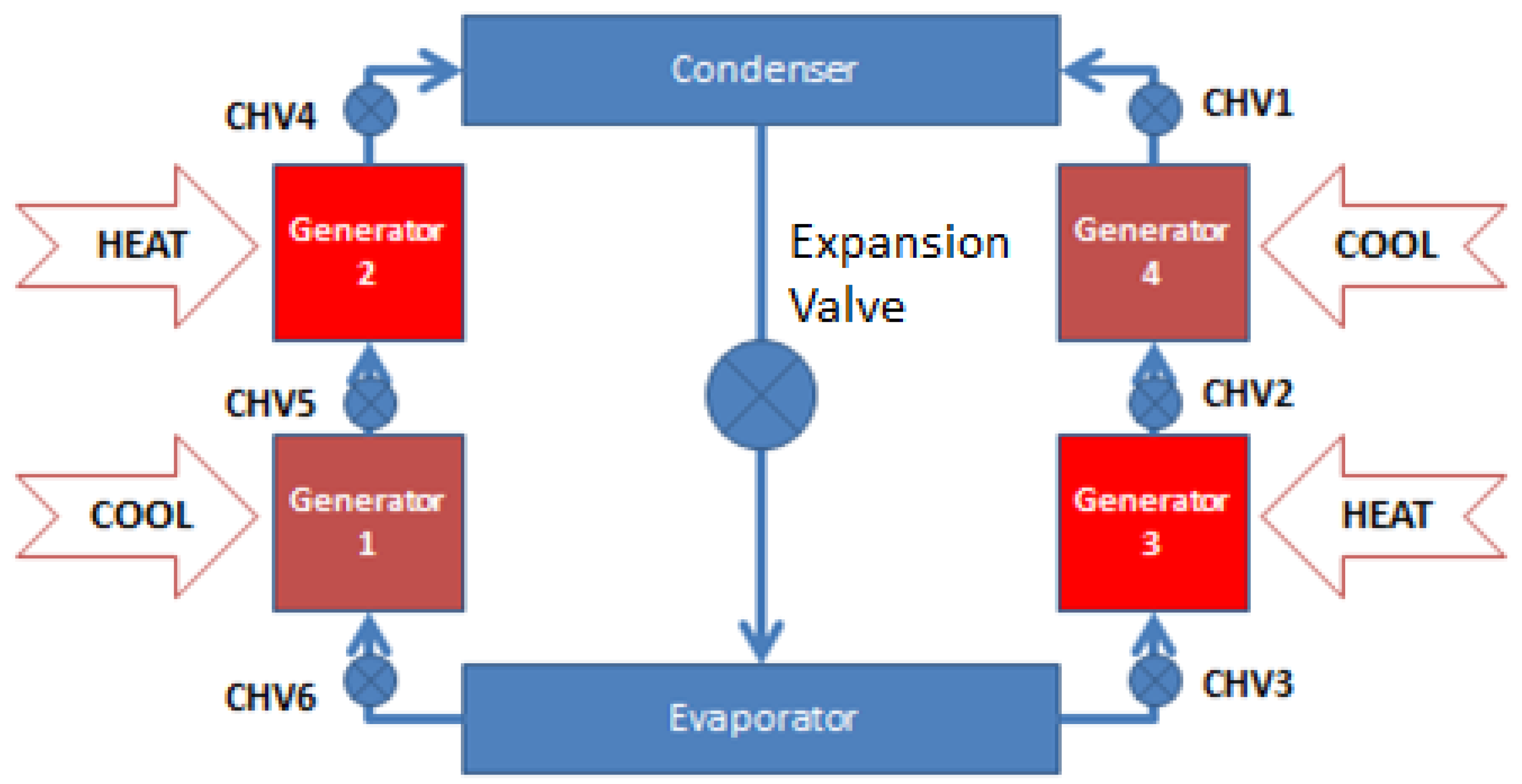
The adsorption chiller under study is comprised of four beds working in two stages, an evaporator, a condenser, valves and pressure and temperature monitoring instruments. In this chiller, the evaporating pressure is halved into two consecutive temperature lifts to exploit the low heat source temperature by introducing two beds for each stage. This configuration makes it possible to run the chiller at hot water temperatures as low as 60 °C and high ambient temperature ranges (up to 50 °C) to produce chilled water as low as 7 °C. The chiller schematic is shown in Figure 1. The chiller was built and operated by Millennium Industries at MU’TAH University since 2012.
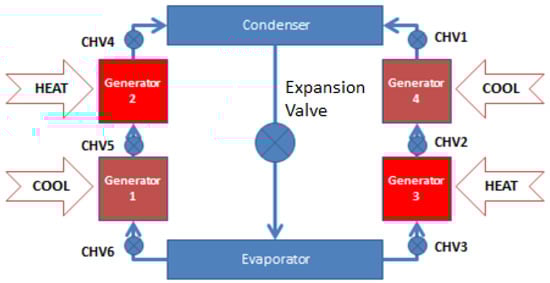
Figure 1.
Schematic for two-stage adsorption chiller.
In the two-stage adsorption chiller, G1 and G3 beds work at low temperature and pressure (close to evaporator pressure), while G2 and G4 beds work at high temperature and pressure (close to condenser pressure). All beds complete four thermodynamic stages. For continuous cooling, each bed of the two-stage adsorption chiller has three time intervals: cooling/heating cycle time, mass and heat recovery time and switching time from heating to cooling and vice versa. During the heating/cooling interval, the adsorption bed interacts with the evaporator, the desorption bed interacts with the condenser, while the other two beds interact with each other.
During the mass and heat recovery interval, the two beds are open to each other (G1 and G3), (G2 and G4) to allow for mass and heat exchange between beds. Hot water and cooling water are not required: condensed methanol is brought back to the evaporator though the expansion valve.
During the switching interval of heating to cooling or vice versa, the adsorption bed is converted to the desorption bed and the desorption bed is converted to the adsorption one by switching the heating and cooling water valves. The beds are isolated from the evaporator and the condenser so there is no mass transfer between beds, evaporator and condenser. The desorption beds are under pre-cooling processes and the adsorption beds are under pre-heating processes.
Modes of Operation for Two Stage Adsorption Chiller
Table 1 shows the operation modes for the two-stage chiller with mass and heat recovery. The two-stage chiller with mass and heat recovery has six modes: modes A, B, C, D, E and F. Table 2 shows valve operation and cooling/hot water circulation.

Table 1.
Operation modes for the two-stage chiller with mass and heat recovery.
Table 2.
Valve operation and cooling/hot water circulation.
2.2. Mathematical Model
2.2.1. Assumptions of the Model
The following assumptions were made to construct the mathematical model.
- Temperature and pressure in the beds, the condenser and the evaporator are uniform.
- Thermodynamic equilibrium exists in the adsorbent bed at any given time.
- The activated carbon granules are treated as a continuous medium.
- Gaseous methanol is treated as an ideal gas.
- Thermal conductivity and specific heats of various components of the system are assumed to be constant in the working temperature range of 293 K to 423 K.
2.2.2. Energy Balance for Two-Stage Chiller with Heat Recovery
The heat exchange for the beds, the evaporator and the condenser, in addition to valves, shown in Figure 1 is used for the mathematical model.
- A.
- During Operation
For G1 and G4: adsorption.
G1 interacts with the evaporator.
G4 interacts with G3. The energy balance equation is:
The left side represents the required sensible heat transfer of activated carbon, the metallic part of the bed and the methanol amount absorbed by activated carbon. The first part of the right side represents the adsorption heat. The second term represents heat flow from evaporator to adsorbent bed. The third term represents the heat transfer by cooling water. The outlet temperature of the cooling water is calculated by Log Mean Temperature Difference (LMTD):
For G2 and G3: desorption, where G2 interacts with condenser. G3 interacts with G4.
The energy balance equation is:
The left side represents the required sensible heat transfer of activated carbon, the metallic part of the bed and the methanol amount absorbed by activated carbon. The first part of the right side represents the desorption heat. The second term represents the heat transfer by heating water. The outlet temperature of the heating water is calculated by LMTD:
For the evaporator:
The left side represents the required sensible heat transfer of the metallic part of the evaporator heat exchanger. is methanol mass inside the evaporator that is changing with time due to adsorption and desorption processes.
The first part of the right side represents latent heat of vaporization for methanol. The second term represents the heat required to cool down incoming condensed methanol at condensation temperature. The last term represents the heat transfer by chilled water.
The outlet temperature of the chilled water is calculated by LMTD:
For the condenser:
The left side represents the required sensible heat transfer of the metallic part of the condenser heat exchanger. The first part of the right side represents latent heat of vaporization for methanol. The second term represents sensible heat transfer from desorber to condenser. The last term represents the heat released by cooling water. The outlet temperature of the condenser water is calculated by LMTD:
- B.
- During switching time
The energy balance equation for the bed switches from adsorption to desorption is:
The energy balance equation for the bed switches from desorption to adsorption is:
For the evaporator:
The outlet temperature of the chilled water is calculated by LMTD:
For the condenser:
The outlet temperature of the condenser water is calculated by Log Mean Temperature Difference (LMTD):
- C.
- Heat Recovery:
G1 is connected to G3: the hot water outlet of G3 is recirculated through G1.
G2 is connected to G4: the hot water outlet of G2 is recirculated through G4.
No external heating or cooling.
For G1 and G2:
For G3 and G4:
For the evaporator:
The outlet temperature of the chilled water is calculated by LMTD:
For the condenser:
The outlet temperature of the condenser water is calculated by LMTD:
- D.
- Isotherm:
Mass Balance
- E.
- Cooling Capacity and COP
3. Results and Discussion
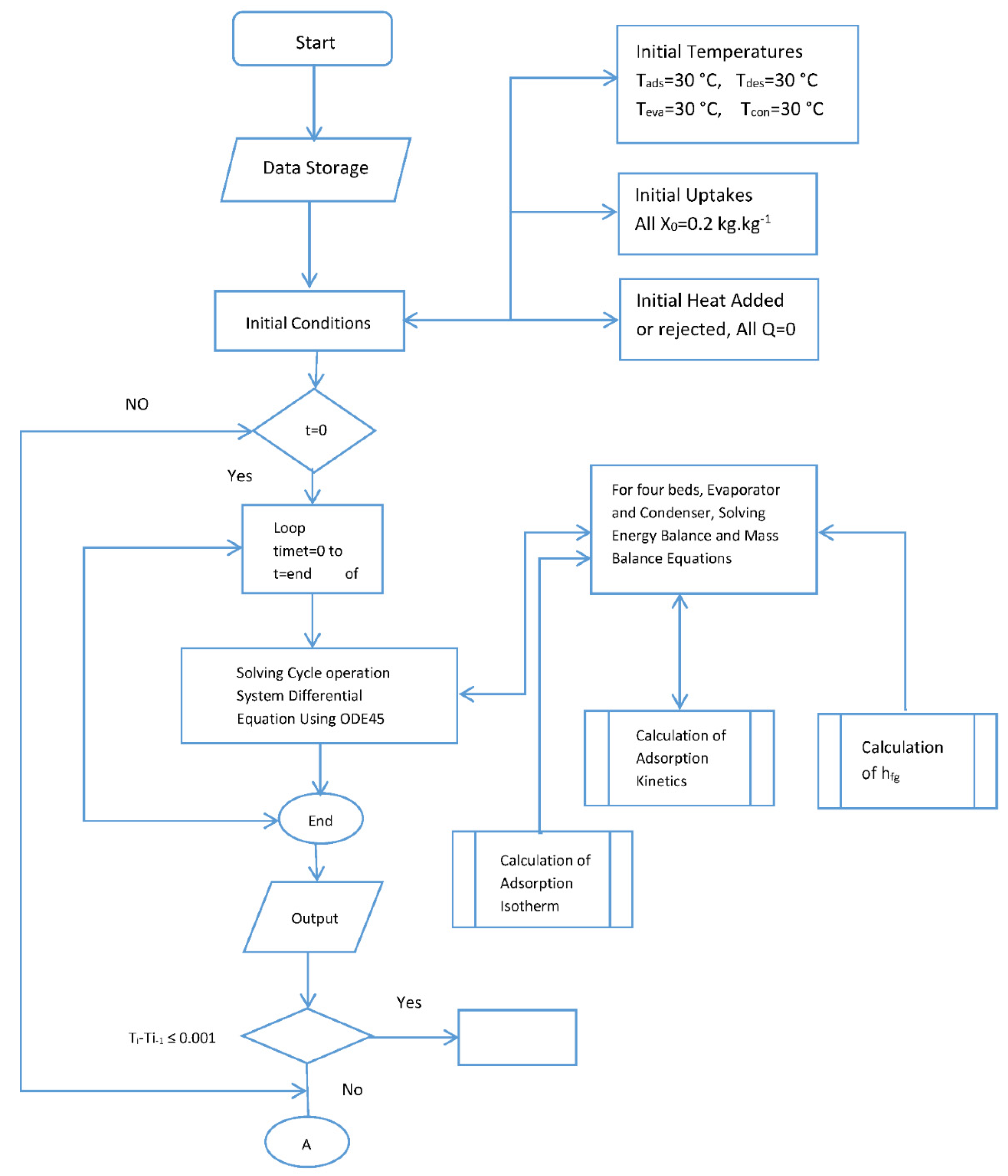
The behavior and performance predictions of the two-stage adsorption chiller are presented here. A series of subroutines were used to calculate the adsorption isotherms and kinetics. The models were used to predict beds temperature, the adsorption isotherm and adsorption kinetics. These coupled equations were solved numerically by MATLAB using ODE 45. Double precision was used, and the tolerance was set to 1 × 10⁻⁶. The computation time was 10 s, the flow chart for the simulation is provided by Appendix A. The flow chart shows that the simulation is started by assigning values for initial temperatures, initial heat added or rejected and initial methanol concentration. The adsorption kinetics and isotherm, enthalpy of formation, feed to energy balance for each of the four beds were calculated and fed to the ODE solver. Temperature end criteria were checked and if satisfied, the, program ended and then COP and cooling capacity were calculated. The same procedure was repeated for the switching time starting from the end of the previous time.
3.1. Model Validation with Experimental Data
The chiller was allowed to operate from transient to cyclic steady state conditions. The key parameters analyzed in the simulation are the temperature profiles for the four beds, the condenser and the evaporator, the coefficient of performance, the effect of heat recovery cycle and the cooling capacity. The values used in the simulation are presented in Appendix B.
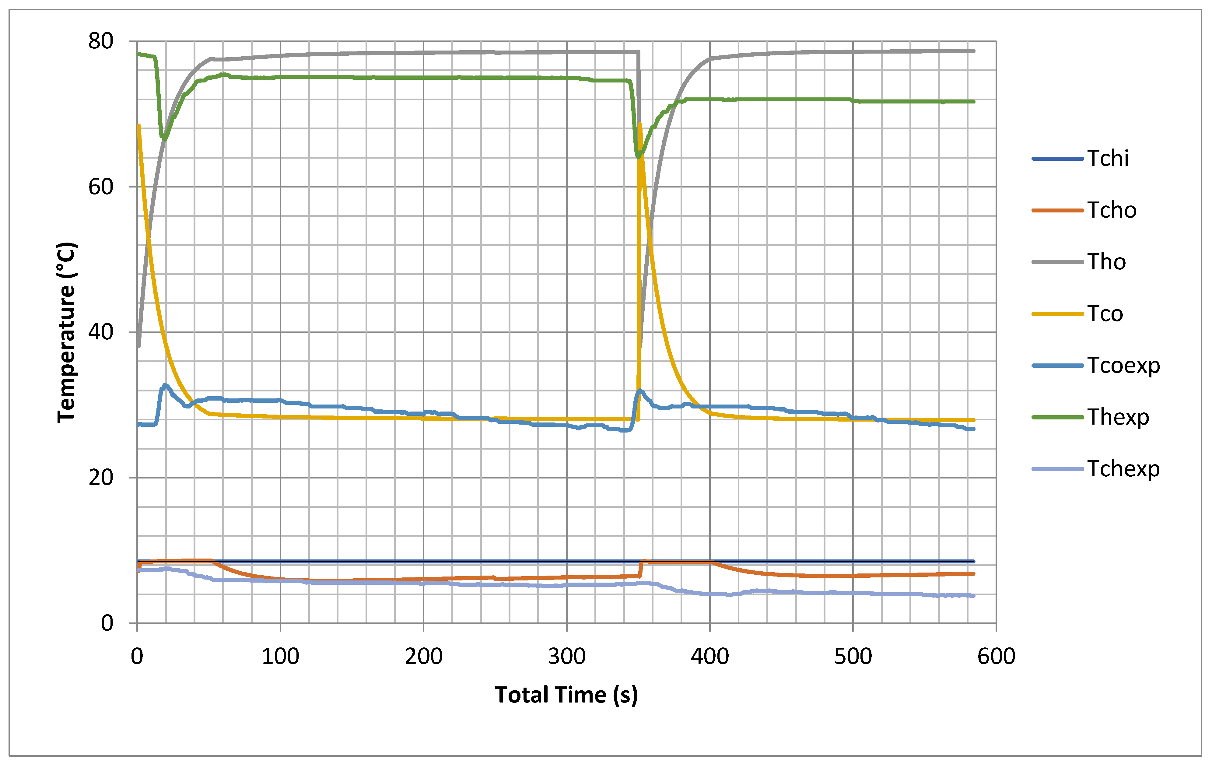
The proposed model predicted temperatures inside the beds, the evaporator and the condenser at one second intervals; thus, the cooling capacity and COP could be evaluated over the cycle and switching time. It is very difficult experimentally to keep constant inlet temperatures for chilled water and cooling and hot water, so the data were measured with varying inlet conditions due to variable solar load use (CSP). In this model, all inlet temperatures were constant, so different outputs were recorded but with same trend as the experimental readings, as shown in Figure 2. The cooling outlet temperature is higher by 5–7 °C than the inlet cooling temperature for both model and experimental results. The chilled water outlet temperature of the model is one degree less than that of the experimental results. This is because the model uses many ideal assumptions as mentioned earlier with regard to the internal heat exchange between heating and cooling water flow during switching from heating to cooling during the experiment.
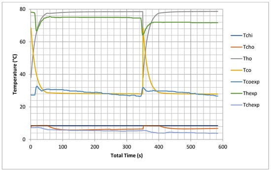
Figure 2.
Experimental validations of outlet temperatures for hot bed, cold bed and chilled water (model results are at chiller nominal operating conditions shown in Appendix C).
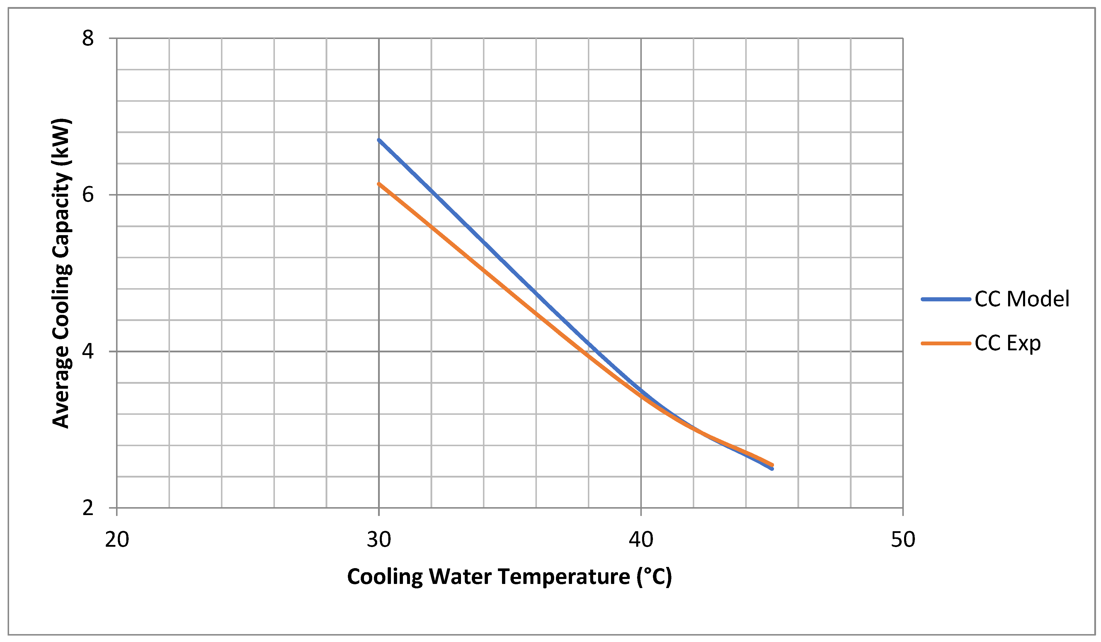
The experimental data for cooling water inlet temperature were time averaged (semi constant) before use in the model. The chiller average cooling capacity coincides very well for both model and experimental results. The average cooling capacity of the model is 110% that of the experimental results at 30 °C and 98% at 45 °C, as shown in Figure 3.
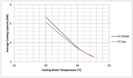
Figure 3.
Comparisons of chiller experimental and model cooling capacity. (Model Results are at Chiller Nominal Operating Conditions shown in Appendix C).
3.2. Optimization of Cycle Times
The adsorption/desorption time was varied while the switching and heat recovery time were kept constant at 30 and 50 s, respectively. All simulated results are at nominal operating conditions as shown in Appendix C.
3.2.1. Cycle Time
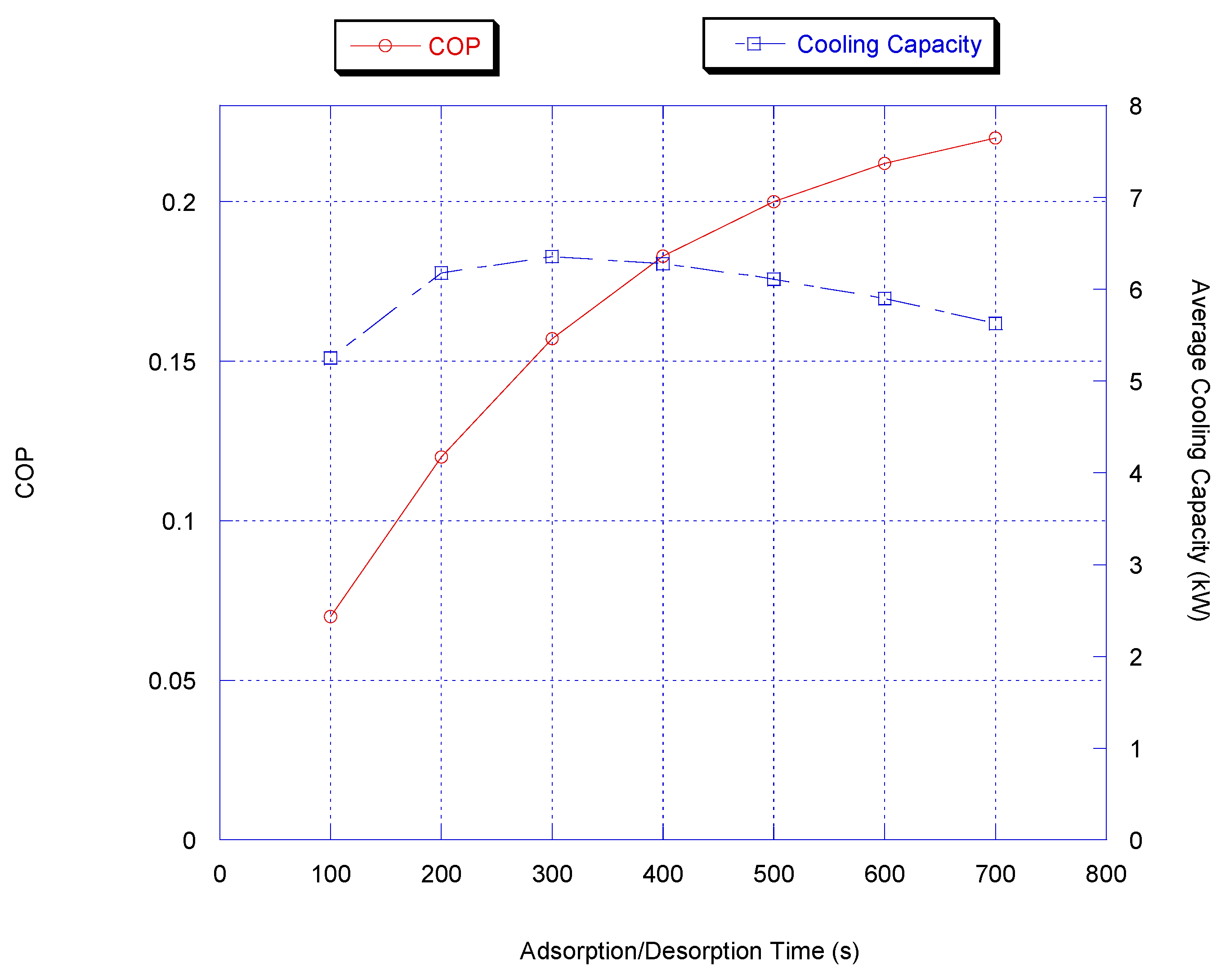
It is clear from Figure 4 that the highest cooling capacity values are attained at the cycle time between 200 and 400 s. When the cycle time is less than 200 s, the cooling capacity decreases abruptly because the adsorption/desorption process does not effectively occur within this short period of time. For cycle times longer than 400 s, the adsorption/desorption process reaches its equilibrium state and so further useful cooling is not foreseen and, as a result, cooling capacity decreases with longer time. For COP, it is observed that COP increases monotonically with cycle time although COP increases with the adsorption/desorption cycle time; the cooling capacity slowly decreases and therefore a 300 to 400 s period was chosen to be the optimum adsorption/desorption cycle time.
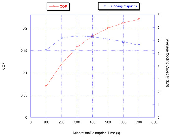
Figure 4.
Effect of cycle time on chiller average cooling capacity.
3.2.2. Switching Time
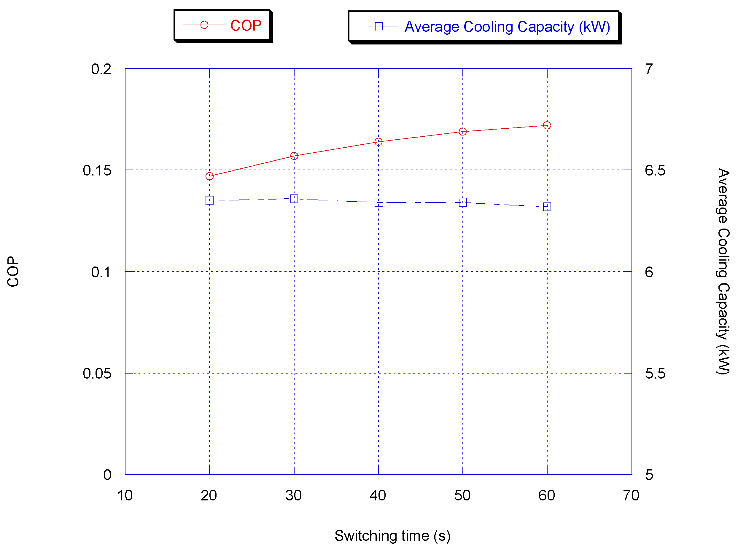
During switching time optimization, the adsorption/desorption and heat recovery times were kept constant at 300 and 50 s, respectively. Figure 5 shows the average cooling capacity and COP. It is very clear that the optimum switching time considering cooling capacity and COP is between 40 and 50 s. The reason is that the beds are fully pre-cooled/pre-heated and further heating/cooling of the beds increases the switching time; thus, the average cooling capacity is reduced since during the switching time, the chiller is not producing a refrigeration effect.
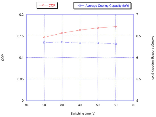
Figure 5.
Effect of switching time on chiller average cooling capacity and COP with heat.
3.2.3. Heat Recovery Time
For heat recovery time optimization, the adsorption/desorption and switching times were kept constant at 300 and 50 s, respectively; the cooling capacity and COP predicted by the model are presented in Figure 6. It is very clear that the optimum heat recovery time considering cooling capacity and COP is between 20 and 30 s while the variation in average capacity is very small.
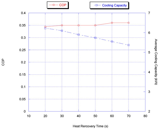
Figure 6.
Effect of heat recovery time on chiller average cooling capacity and COP.
Since the increase in heat recovery time reduced the average cooling capacity and increased the COP, a compromise of 30 s for heat recovery time was chosen.
3.3. Two-Stage Chiller Performance Model Simulation
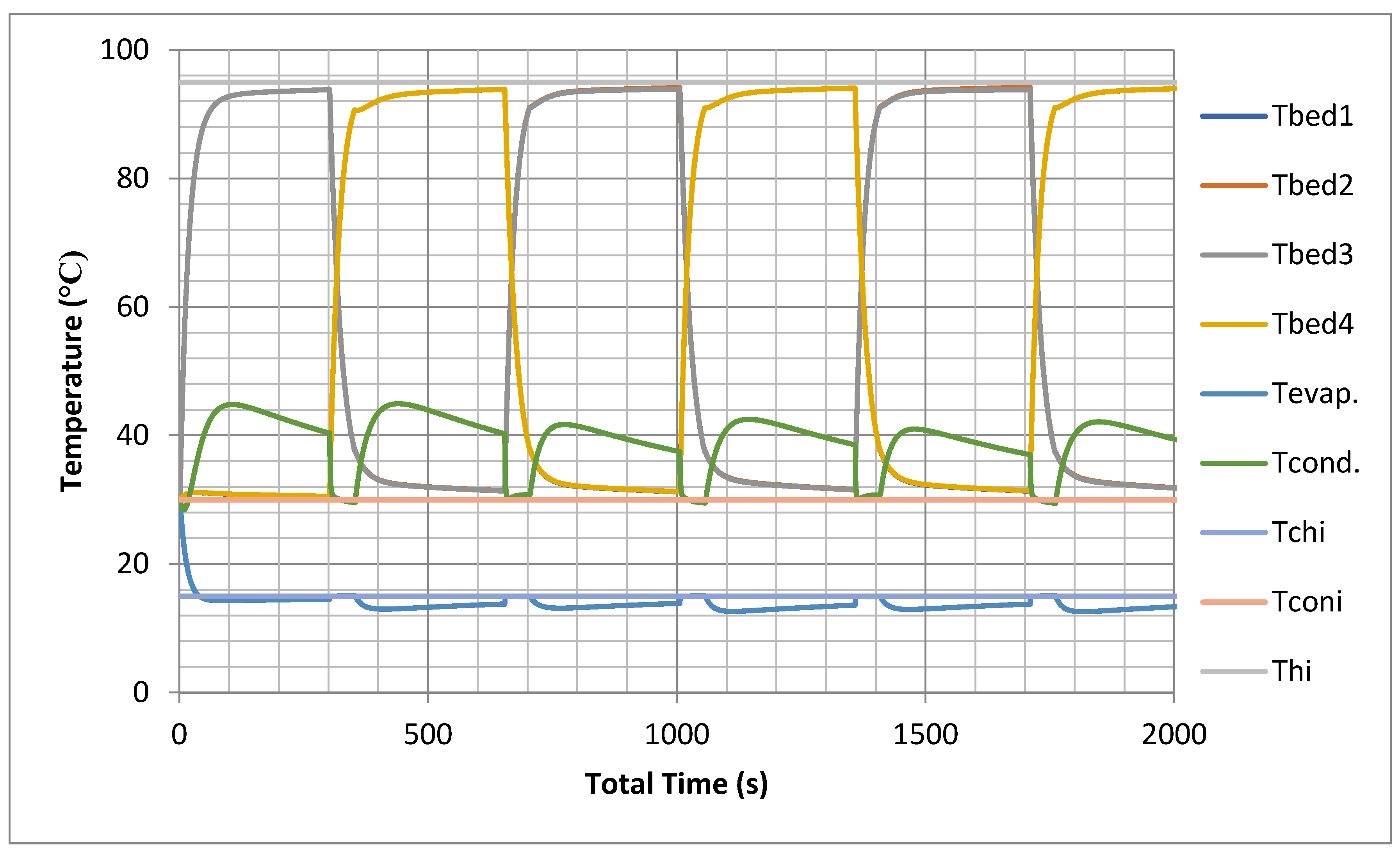
The prediction of temporal histories for the four beds, in addition to the evaporator and the condenser, using models is shown in Figure 7. The temperature profiles are simulated at nominal operating conditions as shown in Appendix C.

Figure 7.
Temporal history of bed, evaporator and condenser temperatures without heat recovery.
The prediction of temporal histories for the four beds, in addition to the evaporator and the condenser, using models is shown in Figure 7 and Figure 8. The temperature profiles are simulated at 95 °C and 30 °C for the heat source and cooling temperatures, respectively.
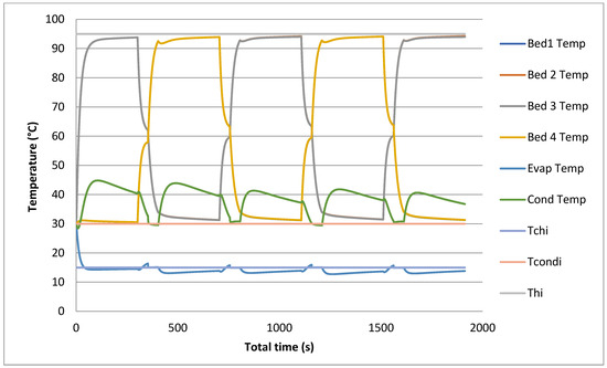
Figure 8.
Temporal history of bed, evaporator and condenser temperatures with heat recovery.
All these temperature profiles are used to calculate the outlet temperature by using LMTD and then to calculate cooling capacity and COP. The heat recovery model includes an adsorption/desorption time, heat recovery time and switching time. The heat recovery cycle is introduced before the switching cycle to reduce the heat required by the desorption bed and to cool down the cooled water required by the desorption bed.
It is very clear that during the heat recovery cycle, the outlet temperature of heated beds and cooled ones reach a temperature level determined by both heating water and cooling water temperatures (50 to 55 °C). The heat recovered is the difference between the heating source temperature and the recovered outlet temperature.
3.3.1. Effect of Operating Conditions
In the adsorption chiller, the operating, heat source and cooling temperatures have a major influence on the cooling capacity and COP.
Effect of Heating Source Temperature
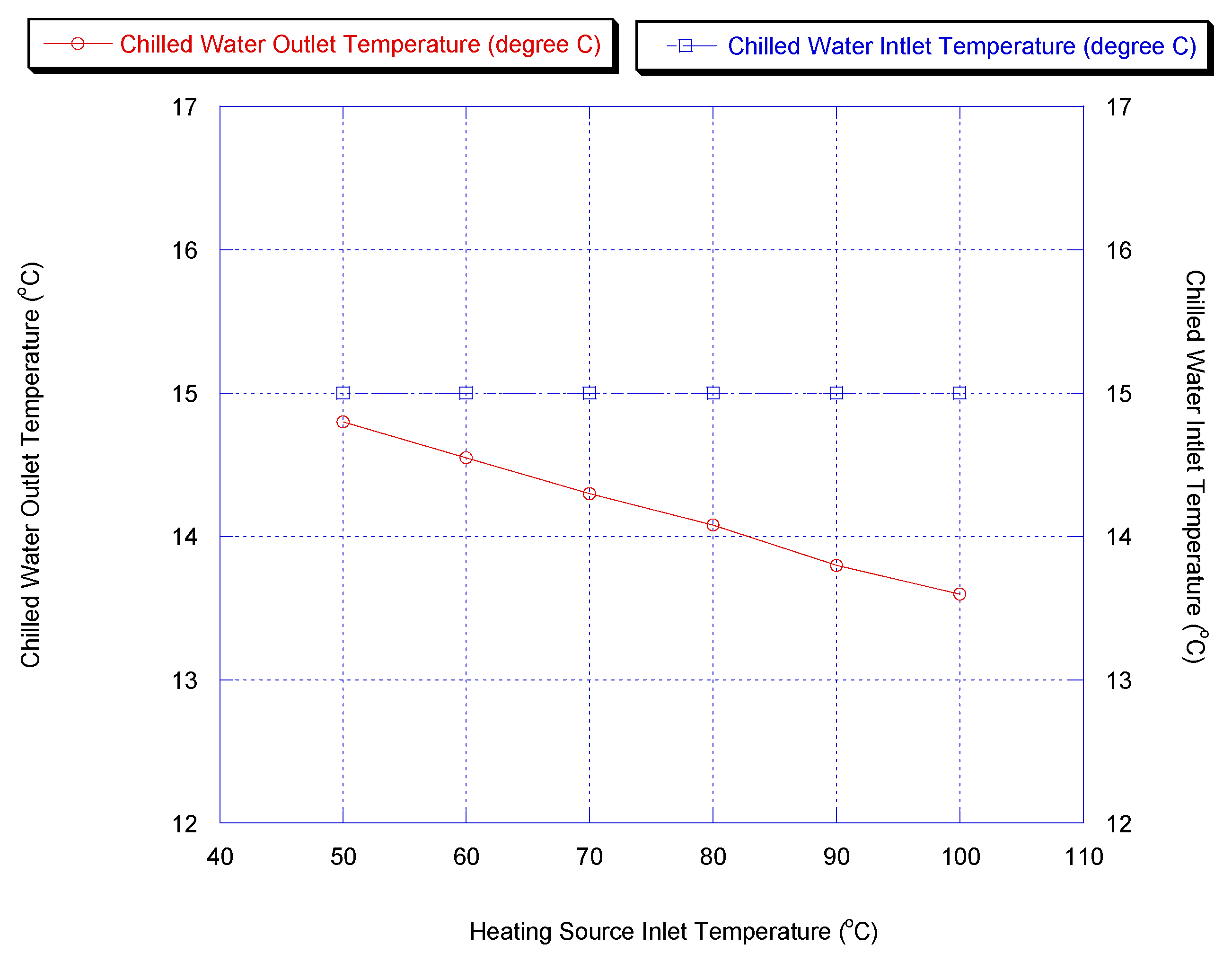
As the driving force, the hot water inlet temperature is one of the key parameters for the adsorption chiller. Figure 9 shows the cooling capacity and COP for the two-stage chiller with heat recovery cycle, if the heating source temperature was varied. Furthermore, chiller water outlet temperature versus heating source temperature is shown in Figure 10. It is shown that a lower chilled water temperature could be produced by increasing the heating source temperature. This is because methanol vapor is desorbed faster at a higher desorption temperature.
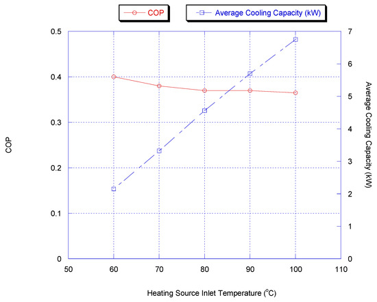
Figure 9.
Effect of heating source temperature on chiller average cooling capacity and COP with heat.
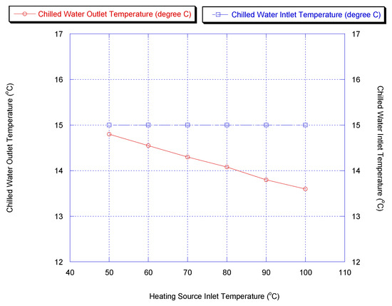
Figure 10.
Effect of heating source temperature on chiller outlet temperature.
The average cooling capacity increases from 1 kW to 7 kW when the heating source temperature increases from 50 °C to 100 °C due to the higher methanol concentration level. The COP increases with increasing the heating source temperature.
The cooling capacity increased sharply and the outlet temperature of chilled water decreased with increasing heating source temperature since the methanol is desorbed faster at a higher desorption temperature, causing more methanol to be adsorbed during the next adsorption process.
Effect of Chilled Water Inlet Temperature
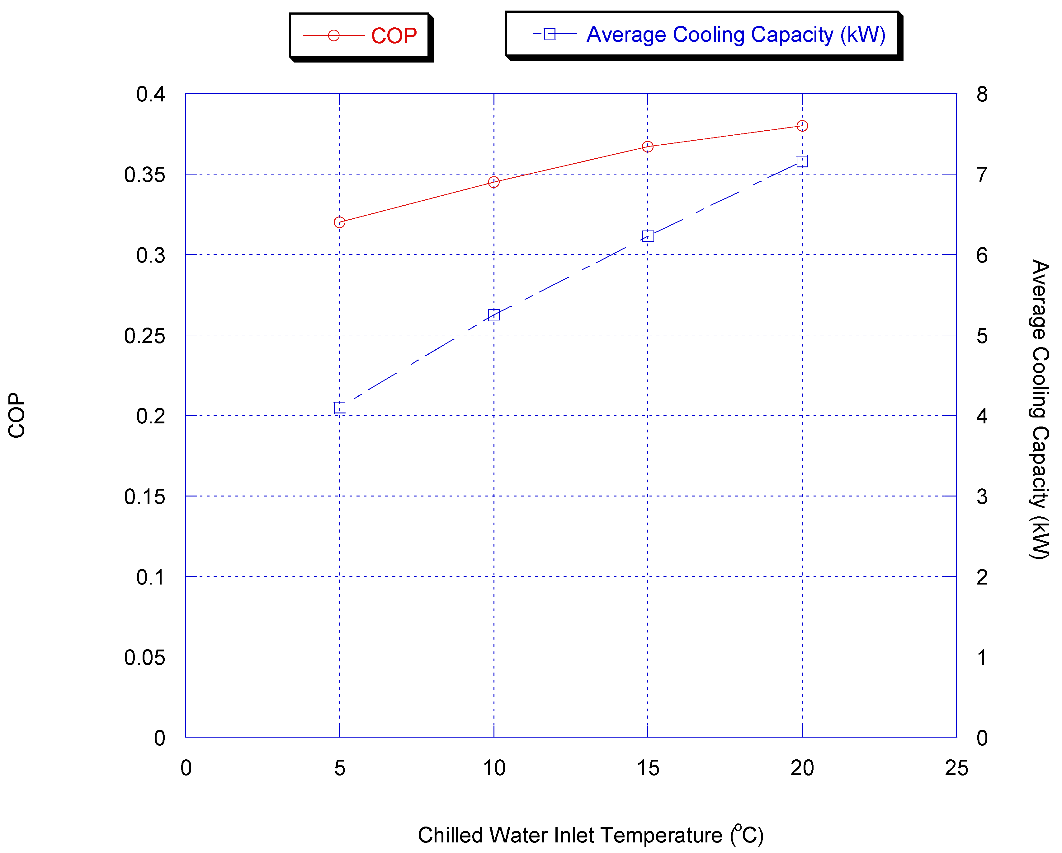
In this part, the influence of changing the evaporating temperature was investigated by varying the inlet temperature of the chilled water. Figure 11 shows the effect of inlet chiller temperature on chiller average cooling capacity and COP with heat recovery.
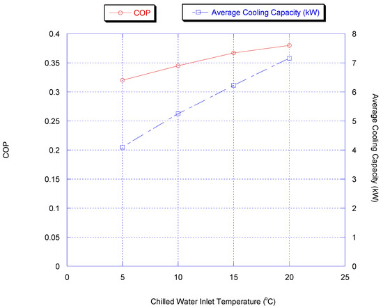
Figure 11.
Effect of inlet chiller temperature on chiller average cooling capacity and COP with heat recovery.
The COP increases with increasing evaporating temperature since, in that case, the higher concentration variation of methanol can be achieved, which increases the heat required for adsorption and desorption and so prolongs cycle time.
Effect of Cooling Water Inlet Temperature
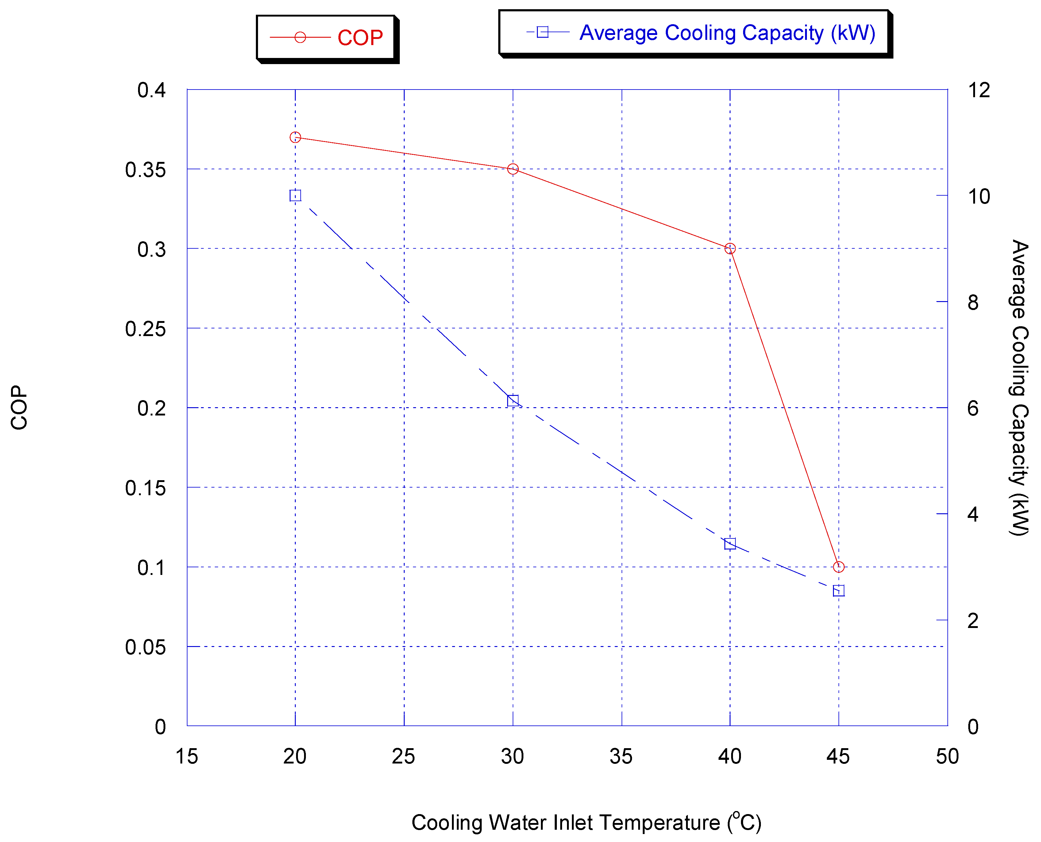
The influence of changing cooling water temperature was investigated by changing the inlet temperature of the cooling water. The cooling water temperature is a very critical actor for both adsorption and condensation processes. Figure 12 shows the effect of inlet cooling water temperature on chiller average cooling capacity and COP with heat recovery.
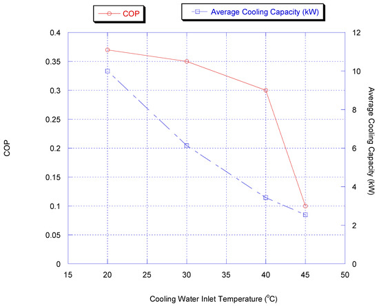
Figure 12.
Effect of inlet cooling water temperature on chiller average cooling and COP capacity with heat recovery.
It is very obvious that cooling capacity and COP increased by lowering the cooling water temperature. This is because more methanol vapor is adsorbed at lower temperature for a given cycle time.
Comparison with Carnot Cycle COP
The COP of the Carnot cycle was used to evaluate model results since it provides the maximum COP that could be achieved at given operating conditions. The chiller allowed for running at optimum parameters for mass flow rates, switching time, cycle time, heat recovery time, optimum heat transfer coefficients for beds and evaporator heat exchangers, in addition to optimized activated carbon mass. The results of the model were compared with Carnot cycle COPs at different chiller nominal operating conditions except hot water inlet temperature. The chiller without heat recovery mode achieved a very low COP when compared with the Carnot cycle COP, while the heat recovery mode results were very close to the Carnot cycle COP, as shown in Table 3.
Table 3.
Carnot cycle COP at different heating source input temperatures.
4. Conclusions
Simulation results were compared with experimental results previously obtained by Millennium Industries. From the simulation results, the following conclusions were drawn:
- The model could predict optimum parameters for cycle time, heat recovery time, switching time, activated carbon mass and mass flow rates for bed, condenser and evaporator heat exchangers.
- The simulation model results agreed well with experimental data in terms of cooling capacity up to 7 kW and Coefficient of Performance (COP) up to 0.4.
- The simulation model showed a transition period of 1000 s to reach a steady state, which is equal to three complete adsorption/desorption cycles.
- The model optimized the adsorption/desorption cycle time (300 to 400 s), switching cycle time (50 s) and heat recovery cycle time (30 s). The optimized times maximized both cooling capacity and COP up to 0.4.
- The COP predicted by this simulation is very close to the Carnot cycle for the heat recovery mode working at the same operating conditions (95%).
- The chiller without heat recovery mode achieved a very low COP when compared with the Carnot cycle COP and the COP for heat recovery mode at the same operating conditions.
- The water outlet temperatures for beds, evaporator and condenser predicted by the simulation agreed, to a reasonable extent, with the experimental data.
- Increasing the cycle time increases the degree to which the capacity of the bed is used. However, increasing the cycle time up to a certain value increases the average system power, and if the cycle time is increased further, the increase in the capacity per cycle is less than that of the increase in cycle time. In other words, as cycle time is increased further, the average power decreases. Then, there exists a certain cycle time for optimal average system power, which is between 300–400 s.
- The heat recovery mode has a COP higher than that of the ordinary mode and has almost the same cooling capacity over a wide range of operating conditions.
- The model predicts different sizes of the chiller for activated carbon/methanol pairs and could be used with minor modifications for other working pairs at the same conditions.
- The two-stage chiller could be driven by using low waste energy with a low COP or a high temperature heat source with a high COP compared with the Carnot cycle COP.
- This study could be used as a basis for series production of a two-stage air cooled adsorption chiller.
- The model will be used for further studies including a desalination function added to the current chiller and integration with other systems such as turbines or any form of hybrid cogeneration.
Author Contributions
Conceptualization, F.M.M. and A.A.A.-M.; methodology, F.M.M.; software, F.M.M.; validation, F.M.M., A.A.B. and A.A.A.-M.; formal analysis, F.M.M.; investigation, H.A.; resources, A.A.; data curation, A.A.; writing—original draft preparation, F.M.M.; writing—review and editing, A.A. and H.A.; visualization, F.M.M.; supervision, A.A.A.-M. and A.A.B.; project administration, F.M.M. All authors have read and agreed to the published version of the manuscript.
Funding
This research received no external funding.
Institutional Review Board Statement
Not applicable.
Informed Consent Statement
Not applicable.
Data Availability Statement
All data are included within manuscript.
Conflicts of Interest
The authors declare no conflict of interest.
Nomenclature
| Symbol | Description | Unit |
| Abed | Bed area | (m2) |
| Aeva | Evaporator area | (m2) |
| Acon | Condenser area | (m2) |
| Cp | Specific heat capacity | (kJ/kg.°C) |
| CC | Cooling Capacity | (kW) |
| COP | Coefficient of Performance | |
| Dso | Surface specific heat | (m2.s−1) |
| Ea | Activation energy | (kJ) |
| hfg | Latent heat of vaporization | (kJ.kg−1) |
| H | Enthalpy | (kJ.kg−1) |
| K | Constant in D-A equation | Non dimensional |
| Meva | Evaporator mass | (kg) |
| Mcon | Condenser mass | (kg) |
| Mac | Mass of activated carbon in each bed | (kg) |
| Meva,m | Mass of methanol in evaporator at t = 0 | (kg) |
| Mcon,m | Mass of methanol in condenser | (kg) |
| N | Constant in D-A equation | Non dimensional |
| P | Pressure | (Bar) |
| Qst | Adsorption heat | (kJ.kg−1) |
| R | Universal gas constant | (kJ/mol. K) |
| T | Temperature | (°C) |
| T | Time | (s) |
| Ubed | Bed overall heat transfer coefficient | (kW/m2.°C) |
| Ueva | Evaporator overall heat transfer coefficient | (kW/m2.°C) |
| Ucon | Condenser overall heat transfer coefficient | (kW/m2.°C) |
| X | Methanol concentration | (kg.kg−1) |
| xo | Maximum methanol concentration | (kg.kg−1) |
| x* | Equilibrium methanol concentration | (kg.kg−1) |
| Subscripts | ||
| ac | activated carbon | |
| ad | adsorption | |
| Al | Aluminum | |
| b | bed | |
| ci | cooling inlet | |
| co | cooling outlet | |
| cw | cold water | |
| chw | chilled water | |
| conw | condenser water | |
| con | condenser | |
| des | desorption | |
| eva | evaporator | |
| fg | vaporization | |
| g | gas | |
| hw | hot water | |
| i | inlet | |
| o | outlet | |
| recw | recalculated water | |
| s | solid | |
| sat | saturation | |
| st | storage |
Appendix A
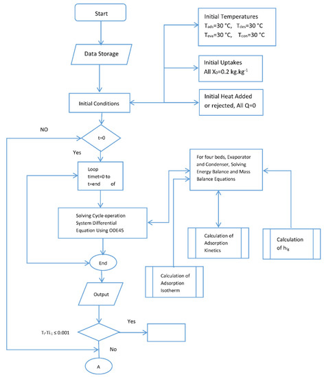
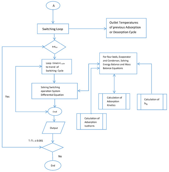
Figure A1.
Flow chart for the simulation.
Figure A1.
Flow chart for the simulation.

Appendix B
Table A1.
Parameters Used in Simulation.
Table A1.
Parameters Used in Simulation.
| Symbol | Value | Unit |
|---|---|---|
| Abed | 4.5 | m2 |
| Aeva | 3 | m2 |
| Acon | 3 | m2 |
| Ubed | 3 | kW/m2.°C |
| Ueva | 2 | kW/m2.°C |
| Ucon | 4 | kW/m2.°C |
| Cpeva | 0.65 | kJ/kg.°C |
| Cpcon | 0.65 | kJ/kg.°C |
| Cpw | 4.18 | kJ/kg.°C |
| Cpac | 1 | kJ/kg.°C |
| Cpm | 2.6 | kJ/kg.°C |
| Meva | 20 | kg |
| Mcon | 30 | kg |
| hfg | 1200 | kJ.kg−1 |
| Mac | 40 | kg |
| Meva,m | 20 at time = 0 | kg |
| Mcon,m | 5 | kg |
| (E/R) Methanol | 978 | K |
| (15 Dso/R) Methanol | 7.35 × 10⁻² | S−1 |
| xo | 0.284 | kg.kg−1 |
| n | 1.39 | Non dimensional |
| K | 10.21 | Non dimensional |
| R1 | 260 | Non dimensional |
| Q | 4.666 | Non dimensional |
| A | 20.84 | Non dimensional |
| B | 4696 | Non dimensional |
Appendix C
Table A2.
Chiller Nominal Operating Conditions.
Table A2.
Chiller Nominal Operating Conditions.
| Symbol | Value | Unit |
|---|---|---|
| Thi | 95 | °C |
| Tci | 30 | °C |
| Tconi | 30 | °C |
| Tchi | 15 | °C |
| Mchw | 2 | kg.s−1 |
| Mcw | 1 | kg.s−1 |
| Mhw | 1.5 | kg.s−1 |
| Mconw | 2 | kg.s−1 |
| Mrecw | 1 | kg.s−1 |
| Adsorption time | 300 | second |
| Desorption time | 300 | second |
| Switching time | 50 | second |
| Heat recovery time | 30 | second |
References
- Modupe, A.O.; Boukhanouf, R. Development Trend of Solar-powered Adsorption Refrigeration Systems: A Review of Technologies, Cycles, Applications, Challenges and Future Research Directions. Development 2019, 6, 10491–10504. [Google Scholar]
- Al-Maaitah, A.A.; Al-Maaitah, A. Two-Stage Low Temperature Air Cooled Adsorption Cooling Unit. U.S. Patent 2011/0113796A1, 19 May 2011. [Google Scholar]
- Sakoda, A.; Suzuki, M. Fundamental study on solar powered adsorption cooling system. J. Chem. Eng. Jpn. 1984, 17, 52–57. [Google Scholar] [CrossRef] [Green Version]
- Makahleh, F.; Badran, A.; Attar, H.; Amer, A.; Al-Almaaitah, A. Modeling and simulation of a two stage adsorption chiller with heat recovery, Part 2. J. Appl. Sci. 2022, 12, 5156. [Google Scholar] [CrossRef]
- Krzywanski, J.; Grabowska, K.; Sosnowski, M.; Żyłka, A.; Sztekler, K.; Kalawa, W.; Wójcik, T.; Nowak, W. Modeling of a re-heat two-stage adsorption chiller by AI approach. MATEC Web Conf. 2018, 240, 05014. [Google Scholar]
- Rajesh, B.; Rajan, A.J. Design and Analysis of a Two-Stage Adsorption Air Chiller. IOP Conf. Ser. Mater. Sci. Eng. 2017, 197, 12030. [Google Scholar]
- Sosnowski, M.; Grabowska, K.; Krzywański, J.; Nowak, W.; Sztekler, K.; Kalawa, W. The effect of heat exchanger geometry on adsorption chiller performance. IOP Conf. Ser. J. Phys. Conf. Ser. 2018, 1101, 012037. [Google Scholar]
- Schwamberger, V.; Desai, A.; Schmidt, F.P. Novel Adsorption Cycle for High-Efficiency Adsorption Heat Pumps and Chillers: Modeling and Simulation Results. Energies 2020, 13, 19. [Google Scholar]
- Jobard, X.; Padey, P.; Guillaume, M.; Duret, A.; Pahud, D. Development and Testing of Novel Applications for Adsorption Heat Pumps and Chillers. Energies 2020, 13, 615. [Google Scholar] [CrossRef] [Green Version]
- Lee, J.-G.; Bae, K.J.; Kwon, O.K. Performance Investigation of a Two-Bed Type Adsorption Chiller with Various Adsorbents. Energies 2020, 13, 2553. [Google Scholar]
- Rouf, R.A.; Jahan, N.; Alam, K.C.A.; Sultan, A.A.; Saha, B.B.; Saha, S.C. Improved cooling capacity of a solar heat driven adsorption chiller. Case Stud. Therm. Eng. 2020, 13, 1–19. [Google Scholar]
- Abd-Elhady, M.M.; Hamed, A.M. Effect of fin design parameters on the performance of a two-bed adsorption chiller. Int. J. Refrig. 2020, 113, 164–173. [Google Scholar] [CrossRef]
- Basdanis, T.; Tsimpoukis, A.; Valougeorgis, D. Performance optimization of a solar adsorption chiller by dynamically adjusting the half-cycle time. Renew. Energy 2021, 164, 362–374. [Google Scholar] [CrossRef]
- Krzywanski, J.; Grabowska, K.; Sosnowski, M.; Zylka, A.; Sztekler, K.; Kalawa, W.; Wojcik, T.; Nowak, W. An adaptive neuro-fuzzy model of a re-heat two-stage adsorption chiller. Therm. Sci. 2019, 23, 1053–1063. [Google Scholar] [CrossRef] [Green Version]
- Miyazaki, T.; Akisawa, A.; Saha, B. The performance analysis of a novel dual evaporator type three-bed adsorption chiller. Int. J. Refrig. 2010, 33, 276–285. [Google Scholar] [CrossRef]
- Alam, K.C.A.; Saha, B.B.; Hamamoto, T.; Akisaw, A.; Kashiwagi, T. Influence of Design and Operating Conditions on The Performance of a Two-Stage Adsorption Chiller. Chem. Eng. Comm. 2006, 91, 981–997. [Google Scholar] [CrossRef]
- Stefański, S.; Mika, L.; Sztekler, K.; Kalawa, W.; Lis, L.; Nowak, W. Adsorption bed configureurations for adsorption cooling application, E3S Web of Conferences 108. Energy Fuels 2019, 2018, 1–10. [Google Scholar]
- Rezk, A.; Al-Dadah, R. Physical and operating conditions effects on silica gel/water adsorption chiller performance. Appl. Energy 2012, 89, 142–149. [Google Scholar] [CrossRef]
- Rahman, A.F.M.M.; Ueda, Y.; Akisawa, A.; Miyazaki, T.; Saha, B.B. Design and Performance of an Innovative Four-Bed, Three-Stage Adsorption Cycle. Energies 2013, 6, 1365–1384. [Google Scholar] [CrossRef] [Green Version]
- Saha, B.B.; Boelman, E.C.; Kashiwagi, T. Computational analysis of an advanced adsorption-refrigeration cycle. Energy 1995, 20, 983–994. [Google Scholar] [CrossRef]
- Saha, B.; Koyama, S.; Lee, J.; Kuwahara, K.; Alam, K.; Hamamoto, Y.; Akisawa, A.; Kashiwagi, T. Performance evaluation of a low-temperature waste heat driven multi-bed adsorption chiller. Int. J. Multiph. Flow 2003, 29, 1249–1263. [Google Scholar] [CrossRef]
- Saha, B.B.; Koyama, K.; Akisawa, A.; Kashiwagi, T.; Ng, K.C.; Chua, H.T. Waste Heat Driven Multi-Stage, Multi-Bed Regeneration Adsorption System. Int. J. Refrig. 2003, 26, 749–757. [Google Scholar] [CrossRef]
- Schicktanz, M.; Hügenell, P.; Henninger, S. Evaluation of methanol/activated carbons for thermally driven chillers, part II: The energy balance model. Int. J. Refrig. 2012, 35, 554–561. [Google Scholar]
- Wang, L.; Wu, J.; Wang, R.; Xu, Y.; Wang, S. Experimental study of a solidified activated carbon-methanol adsorption ice maker. Appl. Therm. Eng. 2003, 23, 1453–1462. [Google Scholar] [CrossRef]
- Wang, J.; Wang, L.W.; Luo, W.L.; Wang, R.Z. Experimental Study of a Two-Stage Adsorption Freezing Machine Driven by Low Temperature Heat Source. Int. J. Refrig. 2013, 36, 1029–1031. [Google Scholar] [CrossRef]
- Wirajatia1, I.G.A.B.; Widiantaraa, I.B.G.; Arditaa, I.N. Simulation and experimental verification on re-heat two-stage adsorption refrigeration cycle. J. Appl. Mech. Eng. Green Technol. 2019, 1, 25–30. [Google Scholar]
- Chua, H.T.; Ng, K.C.; Malek, A.; Kashiwagi, T.; Akisaw, A.; Saha, B.B. Modeling the Performance of Two-Bed, Silica gel-water Adsorption Chiller. Int. J. Refrig. 1999, 22, 194–204. [Google Scholar] [CrossRef]
- Miyazaki, T.; Akisawa, A.; Saha, B.B.; El-Sharkawy, I.I.; Chakraborty, A. Anew Cycle Time Allocation for Enhancing the Performance of Two-Bed Adsorption Chiller. Int. J. Refrig. 2009, 32, 846–853. [Google Scholar] [CrossRef]
- Hassan, H.; Mohamad, A.; Al-Ansary, H. Development of a continuously operating solar-driven adsorption cooling system: Thermodynamic analysis and parametric study. Appl. Therm. Eng. 2012, 48, 332–341. [Google Scholar]
- Alam, K.A.; Saha, B.B.; Akisawa, A.; Kashiwagi, T. A Novel Parametric Analysis of a Conventional Silica-Gel Water Adsorption Chiller. Trans. Jpn. Soc. Refrig. Air Cond. Eng. 2011, 17, 323–332. [Google Scholar]
- Mohammed, R.H.; Mesalhy, O.; Elsayed, M.L.; Chow, L.C. Novel compact bed design for adsorption cooling systems: Parametric numerical study. Int. J. Refrig. 2012, 80, 238–251. [Google Scholar]
- Papoutsis, E.; Koronaki, I.; Papaefthimiou, V. Numerical simulation and parametric study of different types of solar cooling systems under Mediterranean climatic conditions. Energy Build. 2017, 138, 601–611. [Google Scholar] [CrossRef]
- Papoutsis, E.G.; Koronaki, I.P.; Papaefthimiou, V.D. Parametric Study of a Single-Stage Two-Bed Adsorption Chiller. J. Energy Eng. 2017, 4, 04016068. [Google Scholar] [CrossRef]
- Agrouaz, Y.; Bouhal, T.; Allouhi, A.; Kousksou, T.; Jamil, A.; Zeraouli, Y. Energy and parametric analysis of solar absorption cooling systems in various Moroccan climates. Case Stud. Therm. Eng. 2017, 9, 28–39. [Google Scholar] [CrossRef]
- Al-Rbaiha, R.; Sakhrieh, A.; Al-Asfar, J.; Alahmer, A.; Ayadi, O.; Al-Salaymeh, A.; Al_hamamre, Z.; Al-bawwab, A.; Hamdan, M. Performance Assessment and Theoretical Simulation of Adsorption refrigeration System Driven by Flat Plate Solar Collector. Jordan J. Mech. Ind. Eng. 2017, 11, 1–11. [Google Scholar]
- Sztekler, K.; Kalawa, W.; Nowak, W.; Mika, L.; Gradziel, S.; Krzywanski, J.; Radomska, E. Experimental Study of Three-Bed Adsorption Chiller with Desalination Function. Energies 2020, 13, 5827. [Google Scholar] [CrossRef]
- Sztekler, K.; Siwek, T.; Kalawa, W.; Lis, L.; Mika, L.; Radomska, E.; Nowak, W. CFD Analysis of Elements of an Adsorption Chiller with Desalination Function. Energies 2021, 14, 7804. [Google Scholar] [CrossRef]
- Sztekler, K.; Kalawa, W.; Mika, L.; Krzywanski, J.; Grabowska, K.; Sosnowski, M.; Nowak, W.; Siwek, T.; Bieniek, A. Modeling of a Combined Cycle Gas Turbine Integrated with an Adsorption Chiller. Energies 2020, 13, 515. [Google Scholar] [CrossRef] [Green Version]


Publisher’s Note: MDPI stays neutral with regard to jurisdictional claims in published maps and institutional affiliations. |
© 2022 by the authors. Licensee MDPI, Basel, Switzerland. This article is an open access article distributed under the terms and conditions of the Creative Commons Attribution (CC BY) license (https://creativecommons.org/licenses/by/4.0/).