Multi-Sensor Fusion for Lateral Vehicle Localization in Tunnels

Abstract

The satellite navigation signal in the tunnel is weak, and it is difficult to achieve accurate lateral positioning in complex conditions such as low-speed congestion by relying solely on inertial navigation or line image recognition, which is one of the problems of automatic driving at present. In this paper, a lane-level location method based on multi-sensor fusion is proposed. Using the machine vision method, detecting lane lines with the monocular camera, and fitting the lane lines to determine the driving status of the vehicle based on the lane line information. The top view of the lane line is taken by the binocular camera, and the distance of the vehicle from the lane line and the width of the lane are calculated from the pictures taken by the binocular camera. Obtaining the heading angle information of the vehicle using the gyroscope in inertial navigation and the distance information of the vehicle using the odometer. When a car changes lanes or overtakes, the new lane the vehicle is in is calculated by calculating the difference in heading angle and combining it with the lane width and odometer information so as to complete the lateral positioning of the vehicle. The simulation results show that the algorithm has high lateral positioning accuracy. The positioning accuracy is less affected by the drift of inertial elements, and the error will not accumulate.

1. Introduction

Smart cars and autonomous driving technology have made very significant advances in the last decade, and vehicle location technology has been a key technology in smart driving. Traditional vehicle positioning techniques [1,2,3,4] include the use of GPS, inertial navigation, image recognition, radar, etc. However, in some complex scenarios, such as in densely built-up areas or long tunnels, GPS can lose lock [5], and lane markings can be obscured on congested roads at low speeds. These conditions can result in existing positioning calculation methods, such as GPS, inertial navigation, vision, and LIDAR not being able to accurately locate the vehicle. The use of a single positioning system or single sensor positioning technology for vehicles is no longer sufficient for the complex traffic conditions of today; therefore, more and more researchers are trying to use multi-sensor fusion localization methods for precise positioning of vehicles [6,7,8,9]. Compared with a single positioning system. The multi-sensor fusion positioning method not only has higher accuracy but also has better robustness and anti-interference.

Qian et al., proposed interactive multi-model filtering (IMM-UKF) method to jointly estimate position information [10], fusing INS with GPS. Compared with the traditional Kalman filter, this algorithm has higher accuracy and convergence speed. Although this algorithm can provide higher accuracy of vehicle pose in a complex urban environment, such a method based solely on satellite signal enhancement and optimization cannot be used in a long tunnel and other GPS signals completely blind area. Zhu proposed a vehicle positioning system that relies only on heading projection and inertial navigation for vehicles that have been out of GPS signal lock for a long time [11]. The experimental results show that the system can effectively reduce the error to achieve effective positioning when the GPS is out of lock for a long time, but it only reduces the error for the longitudinal direction of the vehicle, the lateral positioning error of the vehicle is still large. Yang et al., proposed a high-precision integrated navigation method for land vehicles using SINS, odometer, and Doppler radar [12]. The experimental results of the method show that the positioning accuracy of the vehicle in the absence of a GPS signal of the vehicle compared to only the inertial guidance system has significantly improved. Its horizontal position error although not more than 0.03% of the distance the vehicle travels, but due to the accumulation of its error, the positioning accuracy of the vehicle in the long tunnel will not meet the lateral positioning of the vehicle after traveling a certain distance. A loosely coupled algorithm for relative localization of the visual odometer was proposed by Serov et al. [13], to update the unscented Kalman filter using the relative pose between two frames of the camera. Although it has a lower error than other visual odometer methods, the algorithm only addresses the longitudinal positioning of the vehicle and does not specifically investigate the lateral positioning of the vehicle. Wang et al., used perspective transformation of images captured by a monocular camera for in-lane localization of vehicles [14]. Its positioning has high accuracy but only takes into account the distance of the vehicle from the left and right lane lines when the vehicle is traveling in a certain lane and can be considered a static positioning, which will not be applicable to the dynamic positioning of the vehicle when a lane change occurs. Xin et al., proposed the method of integrating dead reckoning with inertial navigation to solve the problem of vehicle positioning when a GPS signal is lost [15]. Although the positioning accuracy is improved compared with the use of a single inertial navigation system, there is not much research on the lateral positioning of vehicles. Li et al., proposed a close coupling method of inertial navigation and radar to carry out real-time positioning for vehicles [16]. The positioning accuracy can reach centimeter-level, but ordinary radar will weaken or even lose signals in long subsea tunnels. Therefore, this method may not be applicable to such scenarios. Zhang uses image sequences and wheel-inertial ego-motion results to build a local environment map and matches it with the electronic map to locate the vehicle [17]. Liang et al., proposed a multi-sensor fusion slam method for vehicle location [18]. Chen proposed a vehicle autonomous positioning method based on terrain relative navigation [19]. This method matches the terrain data collected by the vehicle during driving with the pre-established topographic map, so as to estimate the position of the vehicle on the topographic map and realize the position of the vehicle on the structured road. References [17,18,19] all proposed the use of electronic maps to accurately locate vehicles. Although this method has high accuracy (including high-precision lateral positioning), however, the establishment of electronic maps or topographic maps requires some real vehicle experiments to obtain topographic data first, which is a huge work and requires a lot of time, and once there is construction in a certain section, the previously established map data may not match with the actual situation.

In this paper, a vehicle lateral positioning algorithm based on heading angle calculated by inertial navigation is proposed to provide high accuracy for vehicle lateral positioning when the GPS signal is locked for a long time. Strapdown inertial navigation uses the quaternion method to update attitude and provide heading angle information. The lane change can be determined by the difference in heading angle in adjacent time. The monocular camera is used to identify and fit the lane lines and calculate the slope and x-axis intersection of the fitted lane lines in the image to assist in determining whether the lane change occurs. A lane change can be identified only when the monocular camera and the heading angle difference simultaneously judge the lane change. The odometer provides information on the distance the vehicle passes in the process of lane change. The lateral displacement of the vehicle can be calculated by combining the difference between the heading angle at the end of a lane change and the beginning of a lane change with odometer data, which has high accuracy. A binocular camera is used to measure the distance between the vehicle and the lane line and the lane width to provide the initial input for the algorithm.

The system proposed in this paper has the following improvements: (1) Most of the traditional inertial navigation and positioning technologies are aimed at the longitudinal positioning of vehicles, and because of the cumulative nature of inertial navigation errors, the positioning error of vehicles will increase with the accumulation of time. The system proposed in this paper is only for the vehicle lane change and overtaking process. The vehicle lane change and overtaking process time is very short, and inertial navigation can provide high accuracy in a short time. The lateral displacement of the vehicle can be calculated by calculating the heading angle of the vehicle through inertial navigation, calculating the difference in heading angle of the vehicle after changing lanes or overtaking, and then combining it with the odometer to calculate the distance information of the vehicle during the driving process. The algorithm has good accuracy and fast computation speed. (2) While many researchers use monocular cameras to calculate the lateral distance of vehicles, this paper proposes to measure the distance of vehicles from the lane line using binocular cameras, the main implementation of which is to mount the binocular camera under the rearview mirror of the vehicle to take a top view of the lane line. In this paper, we propose to use the lane line contour point extraction method to measure the distance of the vehicle from the lane line dynamically and in real-time. Compared with monocular camera ranging, a binocular camera can provide more accurate input to the system.

2. Methods

Figure 1 shows a vehicle lateral positioning system proposed in this paper. The hardware mainly includes the following three subsystems: binocular, monocular, and inertial navigation. Strapdown inertial navigation is the computing core, and monocular and binocular cameras are auxiliary. First of all, before the car enters the tunnel, we set the car to enter the tunnel from the middle lane, so that we can infer the new lane for each lane change in the future. Two binocular cameras were installed below the left and right rearview mirrors of the car to calculate lane width. When the car runs into the tunnel, the binocular camera measures the transverse distance between the optical center and the marking line, and then adds the distance with the optical center of the left and right cameras to obtain the width of the lane line. The monocular camera is installed in the central position of the front of the car. Based on the recognition of lane lines, it can distinguish whether lane change occurs and determine the direction of lane change. When the difference in heading angle at adjacent times is greater than a threshold, the lateral displacement of the vehicle is calculated from the difference in heading angle and the distance information provided by the odometer. At this time, only when the monocular camera also recognizes the lane change of the vehicle, the lateral displacement of the vehicle becomes effective; otherwise, it is determined that the vehicle has not changed lanes. Combined with the lane width calculated by binocular camera, the new lane where the vehicle is located can be obtained to complete the location of the vehicle.

2.1. Attitude Update Algorithm for Strapdown Inertial Navigation

The coordinate systems commonly used in strapdown inertial navigation system include the following: inertial coordinate system (i frame), earth coordinate system (e frame), geographic coordinate system (g frame), navigation coordinate system (n frame), and carrier coordinate system (b frame), etc. In this paper, the East-North-Up (ENU) geographical coordinate system is chosen as the navigation coordinate system, and the right front up is the carrier coordinate system. That is, the origin is the center of gravity of the carrier, the $x_b$ axis is to the right along the horizontal axis of the carrier, the $y_b$ axis is to the front along the vertical axis of the carrier, and the $z_b$ axis is to the top along the vertical axis of the carrier.

Most of the algorithms for inertial navigation fusing multiple sensors are aimed at longitudinal positioning of the vehicle and these algorithms are well established [20,21,22,23]. The focus of this paper is on the lateral positioning of the vehicle. The vehicle lateral positioning algorithm proposed in this paper is based on the difference of heading angles in adjacent time, so a high accuracy heading angle solution is necessary. In this paper, quaternion method [24] is used to update the attitude of strapdown inertial navigation system.

We all know that in a two-dimensional plane coordinate system, the rotation information of an object can be described by the formula $u=cos\theta + \mathit{i} sin\theta$, however, this formula does not apply when it is necessary to represent the rotation information of a three-dimensional space. So when we need to represent the rotation information of a three-dimensional space, we need to use the formula $Q=cos\theta +(\mathit{i}+\mathit{j}+\mathit{k}) sin\theta$ (where i, j, k are the unit vectors of x, y, z axis respectively). We write $Q=cos\theta +(\mathit{i}+\mathit{j}+\mathit{k}) sin\theta$ as $Q=q_0+q_1\mathit{i}+q_2\mathit{j}+q_3\mathit{k}$ to obtain our common quaternion form. Thus, we obtain the following definition of quaternion:

$$Q(q_0,q_1,q_2,q_3)=q_0+q_{1}i+q_{2}j+q_{3}k$$

(1)

In the above equation, $q_0,q_1,q_2,q_3$ are real numbers and i, j, k are both mutually orthogonal unit vectors and imaginary units $\sqrt{-1}$.

The relation between quaternion and attitude matrix is as follows:

$$C_b^R=\left[\begin{array}{ccc}1-2(q_2^2+q_3^2)& 2(q_1{q}_2-q_0{q}_3)& 2(q_1{q}_3+q_0{q}_2)\\ 2(q_1{q}_2+q_0{q}_3)& 1-2(q_1^2+q_3^2)& 2(q_2{q}_3-q_0{q}_1)\\ 2(q_1{q}_3-q_0{q}_2)& 2(q_2{q}_3+q_0{q}_1)& 1-2(q_1^2+q_2^2)\end{array}\right]$$

(2)

Since the quaternion describing the rotation of a rigid body is a normalized quaternion, the normalized quaternion has the following characteristics:

$$\Vert Q\Vert =q_0^2+q_1^2+q_2^2+q_3^2=1$$

(3)

Therefore, the relationship between quaternion and attitude matrix can be further transformed into the following:

$$C_b^R=\left[\begin{array}{ccc}{q}_0^2+q_1^2-q_2^2-q_3^2& 2(q_1{q}_2-q_0{q}_3)& 2(q_1{q}_3+q_0{q}_2)\\ 2(q_1{q}_2+q_0{q}_3)& q_0^2-q_1^2+q_2^2-q_3^2& 2(q_2{q}_3-q_0{q}_1)\\ 2(q_1{q}_3-q_0{q}_2)& 2(q_2{q}_3+q_0{q}_1)& q_0^2-q_1^2-q_2^2+q_3^2\end{array}\right]$$

(4)

Quaternion differential equation of attitude update as follows:

$${\dot{q}}_b^n=\frac{1}{2}{q}_b^n{\omega }_{nb q}^b$$

(5)

In the following formula:

$$\begin{array}{c}{\omega }_{nb}^b={\omega }_{ib}^b-{\omega }_{in}^b={\omega }_{ib}^b-C_n^b{\omega }_{in}^n={\omega }_{ib}^b-{(C_b^n)}^T{\omega }_{in}^n\\ {\omega }_{in}^n={\omega }_{ie}^n+{\omega }_{en}^n\\ {\omega }_{ie}^n={\left[\begin{array}{ccc}0& {\omega }_{ie}\cos L& {\omega }_{ie}\sin L\end{array}\right]}^T\\ {\omega }_{en}^n={\left[\begin{array}{ccc}-\frac{v_N^n}{R_M+h}& \frac{v_E^n}{R_N+h}& \frac{v_E^n}{R_N+h}\tan L\end{array}\right]}^T\end{array}$$

We will explain some parameters in the above formula. $q_b^n$ is the quaternion describing the attitude of the carrier. ${\omega }_{ib}^b$ is the angular velocity of the carrier measured by gyroscope. h is the altitude. $v^n={\left[\begin{array}{ccc}{v}_E^n& v_N^n& v_U^n\end{array}\right]}^T$ is the strapdown inertial navigation velocity. ${\left(V\right)}_q$ is the vector $V$ expressed as a quaternion, as shown in the following formula: ${({\left[\begin{array}{ccc}x& y& z\end{array}\right]}^T)}_q={\left[\begin{array}{cccc}0& x& y& z\end{array}\right]}^T$. $L$ is the latitude value of the vehicle position. $R_M$ and $R_N$ are curvature radius of the earth’s meridian circle and the curvature radius of the unitary circle at the location of the carrier, respectively, and their formula is approximately as follows:

$$R_M\approx R_e(1-2f+3f{\sin }^{2}L)$$

(6)

$$R_N\approx R_e(1+f{\sin }^{2}L)$$

(7)

$R_e$ is the major half-axis of the earth reference ellipsoid, f is the flattening of the reference ellipsoid,

$$R_e=6378137(m),f=\frac{1}{298.257}$$

The attitude update quaternion differential equation is transformed into the following digital recursive form:

$$q_{b_n(m)}^n=q_{b_n(m-1)}^n{q}_{b_n(m)}^{b_n(m-1)}$$

(8)

In the following formula:

$q_{b_n\left(m\right)}^n$ is the attitude quaternion at $t_m$ time, shorthand for $q_{b\left(m\right)}^n$;

$q_{b_n(m-1)}^n$ is the attitude quaternion at $t_{m-1}$ time, shorthand for $q_{b(m-1)}^n$;

$q_{b_n\left(m\right)}^{b_n(m-1)}$ is based on n frame of reference when b frame is from $t_{m-1}$ moment to $t_m$ moment transformation of quaternions, it is going to use ${\mathsf{\omega }}_{nb}^b\left(t\right)$.

Let ${\eta }_m$ be the equivalent rotation vector of b frame relative to n frame from $t_{m-1}$ time to $t_m$ time,

$${\eta }_m={\displaystyle {\int }_{m-1}^m{\omega }_{nb}^b(t)dt}$$

(9)

$${\eta }_m={\displaystyle {\int }_{m-1}^m{\omega }_{ib}^b(t)-{(C_b^n(t))}^T{\omega }_{in}^n(t)dt}$$

(10)

Because ${\omega }_{in}^n\left(t\right)$ changes very slowly compared with ${\omega }_{ib}^n\left(t\right)$, if we consider ${\left(C_b^n\left(t\right)\right)}^T$ and ${\omega }_{in}^n\left(t\right)$ basically unchanged at $t_{m-1}\le t \le t_m$, and let them be the values of $t_{m-1}$, then we have

$${\eta }_m\approx {\displaystyle {\int }_{m-1}^m{\omega }_{ib}^b(t)dt-{(C_{b(m-1)}^n)}^T{\omega }_{in(m-1)}^n{T}_m}$$

(11)

In the formula, $T_m{=t}_m{-t}_{m-1}$, $C_{b(m-1)}^n$ is attitude matrix at $t_{m-1}$ moment, ${\omega }_{in(m-1)}^n$ is the rotational angular velocity of the navigation system relative to the inertial system at time $t_{m-1}$, they are all as the known quantity,

$${\Phi }_m={\displaystyle {\int }_{m-1}^m{\omega }_{ib}^b(t)dt}$$

(12)

Lane change process includes turning stage, holding stage, and returning stage (as shown in Figure 2). In the turning stage and returning stage, we can consider the car steering angular speed to be constant. Therefore, monad sample algorithm can be adopted for the solution of ${\mathsf{\Phi }}_m$, ${\mathsf{\Phi }}_m=\Delta \theta$, $\mathsf{\Delta }\mathbf{\theta }$ is the angular increment from $t_{m-1}$ time to $t_m$ time. After the ${\mathsf{\Phi }}_m$ is obtained, the attitude is updated by using Equation (12).

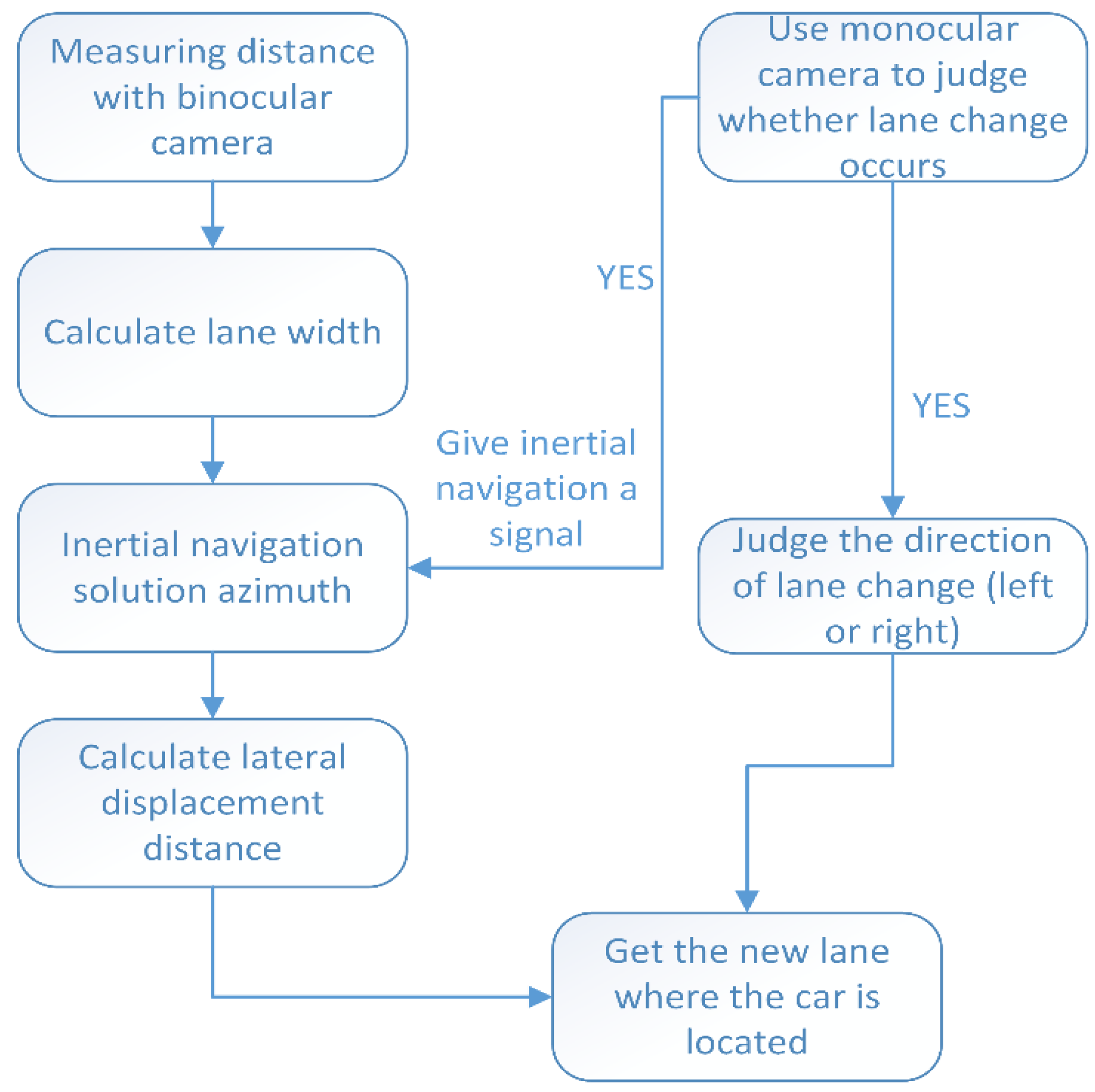
2.2. Vehicle Lateral Positioning Algorithm

Assume that the angular difference of the heading angle in adjacent time is α, and the gyroscope sampling frequency is 50 Hz. Since the steering phase is a uniform rotation, we divide the angle of the vehicle in the sampling interval of 0.02 s into 10 more parts to obtain a more accurate steering lateral distance S0, and the calculation process is shown in Equations (13)–(17).

$$S{0}_1={\displaystyle {\sum }_{k=1}^{10}\sin (\frac{{\alpha }_1}{10}\times k)}\times \frac{S{0}_{1(od)}}{10}$$

(13)

In the above formula, ${\alpha }_1$ is the amount of change in the heading angle of the car in the first 0.02 s, ${S0}_{1\left(od\right)}$ is the distance traveled in the first 0.02 s time, which can be obtained by the odometer, and ${S0}_2$ can be obtained by the same reasoning, as shown in the following equation:

$$S{0}_2={\displaystyle {\sum }_{k=1}^{10}\sin ({\alpha }_1+\frac{{\alpha }_2}{10}\times k)\times \frac{S{0}_{2(od)}}{10}}$$

(14)

The ${\alpha }_2$ in the above equation is the amount of change in the vehicle’s heading angle in the second 0.02 s, and so on to obtain ${S0}_n$.

$$S{0}_n={\displaystyle {\sum }_{k=1}^{10}\sin ({\alpha }_1+{\alpha }_2+\cdots \cdots +{\alpha }_{n-1}+\frac{{\alpha }_n}{10}\times k)\times \frac{S{0}_{n(od)}}{10}}$$

(15)

Adding ${S0}_1$, ${S0}_2$ …… ${S0}_n$ to obtain $S0$.

$$S0={\sum }_{i=1}^{n}S{0}_i$$

(16)

In the equation $n=\frac{t_0}{0.02}$, $t_0$ is the steering time.

The lateral distance S1 traveled during the holding phase is shown in the following equation:

$$S1=S{1}_{(od)}\times \sin \theta$$

(17)

In the above equation, ${S1}_{\left(od\right)}$ is the distance traveled by car in the holding phase, which can be obtained from the odometer, and θ is the difference between the heading angle at the beginning and end of the steering phase, ${\theta =\alpha }_1{+\alpha }_2+\cdots \cdots {+\alpha }_n$. The calculation of the lateral distance S2 in the return phase is the same as that of S0.

We have to set a threshold value for the steering angle of the vehicle at different speeds and determine whether the vehicle is changing lanes by the relationship between the difference of the heading angle in adjacent time and the threshold value. As shown in Figure 3, it is the maximum steering speed corresponding to different front wheel turning angles when the car is driving on roads with different adhesion coefficients. The tunnel is dry asphalt pavement, in general, the adhesion coefficient of good dry asphalt pavement is from 0.7 to 0.8. We take the median 0.75. According to Figure 3, taking into account the comfort of the driver in the car when changing lanes, we assume that the time of the car in the steering phase and the return phase is 0.2 s, and the sampling frequency of the inertial components is 50 Hz. We can obtain the front-wheel turning angle thresholds corresponding to different speeds of the car when changing lanes in the tunnel with 0.02 s as the unit time, as shown in

Table 1. Angular threshold for lane change at different speeds of the car.

Vehicle Speed $\mathit{v}$  $(\mathbf{m}/\mathbf{s})$	Front Wheel Steering Angle $(\mathbf{r}\mathbf{a}\mathbf{d})$	Angular Speed of Steering $(\mathbf{r}\mathbf{a}\mathbf{d}/\mathbf{s})$	Angular Threshold per Unit of Time $(\mathbf{r}\mathbf{a}\mathbf{d})$
$v \le 8.3$	0.175	0.875	0.0175
$8.3 < v \le 16.7$	0.122	0.611	0.0122
$16.7 < v \le 22.2$	0.087	0.436	0.0087

.

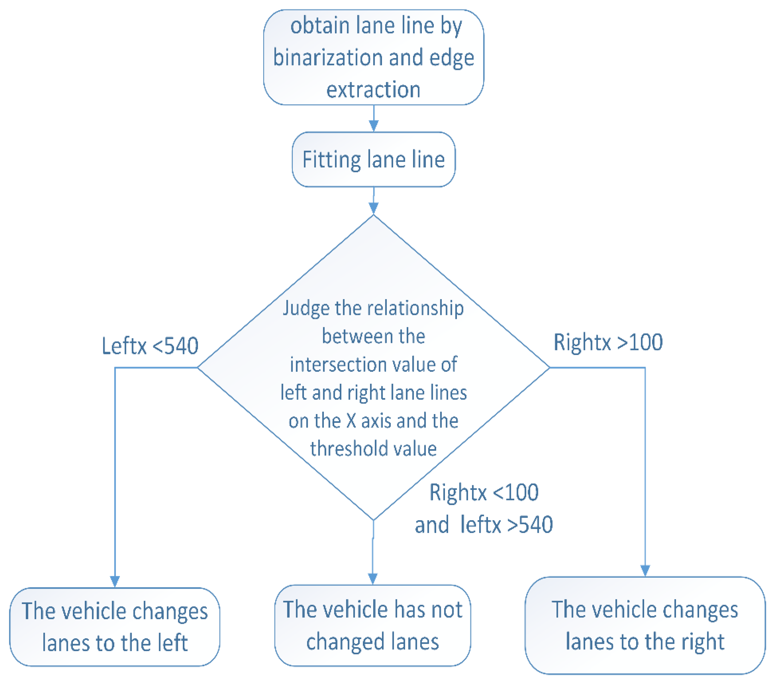
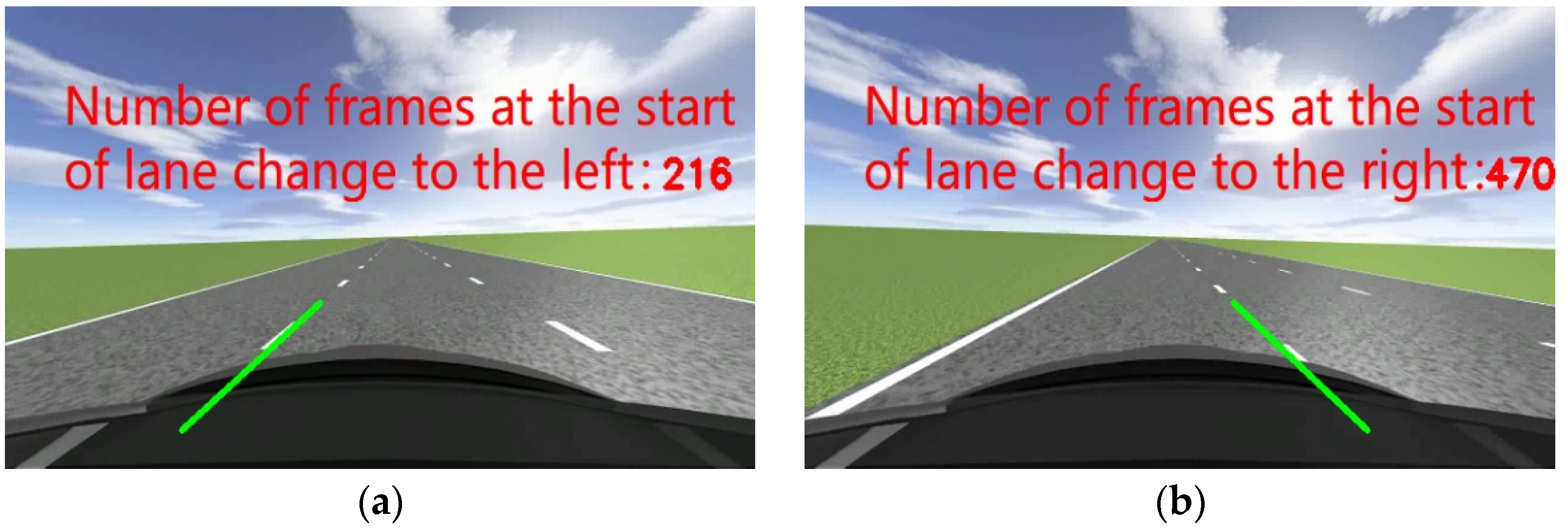
2.3. Monocular Camera to Assist in Determining Lane Changes

When there are some small obstacles in the lane where the vehicle is located, the vehicle needs to avoid them, as shown in Figure 4. In this case, the method of using the difference of adjacent time heading angles to determine the lane change as described above will be misjudged. Therefore, this paper proposes the use of monocular cameras to assist in determining whether a lane change occurs in a vehicle.

The monocular camera lane-changing algorithm in this paper is mainly based on the intersection value of lane lines on the x-axis to determine whether the vehicle is changing lane behavior. When the car changes lane to the left, the value of the intersection of the left lane line on the x-axis will become smaller, while the right lane line will gradually disappear due to the ROI region, as shown in Figure 5a. Therefore, to determine whether a car has changed lanes to the left is mainly by using the value of the intersection of the left lane line on the x-axis, and whether a right lane change has occurred is judged by using the value of the intersection of the right lane line on the x-axis. In order to obtain the appropriate threshold value of x-axis intersection, we carried out a real vehicle experiment in Jiaozhou Bay tunnel in Qingdao. The monocular camera is fixed in the center of the front windshield of the car to shoot the road, and the video is processed using OpenCV to obtain the lane lines and draw the fitted lane lines, as shown in Figure 5b.

In the test, the speed was 60 km/h. We first made a left lane change, kept the steering wheel still for some distance after the left lane change, and then made a right lane change.

We find the intersection values of the left and right fitted lane lines on the x-axis and input them into MATLAB for visualization, as shown in Figure 6.

From Figure 6 we can see that the left lane line has two valleys at the x-axis intersection value, while the right lane line has two peaks at the x-axis intersection, and these two distinct changes are generated at the beginning of the lane change. Combining the data in the figure, we take the threshold value of 540 for the left lane line at the x-axis intersection and 100 for the right lane line at the x-axis intersection. The flowchart of monocular camera-assisted lane change determination is shown in Figure 7.

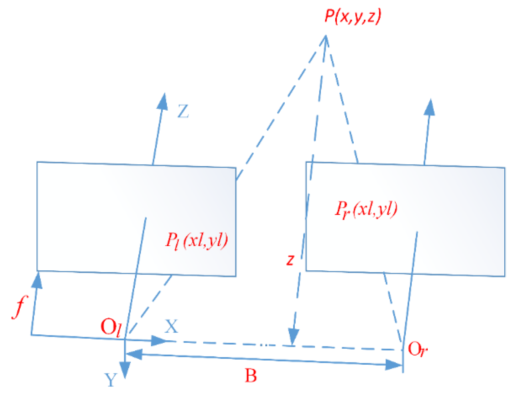
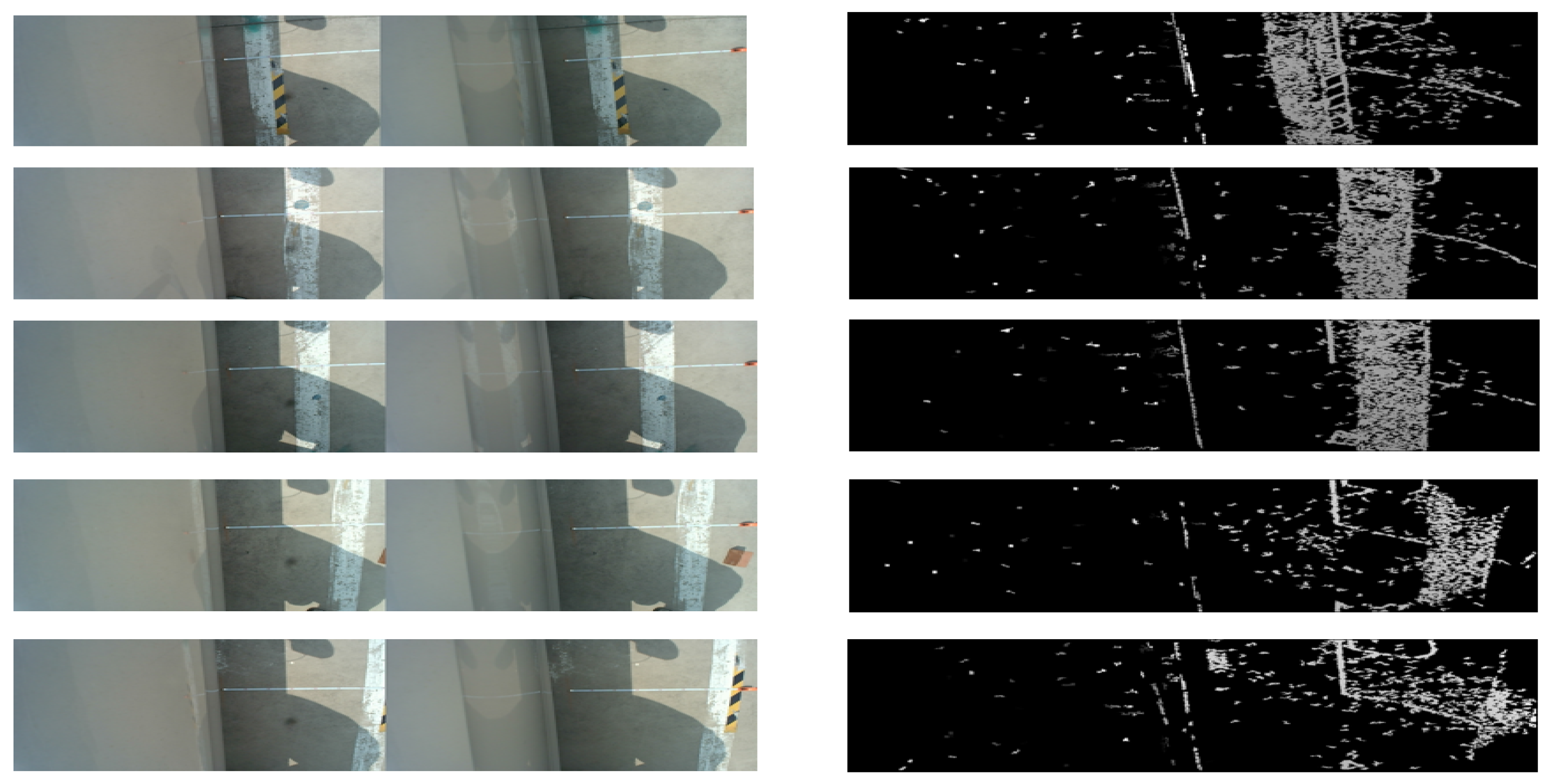
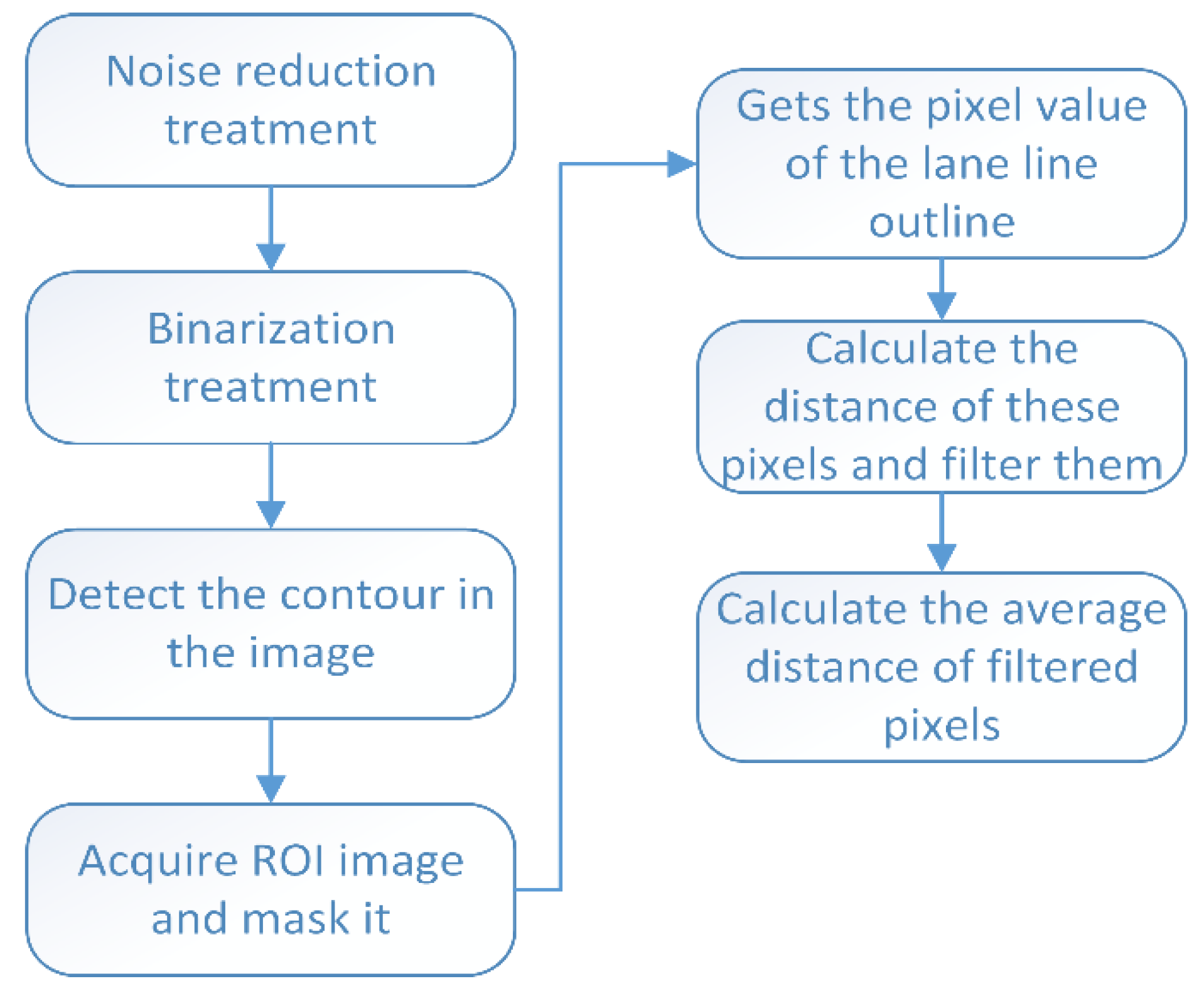
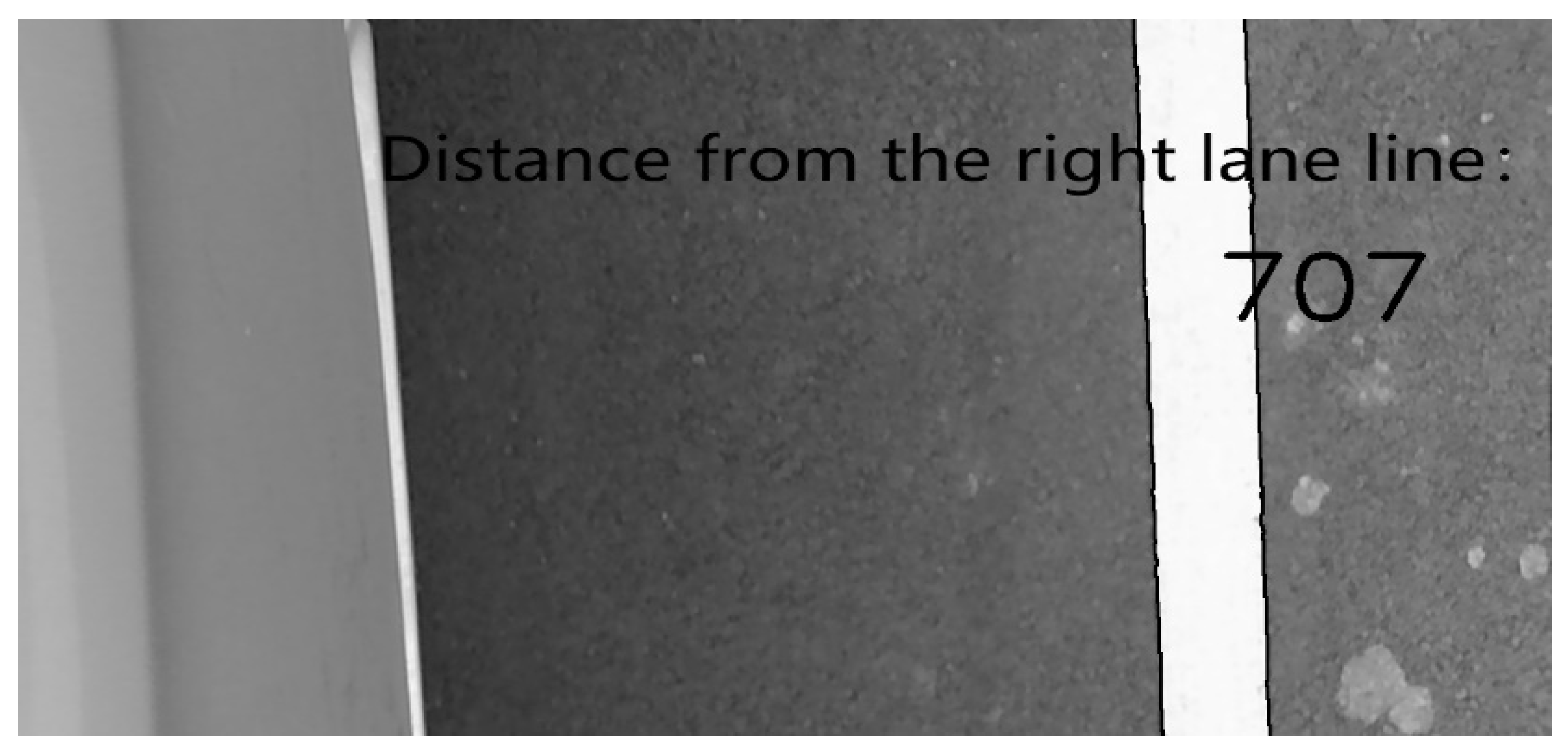
2.4. Binocular Camera Distance Measurement

In the previous section we have assumed that the lane width is 4.5 m, but for real road conditions, the lane width varies from road to road, so it is necessary to actually measure the lane width. The accuracy of the front monocular camera in measuring the lateral width is not enough, so this paper uses two binocular cameras fixed under the left and right rearview mirrors of the vehicle to measure the distance between the two sides of the vehicle from the lane line, and then measure the distance between the two cameras under the left and right rearview mirrors to find out the lane width. The basic principle of binocular camera stereo vision is to use two cameras to complete binocular image acquisition of the target in front of the lens. Due to the difference in the shooting angle and position of the left and right cameras for image acquisition, there is a certain parallax between the two images of the target object acquired by the two cameras at the same moment, and the spatial coordinates of the target object are derived based on the parallax [25]. The binocular vision ranging model is shown in Figure 8.

In the Figure 8, $O_l$, and $O_r$ are the optical center positions of the two cameras. The length of the line between $O_l$ and $O_r$ is the baseline distance B, Z is the optical axis of the left camera, the left and right cameras are parallel to each other. If there is a point $P(x,y,z)$ in space, the projection points on the left and right camera images are $P_l{(x}_l{,y}_l)$ and $P_r{(x}_r{,y}_r)$. When the left and right cameras are mounted ideally, then we have $y_l=y_r=y^{’}$. The following equation can be derived from similar triangles:

$$\{\begin{array}{c}{x}_l=f\frac{x}{z}\\ x_r=f\frac{B-x}{z}\\ y^{\prime }=f\frac{y}{z}\end{array}$$

(18)

By transforming the above equation, it is possible to derive the coordinate equation that can solve for the point P in space.

$$\{\begin{array}{c}x=\frac{B\cdot x_l}{x_l-x_r}=\frac{B\cdot x_l}{D}\\ y=\frac{B\cdot y^{\prime }}{x_l-x_r}=\frac{B\cdot y^{\prime }}{D}\\ Z=\frac{B\cdot f}{x_l-x_r}=\frac{B\cdot f}{D}\end{array}$$

(19)

In the above equation, ${D=x}_l-x_r$, is called the parallax of the two images captured by the left and right cameras. The above equation shows that to find the coordinates of a spatial point using a binocular camera requires the baseline distance B of the left and right cameras, the parallax D of the left and right images, and the focal length f of the camera. B and f are derived from the calibration of the camera, and in this paper the binocular camera is calibrated using the Zhengyou Zhang calibration method [26]. Parallax D is obtained by stereo matching, and this paper uses the Block Matching (BM) algorithm that comes with OpenCV to perform stereo matching, which has the advantage that the algorithm is fast, which meets our requirement of using it on a moving vehicle.

3. Results

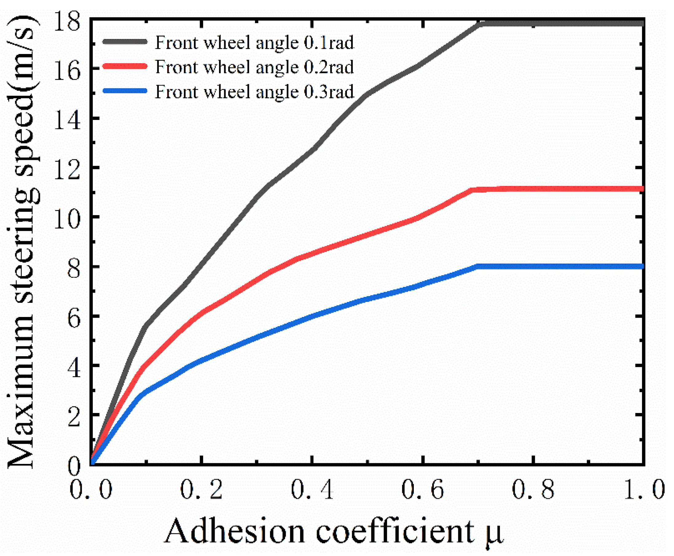
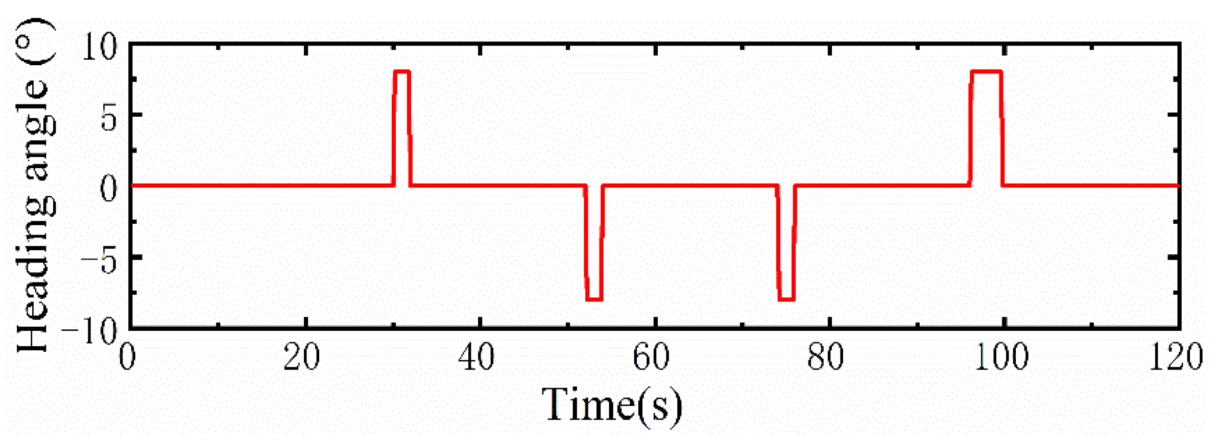
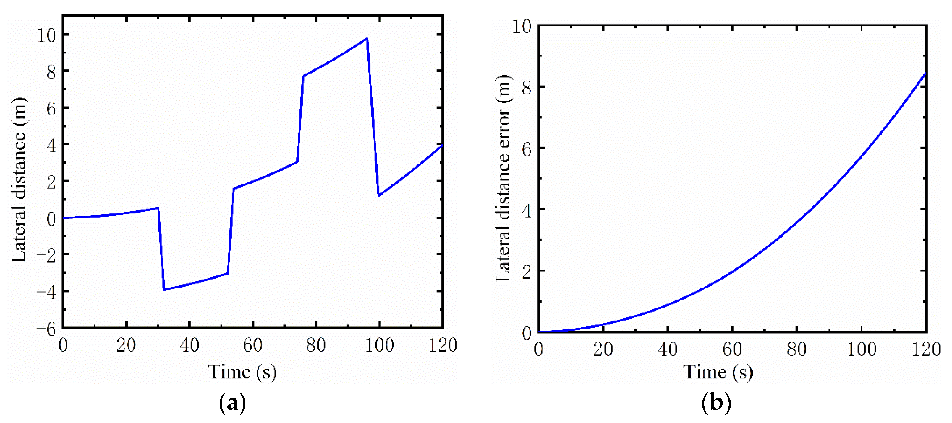
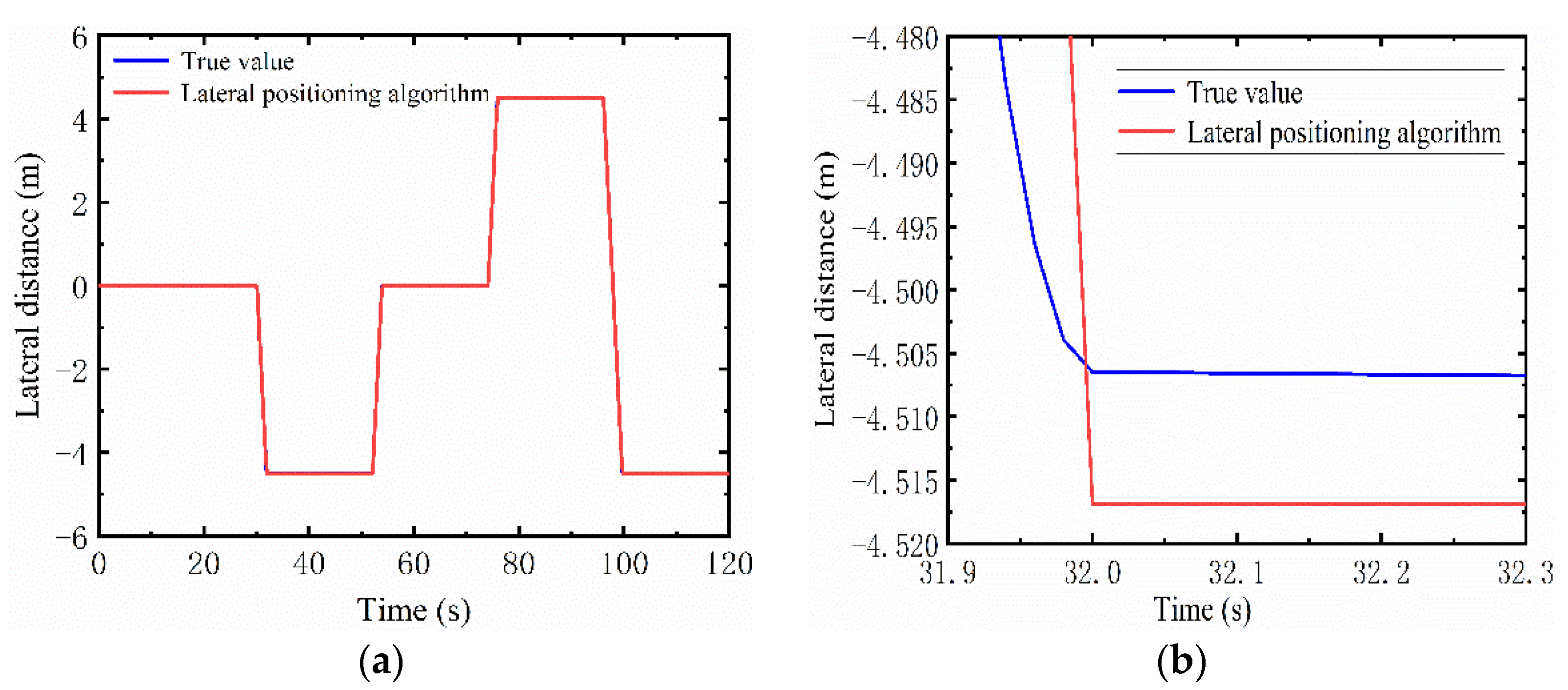
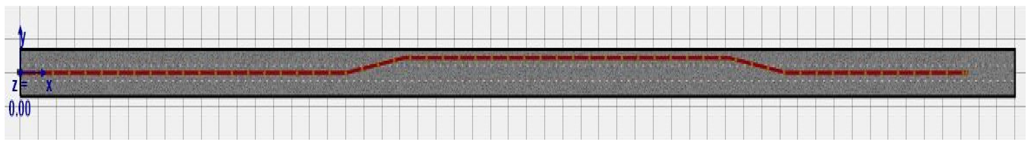
3.1. Simulation Analysis of Lateral Positioning Algorithm

A trajectory of a car running from south to north is obtained by trajectory simulation using MATLAB, and the inertial device output information is obtained by using the backpropagation method. Assuming a lane width of 4.5 m and a total of three lanes, the vehicle enters the tunnel at the center of the middle lane. As shown in Figure 9a, the simulation diagram of the vehicle’s trajectory, the distance to the change lane to the right is positive, and the distance to the change lane to the left is negative. The working conditions include the following four states: changing lanes to the left, changing lanes to the right, changing two lanes to the left, and driving in a straight line. The car travels at a speed of 18 m/s (about 65 km/h), and the car turns at an angle of 8° each time it changes lane, and the angular speed when turning is 40°/s. From this, the real-time lateral distance of the car while driving can be obtained, as shown in Figure 9b.

MATLAB is used to simulate the pure inertial guidance solution, setting the bias of the gyroscope and accelerometer in strapdown inertial guidance to 0.1 deg/h and 100 µg respectively, and the noise of the gyroscope and accelerometer to 0.01 deg/sqrt (h) and 10 µg/sqrt (Hz) respectively, and the sampling frequency of inertial components is 50 Hz. The initial position error of latitude and longitude height is 1 m. The initial azimuth error is set to 0.5 arc second for the east and north directions, the speed error is 0 m/s, the time delay between the odometer data and IMU data is 0 s, and the odometer scale factor error is set to 1. Figure 10 shows the vehicle heading angle variation, Figure 11a shows the lateral distance variation under the inertial guidance solution, and Figure 11b shows the error of the lateral distance from the inertial guidance solution. It can be seen from Figure 11b that the error of vehicle lateral displacement distance solved by inertial navigation increases with the increase in time, which is in line with the characteristics of inertial navigation’s positioning error accumulated with time, and the error is close to 9 m in about 120 s, which obviously does not meet the requirements of vehicle lateral positioning.

As shown in Figure 12, it is a graph of the change in vehicle lateral distance based on the algorithm proposed in this paper. From Figure 12, it can be seen that the vehicle lateral distance solved based on the algorithm in this paper is basically consistent with the real distance, and the two data lines basically overlap. Figure 13 shows the error of the lateral distance of the vehicle based on the algorithm of this paper, with a maximum error of about 0.13 m. Since the four error peaks have typical coarse error characteristics and are generated during the lane change process, they can be eliminated in the actual system. For the whole process of lane change, the difference between the calculated distance and the real distance is less than 0.02 m at the end of the lane change (Figure 12b). It can be seen that when the accuracy of inertial components is not high, the algorithm proposed in this paper can still provide high positioning accuracy, so the algorithm has good robustness in practical applications and is less affected by the accuracy error of inertial components, which has high practicality.

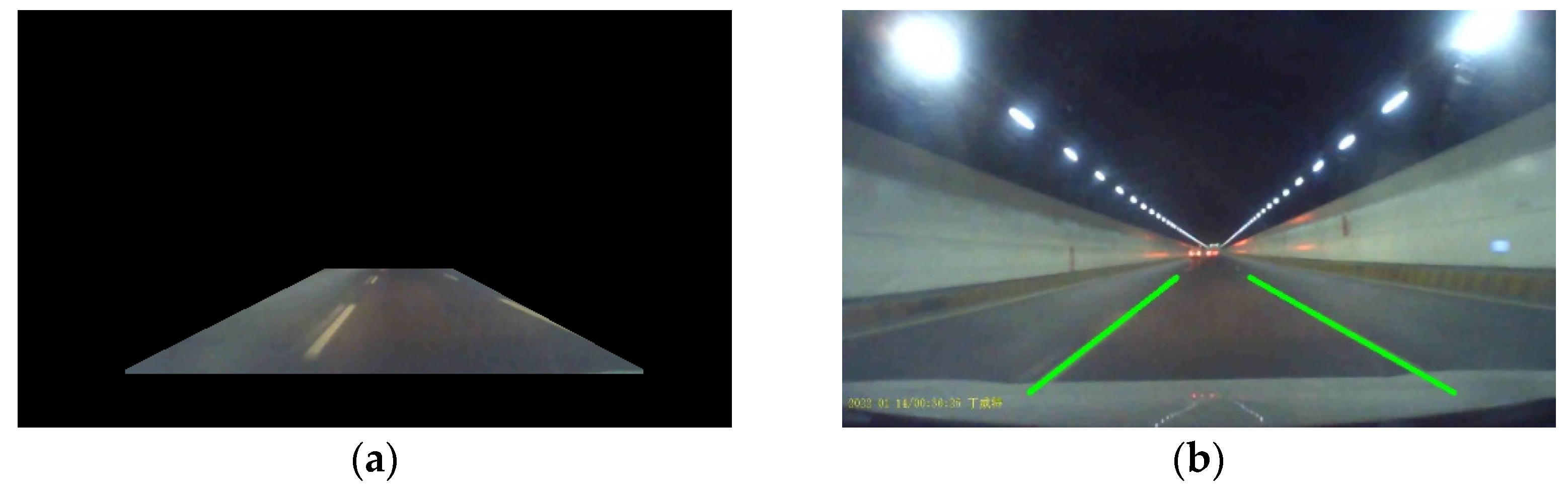
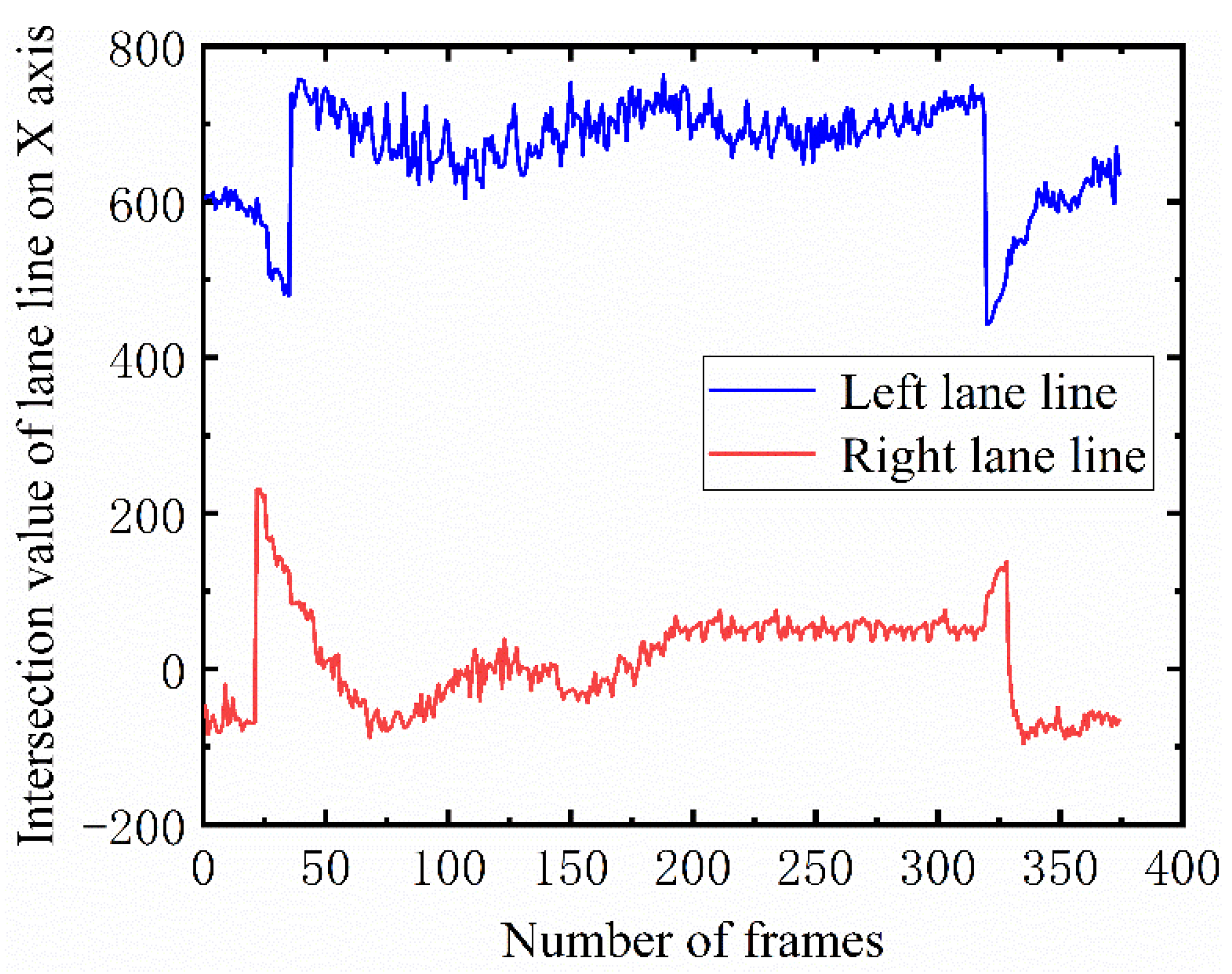
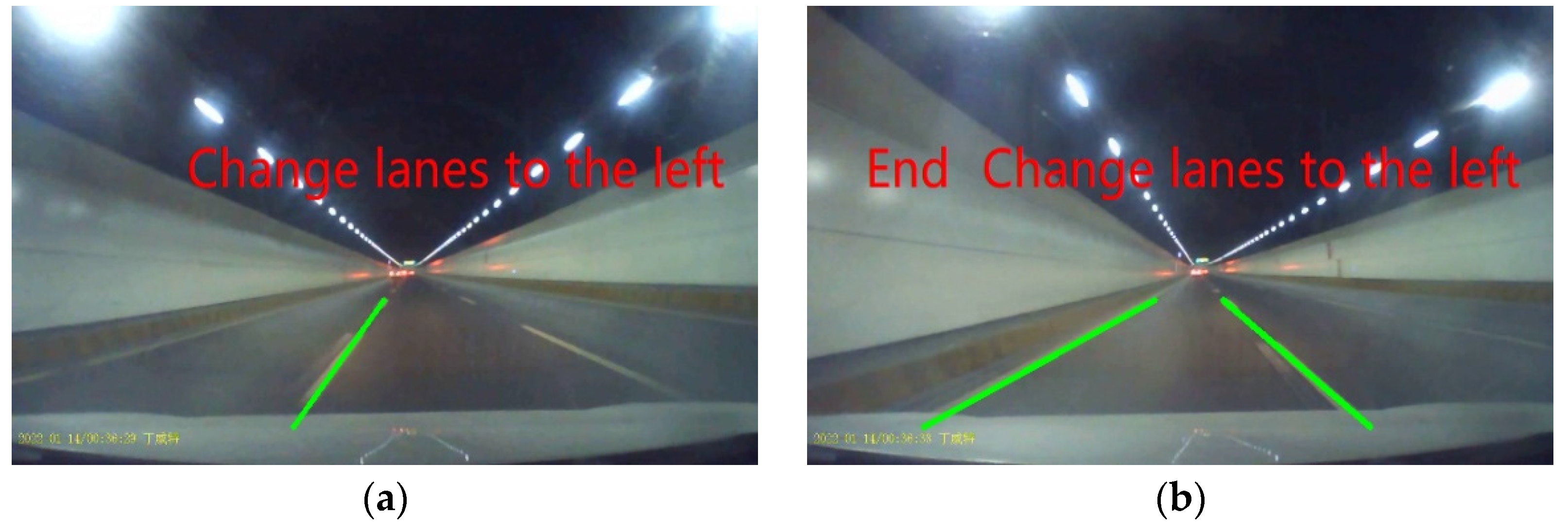
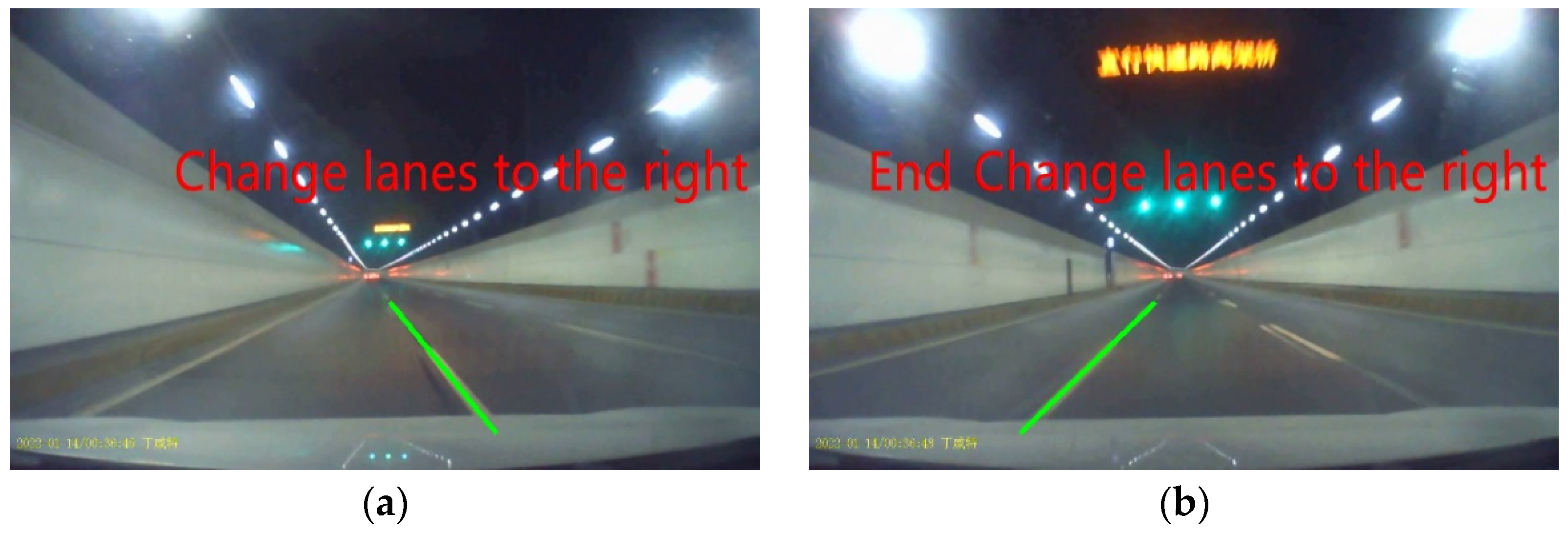
3.2. Simulation of Monocular Camera Lane Change Judgment

We put the video taken from the real car into OpenCV for simulation, the results of the simulation are shown in Figure 14 and Figure 15.

From Figure 14 and Figure 15, the monocular camera can be a good aid to determining whether the vehicle is changing lanes, but the lane change judgment of the monocular camera will have a lag, and the moment of lane change is judged by the lane line intersection is often later than the real start moment of the lane change. In order to find out the lag time of the monocular camera lane change judgment, we simulated a section of car motion trajectory in the simulation software Prescan to obtain the exact lane change time point of the vehicle. Then the vehicle driving video is processed in OpenCV to obtain the start moment of the lane change judged by the monocular camera, and the lag time can be found by comparing the two moments. Create a road in Prescan and give the vehicle a driving trajectory as shown in Figure 16 and Figure 17, where the width of each lane is 4.5 m and the initial speed of the vehicle is 18 m/s and is kept at a constant speed. The difference in heading angle for each lane change of the car is $8^{°}$. The vehicle made two lane changes while driving, one to the left at 10 s and one to the right at 21.8 s. The simulation in OpenCV determines the start of a lane change by the number of frames in the video, with a frame rate of 20 frames per second.

The moment when the vehicle starts to change lanes, as determined by the monocular camera simulated in OpenCV, is shown in Figure 18.

Through the above data we can obtain the difference between the two times, the specific results are shown in

Table 2. Lag time of monocular camera lane change judgment.

	Real Time (s)	Time of Monocular Camera Judgment (Frame)	Time Difference (s)
First lane change	10	216	0.8
Second lane change	21.8	470	1.7

.

From Table 2, we can see that the difference between the moment judged by the monocular camera and the real moment during the second lane change is even larger at 1.7 s. Thus, we set the lag time to 2 s. When the difference in the heading angle of the vehicle within the adjacent time is greater than the threshold value, the lateral displacement of the vehicle is calculated based on the lateral positioning algorithm at this time first, and the lateral displacement calculation of the vehicle takes effect when the vehicle receives the lane change signal from the monocular camera within 2 s; otherwise, the vehicle is deemed not to have changed lanes.

The simulation and experiment of the monocular camera mentioned above are aimed at the case where the lane width is 4.5 m. We found that the lane widths in different tunnels in China have the following different widths: 3 m, 3.5 m, 4 m, and 4.5 m, respectively. In order to make the system more applicable, we take the threshold value of the intersection point for the lanes with different widths. The results of the thresholds are shown in the

Table 3. Threshold value of intersection at different lane widths.

Lane Width (m)	Threshold Value of Intersection Point of Left Lane Line on x-axis during Left Lane Change	Threshold Value of Intersection Point of Right Lane Line on x-axis during Right Lane Change
3	480	150
3.5	500	130
4	520	115

.

We conducted a simulation test of lane change judgment with a monocular camera for lanes of different widths. The specific test results are shown in the figure below.

It can be seen from Figure 19 that after selecting different intersection thresholds for different lanes, the monocular camera can well judge whether vehicles change lanes at different widths, which makes the monocular camera’s lane change judgment algorithm more applicable. From the right half of the above figure, we can see that the lane change judgment of the monocular camera is less affected by the light intensity. We still need to obtain the delay time of monocular camera lane change judgment at different lane widths. Figure 19 gives the lane change start time judged by the camera. The specific results are shown in

Table 4. Lag time for different lane widths.

Lane Width (m)	The Real Time of the First Lane Change (s)	The First Lane Change Time Judged by Monocular Camera (Frame)	The Real Time of the Second Lane Change (s)	The Second Lane Change Time Judged by Monocular Camera (Frame)	First Lag Time (s)	Second Lag Time (s)
3	10	216	22.4	455	0.8	0.35
3.5	10	221	22.7	455	1.05	0.05
4	10	221	23.2	464	1.05	0

.

From Table 4, we can see that when the lane width is different, the delay time of the monocular camera lane change judgment is less than 2 s. Therefore, it is reasonable to set the delay time to 2 s as proposed in the previous article, which also proves the rationality of the thresholds proposed in Table 3.

3.3. Simulation and Experiment of Binocular Camera Range Measurement

First, we fixed the binocular camera under the rearview mirror of the vehicle to take pictures of the lane line and conducted five sets of static ranging experiments for binocular camera ranging, taking pictures of the lane line and measuring the distance when the vehicle was stationary and parked next to the lane line. The results are shown in

Table 5. Static distance measurement experiment data of binocular camera.

Serial Number	Actual Distance (mm)	Measuring Distance of Binocular Camera (mm)	Error (mm)
1	159	163	4
2	339	330	9
3	342	345	3
4	522	529	7
5	670	651	19

; the experimental diagram is shown in Figure 20. In Figure 20, the left side is the image taken by the binocular camera, and the right side is the parallax image.

It can be seen from Figure 20 that the parallax map is less effective when the vehicle is 670 mm away from the lane line. The main reason why the lane line in the parallax map cannot be clearly distinguished is the illumination, but the error is still within an acceptable range, so it is feasible to measure the distance between the vehicle and the lane line using a binocular camera mounted under the vehicle’s rearview mirror and calculate the lane width from it.

When the vehicle is moving, we need to dynamically measure the distance between the vehicle and the lane line. For static distance measurement, the pixel points in the lane lines are manually selected by us. For dynamic distance measurement, we need to do some processing to obtain the pixel points in the lane lines. In this paper, the origin of coordinates used for distance measurement by the binocular camera are all based on the optical center of the left camera, so all image processing is performed for the left image in the binocular camera. Firstly, the image should be processed for noise reduction, then the image should be binarized and the contours in the image should be detected, the image should be ROI processed and masked, the purpose of doing so is to remove the influence of the vehicle contour lines, then the distance of the contour points of the lane line should be calculated and screened to remove some obviously unreasonable distance values, and finally the average value of these values should be calculated as the distance of the vehicle from the lane line, the specific process is shown in Figure 21.

According to the dynamic distance measurement process described in the previous section, we conducted a real-world experiment in which we mounted a binocular camera under the right side mirror of the vehicle to take pictures of the lane lines while the vehicle was moving. Considering that the lane lines taken by the left camera were already incomplete when the vehicle was 67 cm away from the lane lines in the static experiment, we reinstalled and re-calibrated the binocular camera. The video shot by the binocular camera is put into OpenCV for processing. Figure 22a shows the contour image of the lane line, Figure 22b shows the parallax image of the lane line, and Figure 23 shows the distance between the left camera and the right lane line measured by the binocular camera under vehicle dynamics, the unit of distance is millimeters.

It can be seen from Figure 22a that the contour of the lane line is well extracted, and from Figure 22b the contour of the lane line can be clearly distinguished. Compared with static distance measurement, the difficulty of dynamic distance measurement lies in the extraction of pixels from lane lines. We extract the edge contours of lane lines by the contour extraction method, but since the BM algorithm searches for strong matching (strong texture) between two images, it cannot accurately calculate the depth of pixels on some lane contours, so we cannot accurately obtain the distance between these pixels and the camera in the world coordinates. Therefore, we screened these pixels and obtained those pixels with a reasonable distance. It can be seen from Figure 23 that the measured distance is still reasonable when the vehicle is moving dynamically, which proves the effectiveness of the dynamic distance measurement proposed in this paper.

4. Discussion and Conclusions

In this paper, a vehicle positioning system combining a monocular camera, a binocular camera, and inertial navigation is proposed to solve the problem of GPS lock-out in a long tunnel. In the absence of a GPS signal, when a vehicle changes lanes or overtakes, the system can provide high-precision vehicle lateral positioning and accurately obtain the lane where the vehicle is after a lane change or overtaking. The traditional inertial navigation positioning algorithm is greatly affected by the accuracy of inertial components, and the error will increase with the accumulation of time. The high-precision inertial components will increase the cost of the system, which is one of the reasons why the current inertial navigation is still not popular. In this paper, the vehicle lateral positioning algorithm based on the heading angle calculated by inertial navigation has high lateral positioning accuracy and is less affected by inertial components. The positioning error will not increase with the accumulation of time, which can reduce the cost of the positioning system and has good engineering application value. With the help of a binocular camera and a monocular camera, the system has better anti-interference. When the vehicle is in a congested or low-speed section in the tunnel, the monocular camera may fail to recognize the lane line due to the obstruction of the vehicle in front. At this time, the binocular camera can be used to measure the distance between the vehicle and the lane line, judge whether the vehicle keeps driving in the lane, and assist in judging whether the vehicle changes lanes according to the distance information; therefore, the system also has good robustness.

References

1. Li, H.; Xu, Q. A Reliable Fusion Positioning Strategy for Land Vehicles in GPS-Denied Environments Based on Low-Cost Sensors. IEEE Trans. Ind. Electron. 2017, 64, 3205–3215. [Google Scholar] [CrossRef]
2. Elsheikh, M.; Noureldin, A.; El-Sheimy, N.; Korenberg, M. Performance Analysis of MEMS-based RISS/PPP Integrated Positioning for Land Vehicles. In Proceedings of the 2020 IEEE 92nd Vehicular Technology Conference (VTC2020-Fall), Victoria, BC, Canada, 18 November–16 December 2020; pp. 1–5. [Google Scholar] [CrossRef]
3. Zheng, C.; Libo, C.; Linbo, Y.; Qin, Q.; Ruifeng, Z. Lane-level positioning system based on RFID and vision. In Proceedings of the IET International Conference on Intelligent and Connected Vehicles (ICV 2016), Chongqing, China, 22–23 September 2016; pp. 1–5. [Google Scholar] [CrossRef]
4. Wei, S.; Zou, Y.; Zhang, X.; Zhang, T.; Li, X. An Integrated Longitudinal and Lateral Vehicle Following Control System with Radar and Vehicle-to-Vehicle Communication. IEEE Trans. Veh. Technol. 2019, 68, 1116–1127. [Google Scholar] [CrossRef]
5. Chen, H.; Taha, T.M.; Chodavarapu, V.P. Towards Improved Inertial Navigation by Reducing Errors Using Deep Learning Methodology. Appl. Sci. 2022, 12, 3645. [Google Scholar] [CrossRef]
6. Tang, J.; Zhang, Y.; Li, A. Research on Location Method Based on GNSS/IMU/LIDAR Multi-source Information Fusion. In Proceedings of the 2021 3rd International Conference on Intelligent Control, Measurement and Signal Processing and Intelligent Oil Field (ICMSP), Xi’an, China, 23–25 July 2021; pp. 98–102. [Google Scholar]
7. Song, D.; Tian, G.-M.; Liu, J. Real-time localization measure and perception detection using multi-sensor fusion for Automated Guided Vehicles. In Proceedings of the 2021 40th Chinese Control Conference (CCC), Shanghai, China, 26–28 July 2021; pp. 3219–3224. [Google Scholar] [CrossRef]
8. Pan, L.; Ji, K.; Zhao, J. Tightly-Coupled Multi-Sensor Fusion for Localization with LiDAR Feature Maps. In Proceedings of the 2021 IEEE International Conference on Robotics and Automation (ICRA), Xi’an, China, 30 May–5 June 2021; pp. 5215–5221. [Google Scholar] [CrossRef]
9. Alrousan, Q.; Matta, S.; Tasky, T. Multi-Sensor Fusion in Slow Lanes for Lane Keep Assist System; SAE Technical Paper 2021-01-0084; SAE International: Warrendale, PA, USA, 2021. [Google Scholar] [CrossRef]
10. Qian, H.; An, D.; Xia, Q. IMM-UKF based land-vehicle navigation with low-cost GPS/INS. In Proceedings of the 2010 IEEE International Conference on Information and Automation, Harbin, China, 20–23 June 2010; pp. 2031–2035. [Google Scholar] [CrossRef]
11. Zhu, X.; Tian, W.; Li, G.; Yu, J. Research on Localization Vehicle Based on Multiple Sensors Fusion System. In Proceedings of the 2017 International Conference on Computer Network, Electronic and Automation (ICCNEA), Xi’an, China, 23–25 September 2017; pp. 491–494. [Google Scholar] [CrossRef]
12. Yang, B.; Xue, L.; Fan, H.; Yanga, X. SINS/Odometer/Doppler Radar High-Precision Integrated Navigation Method for Land Vehicle. IEEE Sens. J. 2021, 21, 15090–15100. [Google Scholar] [CrossRef]
13. Serov, A.; Clemens, J.; Schill, K. Visual-Multi-Sensor Odometry with Application in Autonomous Driving. In Proceedings of the 2021 IEEE 93rd Vehicular Technology Conference (VTC2021-Spring), Helsinki, Finland, 25–28 April 2021; pp. 1–7. [Google Scholar] [CrossRef]
14. Wang, F.; Duan, J.-M.; Zheng, B.-G. Machine vision based localization of intelligent vehicle. In Proceedings of the 10th World Congress on Intelligent Control and Automation, Beijing, China, 6–8 July 2012; pp. 4638–4643. [Google Scholar] [CrossRef]
15. Bai, X.; Wu, C.; Hou, Q.; Feng, D. Vehicle Precise Positioning Based on Integrated Navigation System in Vehicle Networking. In Proceedings of the 2021 IEEE International Conference on Robotics, Automation and Artificial Intelligence (RAAI), Hong Kong, China, 21–23 April 2021; pp. 48–52. [Google Scholar] [CrossRef]
16. Li, K.; Ouyang, Z.; Hu, L.; Hao, D.; Kneip, L. Robust SRIF-based LiDAR-IMU Localization for Autonomous Vehicles. In Proceedings of the 2021 IEEE International Conference on Robotics and Automation (ICRA), Xi’an, China, 30 May–5 June 2021; pp. 5381–5387. [Google Scholar]
17. Zhang, Z.; Zhao, J.; Huang, C.; Li, L. Learning Visual Semantic Map-Matching for Loosely Multi-sensor Fusion Localization of Autonomous Vehicles. IEEE Trans. Intell. Veh. 2022. [Google Scholar] [CrossRef]
18. Yu, L.; Jie, L.; Haoru, L.; Sijia, L. Large-scale scene mapping and localization based on multi-sensor fusion. In Proceedings of the 2021 6th International Conference on Intelligent Computing and Signal Processing (ICSP), Xi’an, China, 9–11 April 2021; pp. 1130–1135. [Google Scholar] [CrossRef]
19. Chen, J.; Zhang, Q.; Pan, J.; Liang, J. A vehicle autonomous positioning technology based on terrain relative navigation. In Proceedings of the 2021 China Automation Congress (CAC), Beijing, China, 22–24 October 2021; pp. 6737–6740. [Google Scholar] [CrossRef]
20. Liu, B.; Liu, G.; Wei, S.; Su, G.; Wang, J. On Improved Algorithm of SINS/DR Integrated Navigation System. In Proceedings of the 2018 IEEE CSAA Guidance, Navigation and Control Conference (CGNCC), Xiamen, China, 10–12 August 2018; pp. 1–6. [Google Scholar] [CrossRef]
21. Zhao, Y.; Yang, Z.; Song, C.; Xiong, D. Vehicle dynamic model-based integrated navigation system for land vehicles. In Proceedings of the 2018 25th Saint Petersburg International Conference on Integrated Navigation Systems (ICINS), St. Petersburg, Russia, 28–30 May 2018; pp. 1–4. [Google Scholar] [CrossRef]
22. Vigrahala, J.; Ramesh, N.V.K.; Devanaboyina, V.R.; Reddy, B.N.K. Attitude, Position and Velocity determination using Low-cost Inertial Measurement Unit for Global Navigation Satellite System Outages. In Proceedings of the 2021 10th IEEE International Conference on Communication Systems and Network Technologies (CSNT), Bhopal, India, 18–19 June 2021; pp. 61–65. [Google Scholar] [CrossRef]
23. Abosekeen, A.; Noureldin, A.; Korenberg, M.J. Improving the RISS/GNSS Land-Vehicles Integrated Navigation System Using Magnetic Azimuth Updates. IEEE Trans. Intell. Transp. Syst. 2020, 21, 1250–1263. [Google Scholar] [CrossRef]
24. Jiang, Y.F.; Lin, Y.P. Error analysis of quaternion transformations (inertial navigation). IEEE Trans. Aerosp. Electron. Syst. 1991, 27, 634–639. [Google Scholar] [CrossRef]
25. Yaping, Z.; Zhihang, S. Research on Binocular Forest Fire Source Location and Ranging System. In Proceedings of the 2020 IEEE International Conference on Power, Intelligent Computing and Systems (ICPICS), Shenyang, China, 28–30 July 2020; pp. 199–202. [Google Scholar] [CrossRef]
26. Zhang, Z. A flexible new technique for camera calibration. IEEE Trans. Pattern Anal. Mach. Intell. 2000, 22, 1330–1334. [Google Scholar] [CrossRef] [Green Version]
Figure 1. Vehicle lateral positioning system.
Applsci 12 06634 g001
Figure 2. Vehicle lane change diagram.
Applsci 12 06634 g002
Figure 3. Maximum steering speed for different front wheel angles.
Applsci 12 06634 g003
Figure 4. Vehicle avoidance obstacle schematic.
Applsci 12 06634 g004
Figure 5. Actual photo of lane in tunnel: (a) Vehicle ROI figure; (b) Lane Line Fitting Diagram.
Applsci 12 06634 g005
Figure 6. Value of the intersection of the left and right lane lines on the x-axis.
Applsci 12 06634 g006
Figure 7. Flow chart of monocular camera lane change judgment.
Applsci 12 06634 g007
Figure 8. Model for distance measurement by binocular camera.
Applsci 12 06634 g008
Figure 9. Vehicle track information image: (a) Vehicle track information; (b) Lateral distance variation of the vehicle.
Applsci 12 06634 g009
Figure 10. Vehicle heading angle information.
Applsci 12 06634 g010
Figure 11. Inertial guidance solution information: (a) Lateral distance variation of the inertial guidance solution; (b) Lateral distance error of inertial guidance solution.
Applsci 12 06634 g011
Figure 12. Lateral distance variation based on the algorithm of this paper: (a) Lateral distance variation of vehicles based on lateral positioning algorithm; (b) Local enlargement.
Applsci 12 06634 g012
Figure 13. Error of the lateral positioning algorithm.
Applsci 12 06634 g013
Figure 14. Images of the start and end moments of the vehicle lane change to the left: (a) Image of the start moment of the vehicle lane change to the left; (b) Image of the end moment of the vehicle lane change to the left.
Applsci 12 06634 g014
Figure 15. Images of the start and end moments of the vehicle lane change to the right: (a) Image of the start moment of the vehicle lane change to the right; (b) Image of the end moment of the vehicle lane change to the right.
Applsci 12 06634 g015
Figure 16. Vehicle track information.
Applsci 12 06634 g016
Figure 17. Vehicle track images.
Applsci 12 06634 g017
Figure 18. The start moment of the vehicle changing lane to the left and to the right as judged by the monocular camera: (a) The moment when the vehicle starts to change lanes to the left; (b) The moment when the vehicle starts to change lanes to the right.
Applsci 12 06634 g018
Figure 19. Lane changing judgment of monocular camera with different lane widths.
Applsci 12 06634 g019
Figure 20. Experimental diagram of binocular camera static distance measurement.
Applsci 12 06634 g020
Figure 21. Flow chart of dynamic distance measurement using binocular camera.
Applsci 12 06634 g021
Figure 22. Lane line image after processing: (a) Contour image of the lane line; (b) Parallax image of lane lines.
Applsci 12 06634 g022
Figure 23. Distance between vehicle and lane line measured by binocular camera when driving.
Applsci 12 06634 g023