1. Introduction
Object detection is a computer technology related to computer vision and image processing that aims to determine and detect many target objects from still images or video data [
1]. It widely comprises different important techniques, namely image processing, pattern recognition, artificial intelligence (AI), and machine learning (ML). It finds applicability in different domains such as road traffic accident prevention, theft detection, traffic management, etc. [
2,
3]. Intelligent video surveillance is a vintage subject in the domain of image processing and computer vision that has recently become well known. It has numerous significant benefits, such as accurate data processing, low human resource cost, and effective information gathering organization [
4]. Crowd density estimation is regarded as a significant application in visual surveillance, and it plays an important role in crowd management and monitoring. Specifically for service providers in public areas, a crowd density estimation system could show how many consumers are currently waiting and therefore provide an appropriate reference to send the bounded sources reasonably and effectively [
5].
Crowd density estimation refers to the assessment of crowd dispersal and the particular number of people [
6]. Crowd analysis has attracted substantial interest among researchers in recent years because of various reasons. The massive increase in the global population and in urbanization has resulted in an increase in such events as public demonstrations, sporting events, political rallies, and so on. Similar to other computer vision issues, crowd analysis faces numerous difficulties, such as inter-scene variations in appearance, occlusions, uneven distribution of people, high clutter, intra-scene and scale issues, non-uniform illumination, and an unclear viewpoint; these problems are immensely difficult to solve [
7,
8]. The perplexity of the issue along with the extensive array of applications for crowd analysis has led to an increased focus among research scholars in recent years.
Convolutional neural network (CNN) models [
9,
10] have reached successful outcomes in image processing and in the prediction of crowd density. Recent crowd density estimation methodologies are primarily dependent on regression or identification. Detection approaches can be implemented in cases that have a minimum number of persons and no occlusion-like detectors depending on closer frames [
11,
12]. Other methodologies that depend on regression are of two categories. The first includes those that identify handmade features in the image, namely texture feature and edge feature; next, regression function is selected for estimating aggregate person numbers [
13]. Another one relies on deep neural networks and density map regression, and this technique is considered the best for estimating crowd density.
This paper presents a Metaheuristics with Deep Transfer Learning Enabled Intelligent Crowd Density Detection and Classification (MDTL-ICDDC) model on video surveillance systems. The proposed MDTL-ICDDC technique leverages a Salp Swarm Algorithm (SSA) with NASNetLarge model as a feature extraction in which the hyperparameter tuning process is performed by the SSA. Furthermore, a weighted extreme learning machine (WELM) technique was employed for crowd density and classification process. Finally, the krill swarm algorithm (KSA) is applied for effectual parameter optimization process and thereby improves the classification results. The experimental validation of the MDTL-ICDDC technique is carried out using benchmark dataset.
The rest of the paper is organized as follows.
Section 2 offers a brief survey of recently developed crowd density estimation and classification models. Next,
Section 3 provides the proposed MDTL-ICDDC technique for crowd classification on surveillance videos. Then,
Section 4 validates the performance of the proposed model, and finally,
Section 5 concludes with the major key findings of the work.
2. Related Works
This section presents a detailed literature review of the existing crowd density analysis models. Ding et al. [
14] proposed a novel encoder-decoder CNN that combines the feature map in encoding and decoding subnetworks for estimating the number of people accurately. In addition, the authors present a new assessment methodology called the Patch Absolute Error (PAE) that is more applicable for measuring the accuracy of density maps. Zhu et al. [
15] resolve crowd density evaluation problems for dense and sparse conditions. Consequently, it generates two contributions: (1) a network called Patch Scale Discriminant Regression Network (PSDR). Considering an input crowd image, it splits the images as two patches and sends them into a regression network, which then yields a density map. It fuses the two patch density maps in order to predict the whole density map as the output. (2) A person classification activation map (CAM) technique is the other contribution.
In [
16], the authors developed a Wi-Fi monitoring detection system that could capture smart phone passive Wi-Fi signal data involving a received signal strength indicator and MAC address. Next, the authors present a positioning model based on a dynamic fingerprint management strategy and smart phone passive Wi-Fi probe. In real time social activities, an individual might possess zero, one, two, or many smart phones with different Wi-Fi signals. Thus, it can be designed as a methodology for calculating the possibility of users generating one Wi-Fi signal to recognize the total population of people. Last, the authors developed a crowd density evaluation method based on a Wi-Fi packet positioning model.
In [
17], the current research progression on density estimation and crowd counting has been comprehensively analyzed. First, the authors present the background of density estimation and crowd counting. Next, they summarized the traditional crowd counting method. Later, the authors focus on investigating the density estimation and crowd counting methodologies based on a CNN model. In [
18], the authors proposed a crowd density estimation model, utilizing Hough circle transformation. Here, background and foreground datasets were segregated by ViBe technology and the segmentation of foreground datasets.
In Bouhlel et al. [
19], a crowd density estimation method in an aerial image is proposed for examining a crowded region that shows an abnormal density. The presented technique comprises an inference and offline phase. The offline phase focused on generating a crowd model with a combination of handcrafted and relevant deep features designated by the use of the minimum-redundancy maximum-relevance (mRMR) method. During the inference phase, the previously generated models for classifying the aerial image patches yield the following four classifications: None, Sparse, Medium, and Dense. In [
20], the network compression to the CNN-based crowd density estimation method is applied for reducing their computation and storage costs. In particular, the authors depend on l1-norm for selecting insignificant filters and physically pruning them. These models are trained to identify the insignificant filter and to increase the regression performance simultaneously.
The authors in [
21] developed a new crowd density estimation model by the use of DL models for passenger flow recognition model in exhibition centers. At the initial stage, the difference amplitude feature and gray feature of the central pixel are derived to create the CLBP feature for obtaining more crowd-group description information. Moreover, the LR activation function is used for adding the non-linear factors to the CNN and exploiting dense blocks derived from crowd density estimation for calibrating the LR-CNN crowd density estimation model. Bhuiyan et al. [
22] developed a fully convolutional neural network (FCNN) model for crowd density estimation on surveillance video captured by a camera at a distance. Li et al. [
23] introduces a multi-scale feature fusion network (IA-MFFCN) depending upon reverse attention model that mapped the image into the crowd density map for counting purposes. Wang et al. [
24] developed a lightweight CNN to estimate crowd density by the combination of the modified MobileNetv2 and the dilated convolution.
3. The Proposed Model
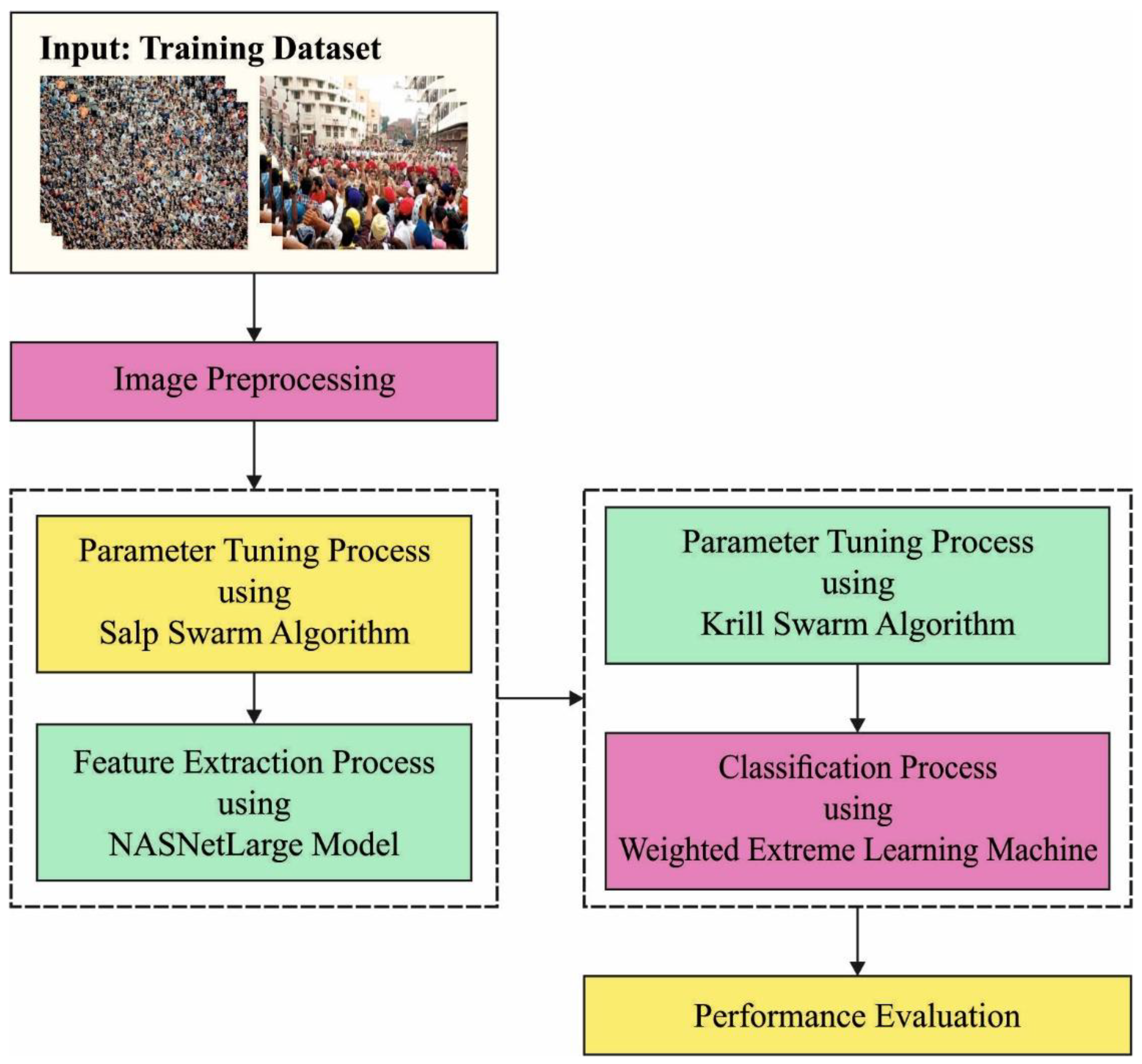
In this study, a new MDTL-ICDDC technique was established for effectual identification and classification of crowd density on a video surveillance system. The MDTL-ICDDC model initially presented an SSA with NASNetLarge model as a feature extraction model in which the hyperparameter tuning process is performed by the SSA. This was followed by the KSA-WELM model, which is employed for crowd-density and classification processes.
Figure 1 illustrates the block diagram of MDTL-ICDDC technique.
3.1. Feature Extraction Module
At the initial stage, the SSA with NASNetLarge model functions as a feature extraction model in which the hyperparameter tuning process is performed by the SSA. For determining the optimal convolution architecture for the dataset, a search algorithm can be used. Neural architecture search (NAS) is the most important search technique that the authors deployed in this network. Child network is shown to accomplish some accuracy on a validation set; in other words, it is used for convergence [
25]. The subsequent accuracy value is utilized to upgrade the controller that consecutively generates better architecture over time. The policy gradient takes place to update the controller weight.
A new searching space was designed, which permits the better architecture found on the CIFAR-10 dataset (available at
http://www.cs.toronto.edu/~kriz/cifar.html, accessed on 12 Febuary 2022) that generalized for large, high-resolution image datasets from the range of computation environments. To adapt input of depth of filtering and spatial dimension, this cell is sequentially stacked. In this technique, the convolution net overall architecture is predefined manually. They are composed of convolution cells that possess a similar shape as the original but are weighted in a different way. Two kinds of convolution cells have been taking place for rapidly developing scalable architecture for images of any size: (1) convolution cells return a feature map with a 2-fold reduction in width and height, and (2) convolution cells produce a feature map with the similar dimension.
Figure 2 depicts the framework of NasNetLarge.
These two kinds of convolution cells are represented as Normal Cell and Reduction Cell, correspondingly. The primary process used for the cell’s input gives a two-step stride to minimalize the cell’s width and height. The convolution cells support striding because they consider each operation. The Normal as well as Reduction Cells architecture that the controller RNN search for dissimilar to convolution net. The searching region is utilized for searching each cell shape. There are 2 hidden states (HS), namely h (i) and h (i −1), presented for every cell in the searching space. Initially, the HS is the outcome of 2 cells in the prior 2 lower layers or input image, correspondingly. The controller RNN make recursive prediction on the remaining convolution cells on the basis of 2 primary HSs. The controller prediction for all the cells is ordered into B blocks, with every block comprising five prediction steps implemented by five discrete SoftMax classifications representing different selections of block elements.
Step 1. Choose an HS from h (i), h (i −1), or the set of formerly generate HS.
Step 2. In the similar option as in Step1, choose the next HS.
Step 3. In Step 1, select the HS that the authors need to employ.
Step 4. After, choose an HS in Step2, choose an operation to employ.
Step 5. Define how the output from Steps 3 & 4 would be integrated to make a novel HS. It can be helpful to apply the recently generated HS as an input for the subsequent block.
For the optimal hyperparameter tuning process, the SSA is utilized. It was initially established as a swarm intelligence process [
26]; it can be stimulated by the foraging performance of the salp swarm that forms a chain. Similar to other algorithms, it finds an optimum solution via the cooperation and division of salps. The population is divided into the following categories: the leader and followers. Initially, the leaders lead the direction of the population, and next the follower follows them; consequently, the population forms a chain. The population
includes
agents are established as a matrix using D columns and N rows. The target population from the searching region is a food source represented as
.
whereas population size denotes
,
indicates dimension. The leader’s location is rehabilitated.
Now
and
mean the
parameter of the leader location and food source, respectively.
signifies a control variable adoptively decreased through the iteration and calculated. The role of exploration and exploitation is to determine SSA.
and
are created within
.
and
indicates the
variable of upper and lower limits, respectively.
Here,
and
denote the existing and maximal iterations, respectively. The follower location is rehabilitated as [
27].
where
and
indicates the
parameter in the position of
-
follower.
3.2. Crowd Density Classification Module
Once the feature vectors are created, the next stage is to classify the crowd density with the WELM model. WELM is an enhanced version of ELM that manages imbalanced class distribution data [
28]. The WELM approach presented the weighted matrix
similar to how the original ELM model works to balance the data distribution that weakens the majority class and strengthens the minority class. The
represents a matrix of misclassification values according to class distribution. The
in (5) signifies diagonal matrixes with
dimensional in which
indicates the overall dataset, and
denotes the overall amount of samples that belongings to class
.
The WELM is based on the standardized ELM that minimizes the error vector
, as well as minimizes the output weight norm
to have improved generalization outcomes. In the following, the mathematical expression of the minimization problem is given.
The solution of
is obtained from (6) on the basis of KKT condition into (7) if
is smaller and (8) if
is larger.
For multi-class classification with
class, all the labels are mapped into a vector of [−l, 1] through length of
; for example, a dataset that is categorized into the 2nd classes from three classes are
. The output
in multi-class classification is a vector
and the class label is evaluated by the following equation.
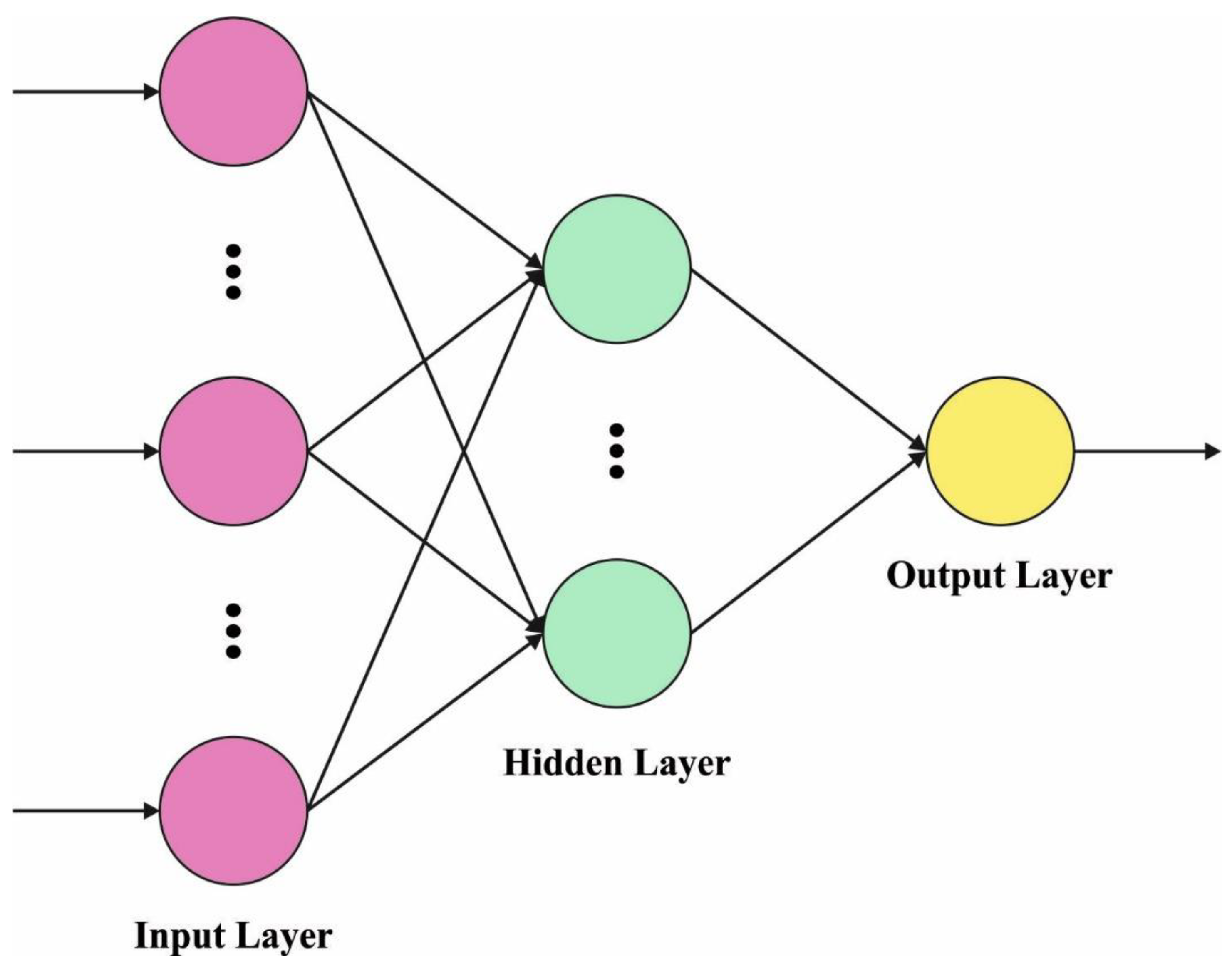
Figure 3 showcases the framework of WELM.
3.3. Parameter Tuning Process
For the optimal adjustment of the WELM parameters, the KSA is utilized in this study. The krill swarm algorithm (KSA) [
29] is a commonly used intelligent optimization technique, due to its benefits of strong search diversity, few adjusted parameters, and simple operation. The KSA approach originated from mutual communication and krill foraging. In the presented approach, the location of every individual krill represents a potential solution. The location of each krill is commonly specified in the following:
Individual swimming due to population migration:
From the equation, the maximum induction speed can be represented as , and taken as 0.01 and refers to the inertia weight of motion-induced range from [0, 1]. represents prior movement, whereas and indicate the target and the existing positions, respectively.
- 2.
Now, the individual direction of foraging for krill was denoted as . indicates the attractive direction of food, and indicates the direction of individual krill with the optimal fitness value. represents the foraging speed that takes as 0.02 and represents the inertia weight that ranges from [0, 1]. signifies the location change due to the preceding foraging motion of the - individual krill; denotes the location change due to the existing foraging motion of the individual - krill.
- 3.
Random diffusion of individual krill:
In Equation (14), indicates the maximal disturbance (diffusion) velocity, and denotes an arbitrary direction vector that ranges from signifies the location change due to arbitrary diffusion of - individual krill.
The swimming direction of each krill can be defined by the fusion of abovementioned factors that change in the direction with minimum fitness value. The foraging and induced motions have local and global searching functions. After the process is iteratively updated, two measures are simultaneously implemented, which make stable and powerful optimization algorithms.
The location vector from
to
is formulated by:
Here,
indicates the factor for the step size.
Now, indicates the overall amount of parameters, whereas and denote the upper as well as lower bounds of the - parameter.
The KSA system grows a fitness function (FF) for attaining higher classifier performance. It resolves the positive integer for denoting the best efficiency of candidate results. In this work, the minimization of the classification error rate is measured FF, as shown in Equation (17).
4. Results and Discussion
In this section, the experimental validation of the MDTL-ICDDC model is tested with a dataset comprising 1000 images under four class labels. The MDTL-ICDDC model is simulated using Python 3.6.5 tool on a PC i5-8600k, GeForce 1050Ti 4 GB, 16 GB RAM, 250GB SSD, and 1 TB HDD. The parameter settings are given as follows: learning rate: 0.01, dropout: 0.5, batch size: 5, epoch count: 50, and activation: ReLU. Few sample images are demonstrated in
Figure 4. The details related to the dataset are given in
Table 1.
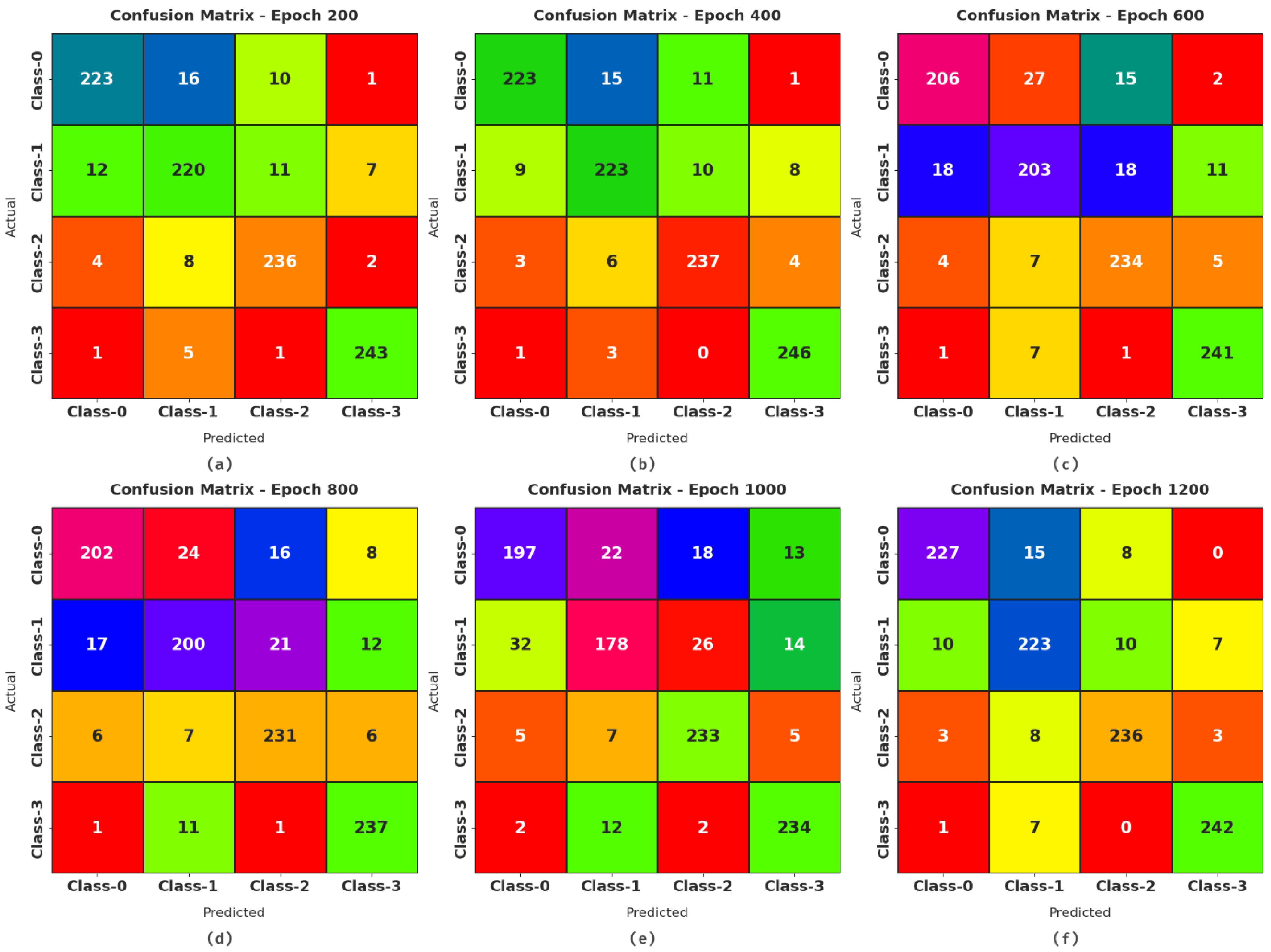
Figure 5 demonstrates a set of confusion matrices formed by the MDTL-ICDDC model on distinct epoch counts. On epoch 200, the MDTL-ICDDC model has recognized 223, 220, 236, and 243 images under classes 0–3 respectively. Moreover, on epoch 600, the MDTL-ICDDC technique has recognized 206, 203, 234, and 241 images under classes 0–3 respectively. At the same time, on epoch 1000, the MDTL-ICDDC approach has recognized 197, 178, 233, and 234 images under classes 0–3 respectively. In line with, epoch 1200, the MDTL-ICDDC system has recognized 227, 178, 236, and 242 images under classes 0–3 respectively.
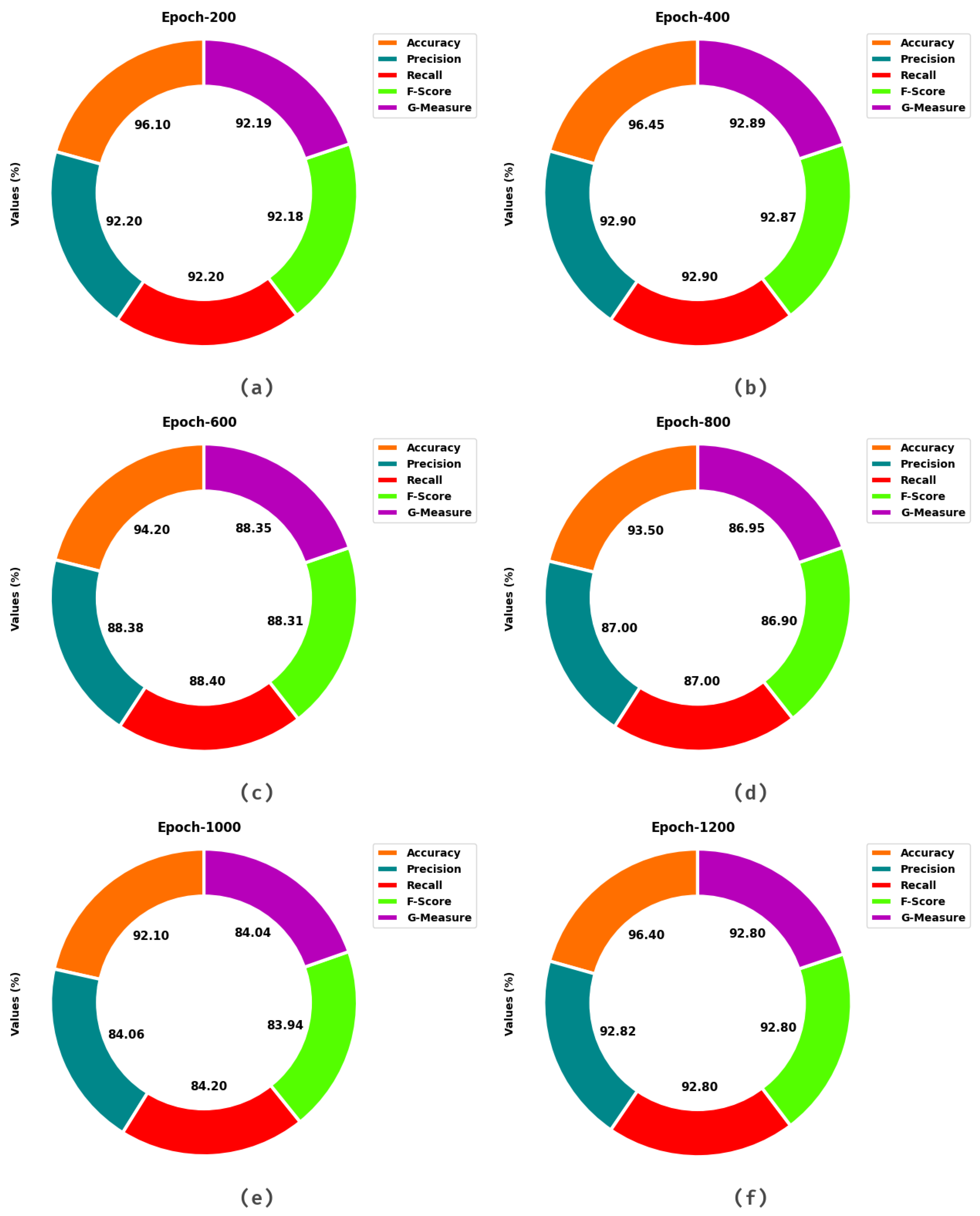
Table 2 and
Figure 6 offer a detailed crowd density classification outcome of the MDTL-ICDDC model under distinct epochs and classes. The results indicated that the MDTL-ICDDC model has gained effectual outcomes under all classes and epochs. For instance, with 200 epochs, the MDTL-ICDDC model has provided average
,
,
,
, and
of 96.10%, 92.20%, 92.20%, 92.18%, and 92.19% respectively. Likewise, with 600 epochs, the MDTL-ICDDC technique has obtainable average
,
,
,
, and
of 94.20%, 88.38%, 88.40%, 88.31%, and 88.35% respectively. Similarly, with 1000 epochs, the MDTL-ICDDC system has provided average
,
,
,
, and
of 92.10%, 84.06%, 84.20%, 83.94%, and 84.04% respectively. Eventually, with 1200 epochs, the MDTL-ICDDC methodology has offered average
,
,
,
, and
of 96.40%, 92.82%, 92.80%, 92.80%, and 92.80% respectively.
The training accuracy (TA) and validation accuracy (VA) attained by the MDTL-ICDDC method on test dataset are demonstrated in
Figure 7. The experimental outcome implied that the MDTL-ICDDC model has gained maximal values of TA and VA. Specfically, the VA seemed superior to the TA.
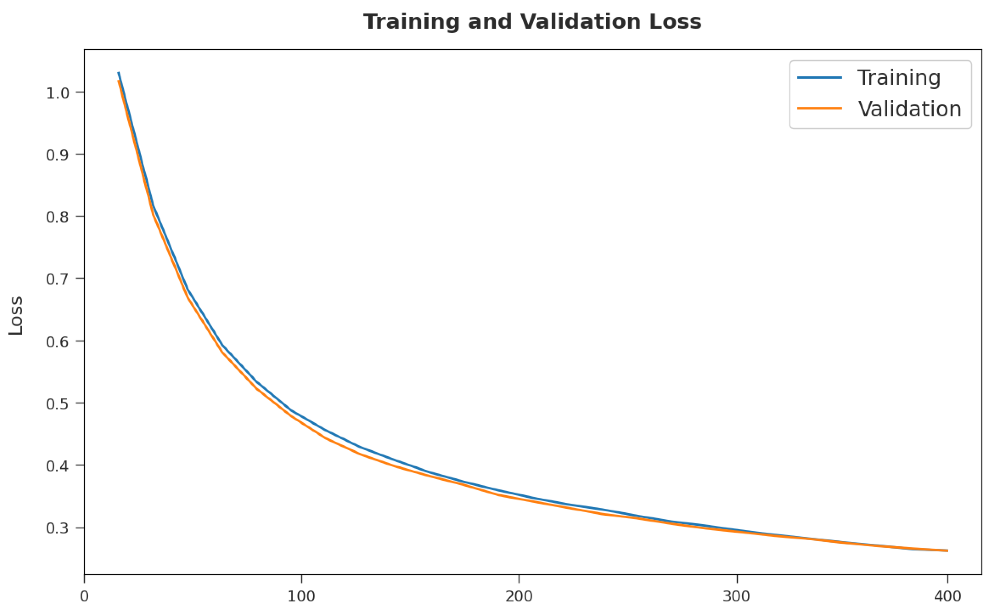
The training loss (TL) and validation loss (VL) achieved by the MDTL-ICDDC model on test dataset are displayed in
Figure 8. The experimental outcome exposed that the MDTL-ICDDC technique has been able least values of TL and VL. Specifically, the VL seemed lower than the TL.
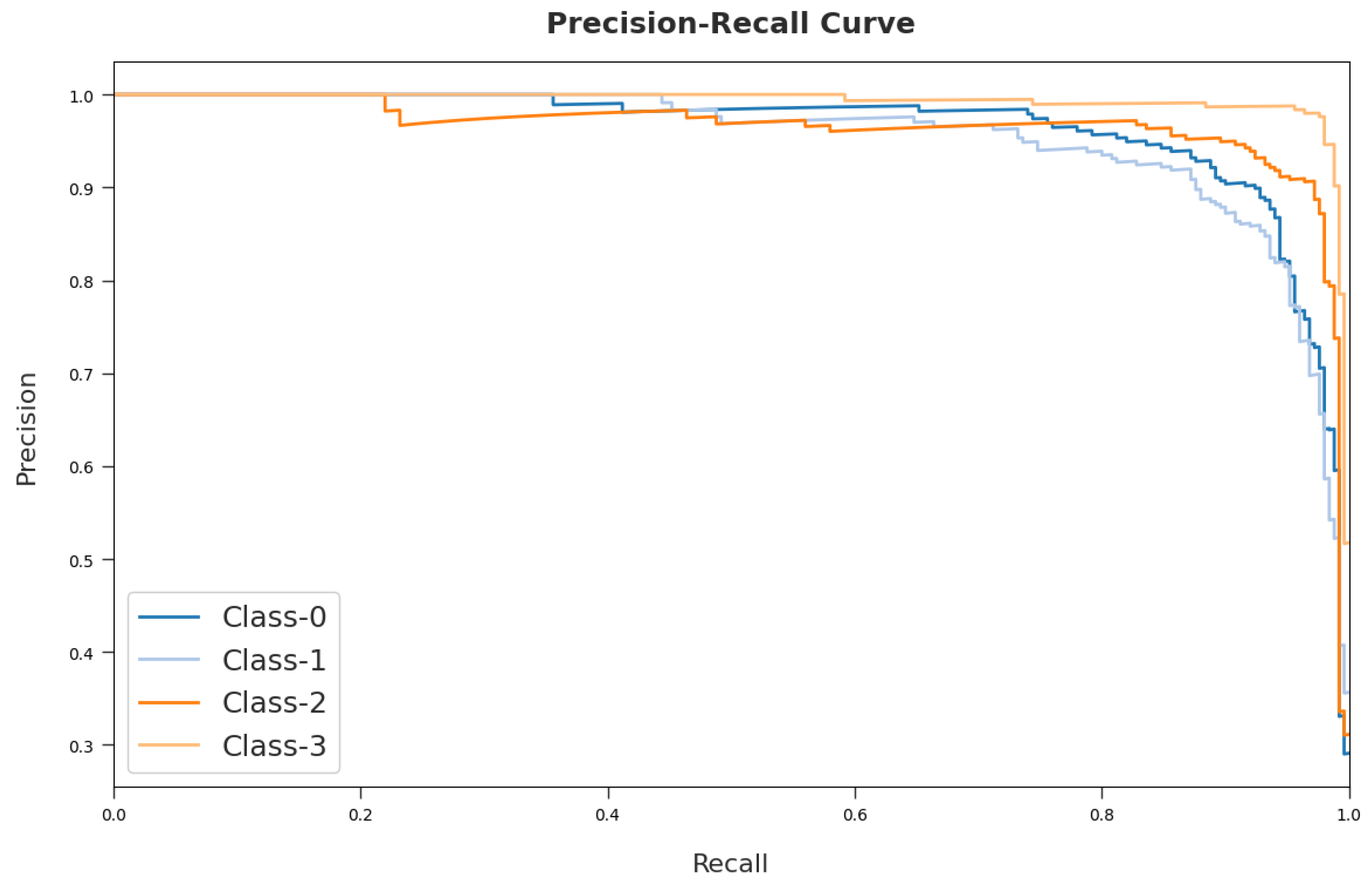
A brief precision-recall examination of the MDTL-ICDDC method on test dataset is portrayed in
Figure 9. An observation of the figure shows that the MDTL-ICDDC system has been able to achieve maximal precision-recall performance under all classes.
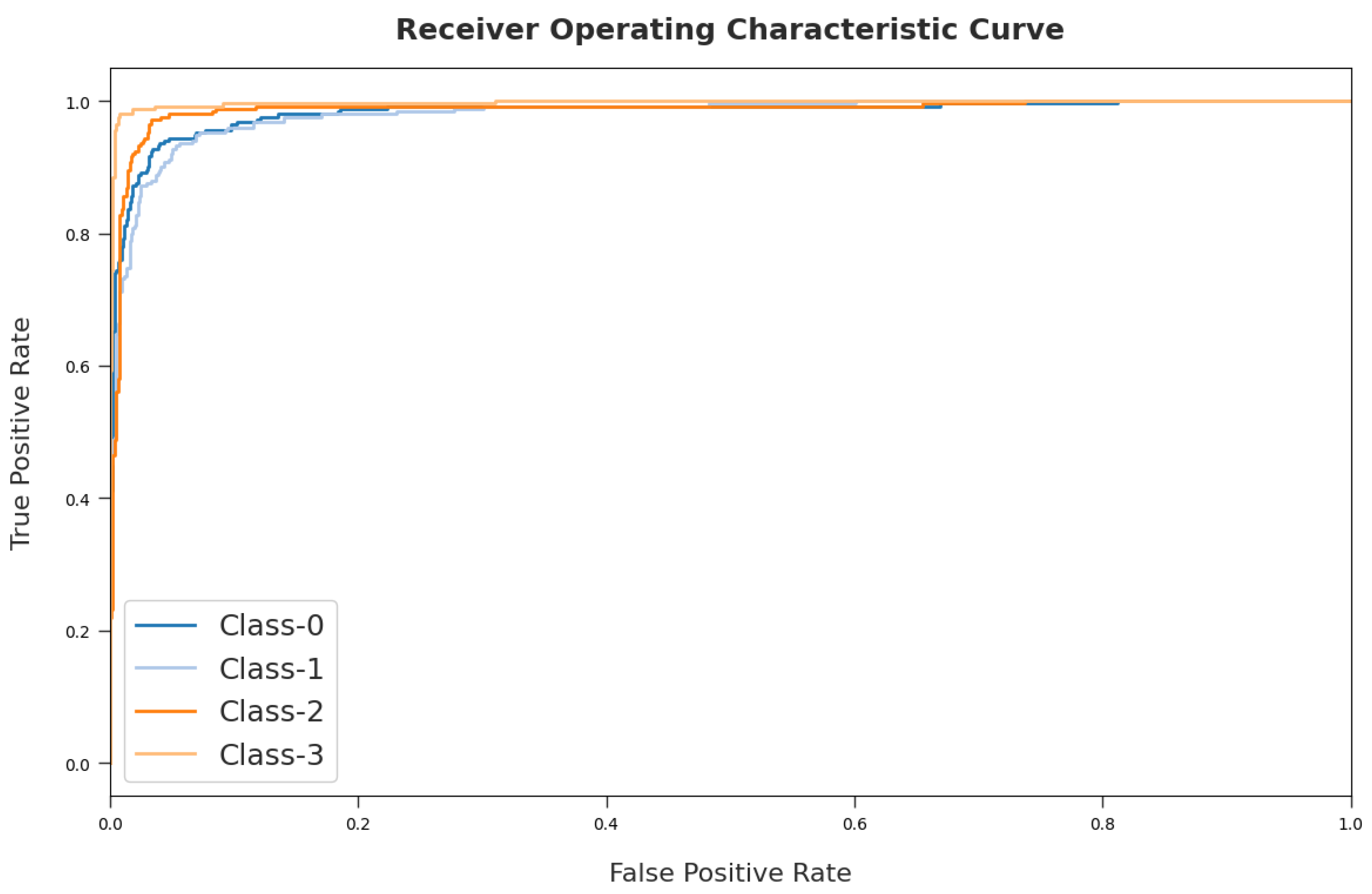
A detailed ROC investigation of the MDTL-ICDDC approach on test dataset is depicted in
Figure 10. The results indicated that the MDTL-ICDDC model has exhibited its ability in categorizing four different classes 0–3 on the test dataset.
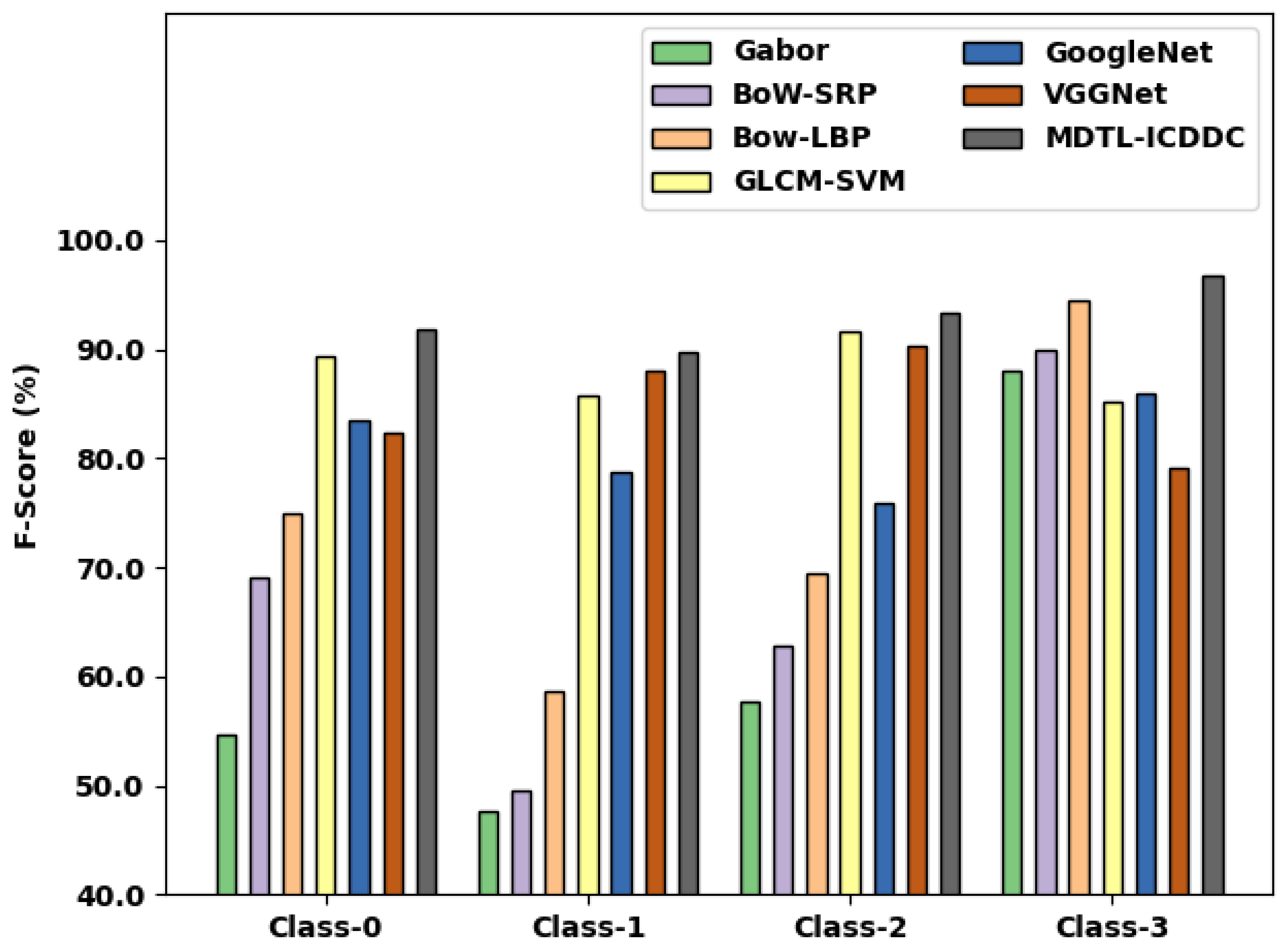
Table 3 and
Figure 11 inspect a comparative
inspection of the MDTL-ICDDC model with other models under distinct classes [
30,
31]. The experimental results indicated that the Gabor and BoW-SRP models have shown lower classification results with least average
of 61.83% and 68.33% respectively. Likewise, the BoW-LBP and GLCM-SVM models have accomplished slightly improved average
values of 74.68% and 75.47% respectively. At the same time, the GoogleNet and VGGNet techniques have resulted in reasonable average
values of 82.98% and 86.14% respectively. However, the MDTL-ICDDC model has gained maximum average
of 92.90%.
Table 4 and
Figure 12 demonstrate a comparative
analysis of the MDTL-ICDDC approach with other models under distinct classes. The experimental results indicated that the Gabor and BoW-SRP models have shown lower classification results with least average
of 62.30% and 67.85% respectively. Moreover, the BoW-LBP and GLCM-SVM models have accomplished somewhat enhanced average
values of 74.15% and 73.52% correspondingly. Simultaneously, the GoogleNet and VGGNet techniques have resulted in reasonable average
values of 85.26% and 82.78% respectively. But, the MDTL-ICDDC model has gained maximal average
of 92.90%.
Table 5 and
Figure 13 depict a comparative
examination of the MDTL-ICDDC model with other algorithms under distinct classes. The experimental results indicated that the Gabor and BoW-SRP approaches have shown lower classification results with least average
of 71.83% and 80.40% respectively. Alongside these results, the BoW-LBP and GLCM-SVM methods have accomplished slightly improved average
values of 84.04% and 79.78% respectively. These results are followed by the GoogleNet and VGGNet approaches, which have resulted in reasonable average
values of 84.40 and 84.75% respectively. At last, the MDTL-ICDDC method has gained higher average
of 96.45%.
Table 6 and
Figure 14 illustrate a comparative
inspection of the MDTL-ICDDC algorithm with other techniques under distinct classes. The experimental results indicated that the Gabor and BoW-SRP models have exposed lesser classification results with minimal average
of 61.98% and 67.88% respectively. In addition, the BoW-LBP and GLCM-SVM models have accomplished somewhat higher average
values of 74.35% and 87.99% respectively.
Moreover, the GoogleNet and VGGNet approaches have resulted in reasonable average values of 81% and 84.95% respectively. Finally, the MDTL-ICDDC model has gained superior average of 92.87%. These results and discussion pointed out that the MDTL-ICDDC model has proficiently detected and classified the crowd density in enabled video surveillance systems.


 ,
, 


