
Study and Design of a Machine Learning-Enabled Laser-Based Sensor for Pure and Sea Water Determination Using COMSOL Multiphysics


Abstract
:1. Introduction
2. Literature Review
2.1. Direct Measurement Techniques
2.2. Indirect Measurement Techniques
2.2.1. Acoustic Method
2.2.2. Density Method
2.2.3. Conductivity Method
2.2.4. Optics Method
2.3. Our Proposed Solution
3. Concept and Methodology
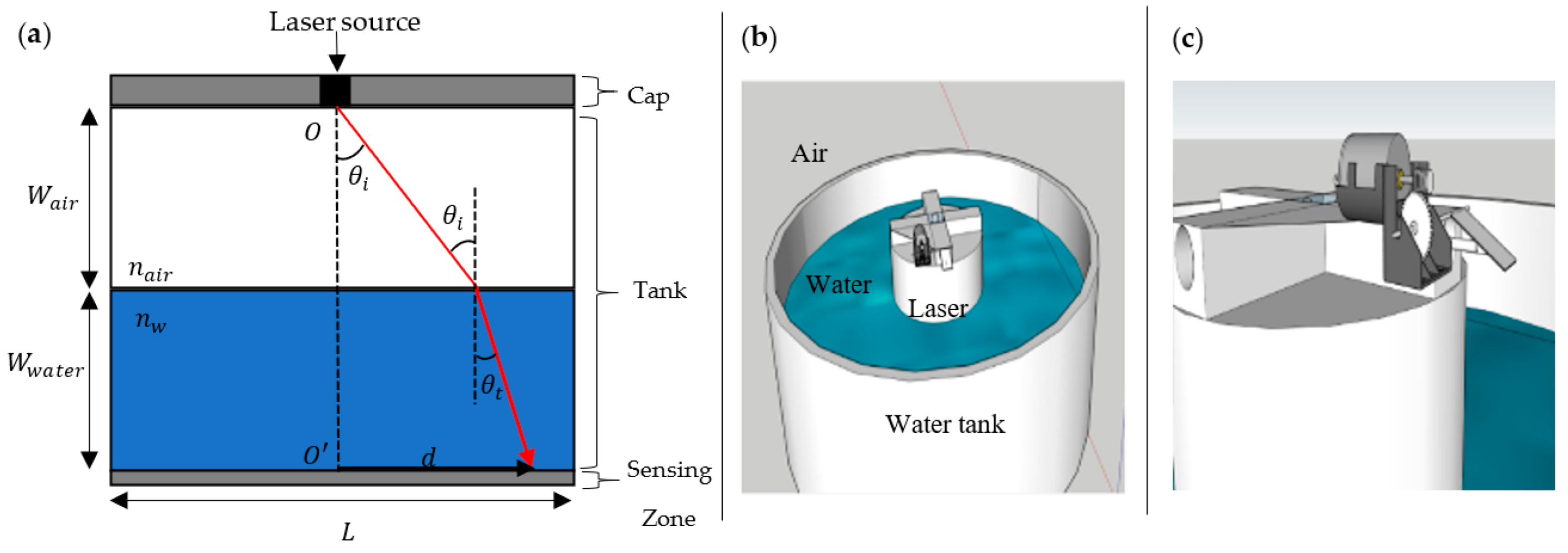
3.1. Sensor Concept and Design
3.2. COMSOL Multiphysics Simulation
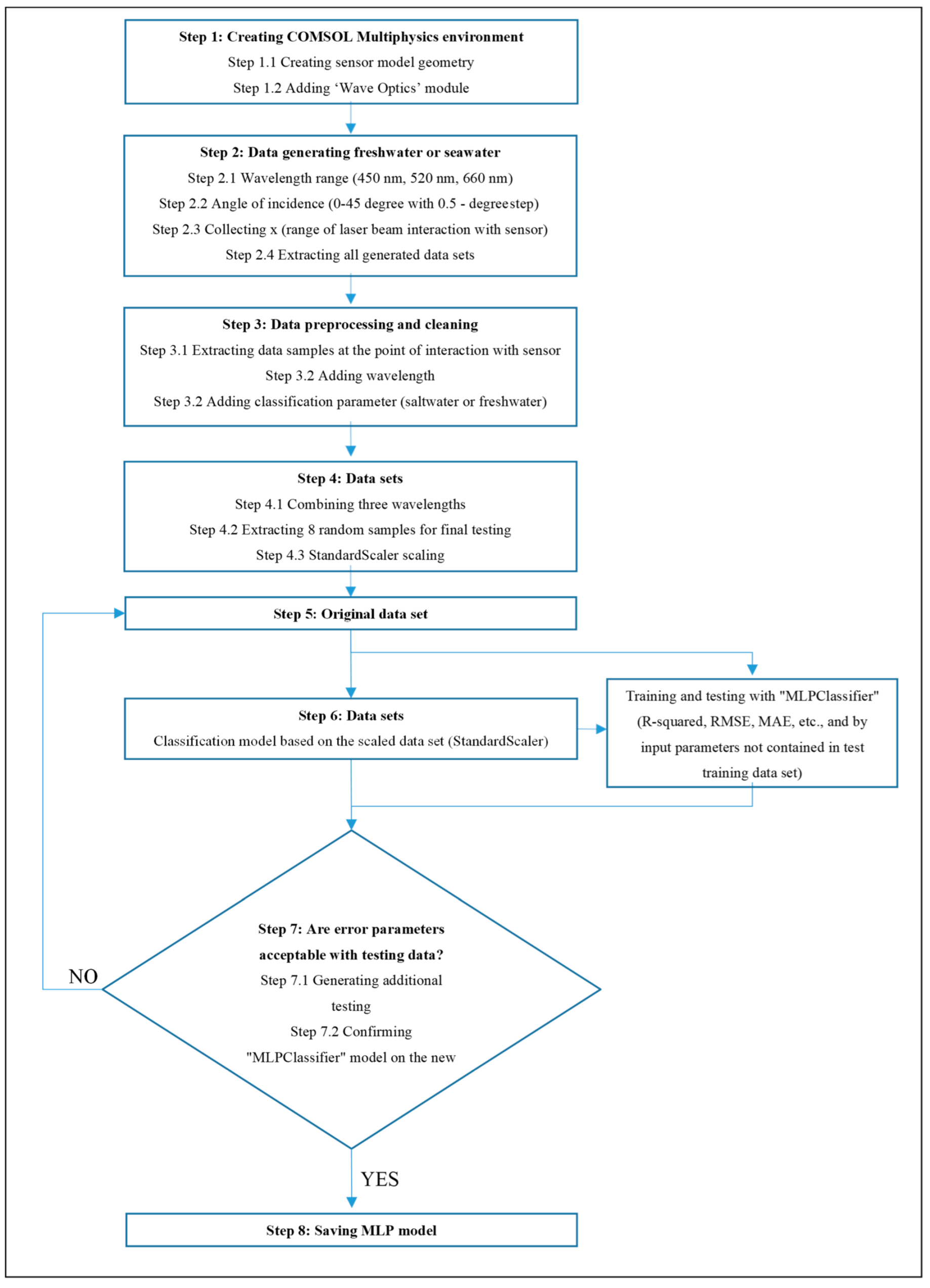
3.3. Machine Learning and Data
- (1)
- Incident angle from 0 to 45° with 0.5° step;
- (2)
- Air-water concentration (cm) with six different configurations (15/5, 14/6, 13/7, 12/8, 11/9, 10/10);
- (3)
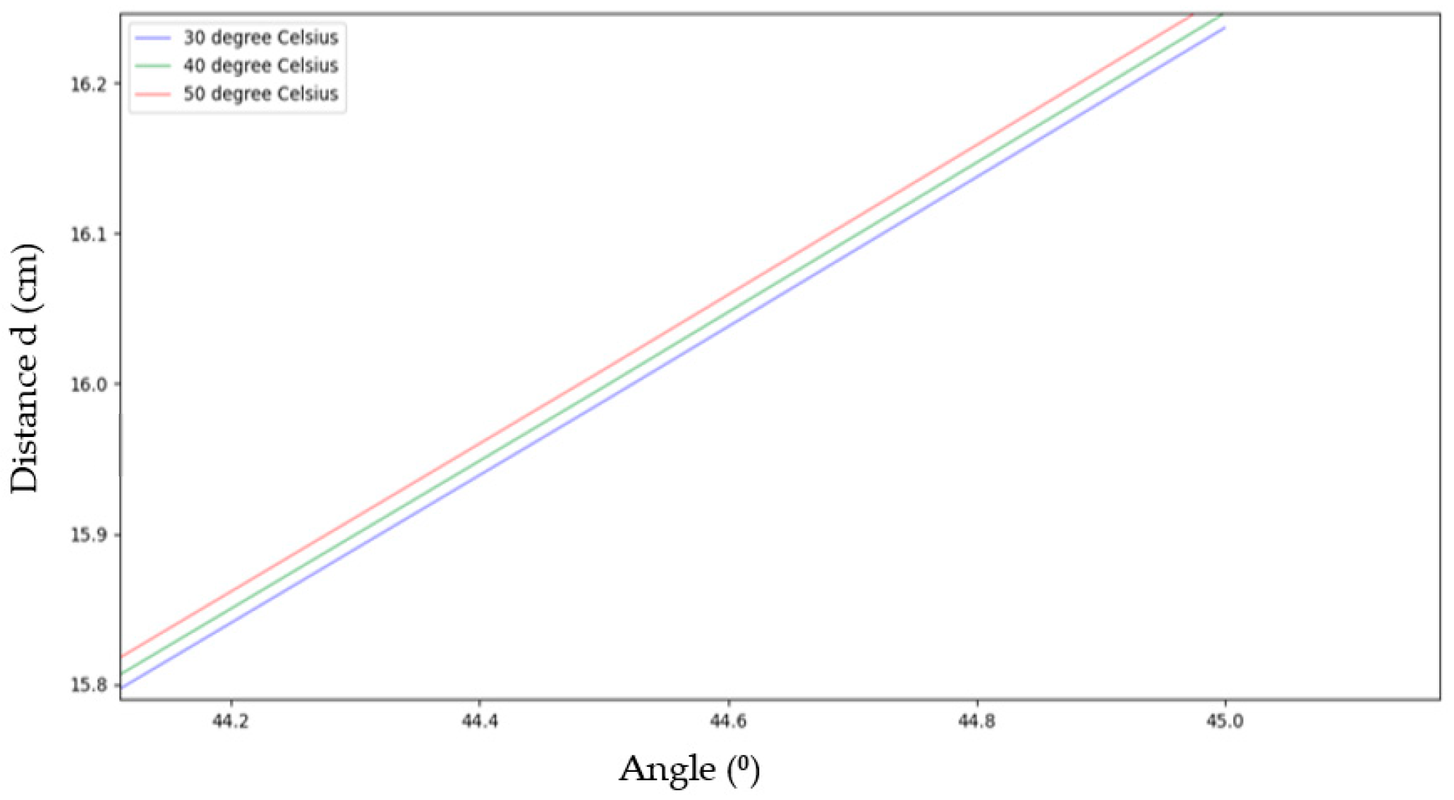
- Temperature T with three different configurations (30, 40, and 50 °C, respectively);
- (4)
- Wavelength λ with three different configurations (450, 520, and 660 nm, respectively).
4. Results and Discussion
5. Conclusions
Author Contributions
Funding
Conflicts of Interest
References
- Alberto, N.; Tavares, C.; Domingues, M.F.; Correia, S.F.H.; Marques, C.; Antunes, P.; Pinto, J.L.; Ferreira, R.A.S.; André, P.S. Relative humidity sensing using micro-cavities produced by the catastrophic fuse effect. Opt. Quant. Electron. 2016, 48, 216. [Google Scholar] [CrossRef]
- Marques, C.A.; Bilro, L.B.; Alberto, N.J.; Webb, D.J.; Nogueira, R.N. Narrow bandwidth Bragg gratings imprinted in polymer optical fibers for different spectral windows. Opt. Commun. 2013, 307, 57–61. [Google Scholar] [CrossRef]
- Guo, Y.; Li, J.; Wang, X.; Zhang, S.; Liu, Y.; Wang, J.; Wang, S.; Meng, X.; Hao, R.; Li, S. Highly sensitive sensor based on D-shaped microstructure fiber with hollow core. Opt. Laser Technol. 2020, 123, 105922. [Google Scholar] [CrossRef]
- Yaroshenko, I.; Kirsanov, D.; Marjanovic, M.; Lieberzeit, P.A.; Korostynska, O.; Mason, A.; Frau, I.; Legin, A. Real-Time Water Quality Monitoring with Chemical Sensors. Sensors 2020, 20, 3432. [Google Scholar] [CrossRef] [PubMed]
- Meyer, A.M.; Klein, C.; Fünfrocken, E.; Kautenburger, R.; Beck, H.P. Real-time monitoring of water quality to identify pollution pathways in small and middle scale rivers. Sci. Total Environ. 2018, 651, 2323–2333. [Google Scholar] [CrossRef] [PubMed]
- Capella, J.; Bonastre, A.; Ors, R.; Peris, M. A Wireless Sensor Network approach for distributed in-line chemical analysis of water. Talanta 2010, 80, 1789–1798. [Google Scholar] [CrossRef]
- Qian, Y.; Zhao, Y.; Wu, Q.-L.; Yang, Y. Review of salinity measurement technology based on optical fiber sensor. Sens. Actuators B Chem. 2018, 260, 86–105. [Google Scholar] [CrossRef]
- Wang, Y.; Guo, J.; Yang, Z.; Dou, Y.; Chang, X.; Sun, R.; Zuo, G.; Yang, W.; Liang, C.; Hao, Y.; et al. Computer Prediction of Seawater Sensor Parameters in the Central Arctic Region Based on Hybrid Machine Learning Algorithms. IEEE Access 2020, 8, 213783–213798. [Google Scholar] [CrossRef]
- Cipollini, P.; Corsini, G.; Diani, M.; Grasso, R. Retrieval of sea water optically active parameters from hyperspectral data by means of generalized radial basis function neural networks. IEEE Trans. Geosci. Remote Sens. 2001, 39, 1508–1524. [Google Scholar] [CrossRef]
- Agha, M.; Ennen, J.R.; Bower, D.; Nowakowski, A.J.; Sweat, S.C.; Todd, B. Salinity tolerances and use of saline environments by freshwater turtles: Implications of sea level rise. Biol. Rev. 2018, 93, 1634–1648. [Google Scholar] [CrossRef]
- Huber, C.; Klimant, I.; Krause, C.; Werner, T.; Mayr, T.; Wolfbeis, O.S. Optical sensor for seawater salinity. Anal. Bioanal. Chem. 2000, 368, 196–202. [Google Scholar] [CrossRef] [PubMed]
- Huber, C.; Klimant, I.; Krause, C.; Wolfbeis, O.S. Dual Lifetime Referencing as Applied to a Chloride Optical Sensor. Anal. Chem. 2001, 73, 2097–2103. [Google Scholar] [CrossRef] [PubMed]
- An, S.; Ko, D.; Noh, J.; Lee, C.; Seo, D.; Lee, M.; Chang, J. ITO Nanoparticle Chemiresistive Sensor for Detecting Liquid Chemicals Diluted in Brine. Trans. Electr. Electron. Mater. 2022, 23, 107–112. [Google Scholar] [CrossRef]
- Grekov, A.N.; Grekov, N.A.; Sychov, E.N. New Equations for Sea Water Density Calculation Based on Measurements of the Sound Speed. Mekhatronika Avtom. Upr. 2019, 20, 143–151. [Google Scholar] [CrossRef] [Green Version]
- You, B.; Yue, Y.; Sun, M.; Li, J.; Jia, D. Design of a Real-Time Salinity Detection System for Water Injection Wells Based on Fuzzy Control. Sensors 2021, 21, 3086. [Google Scholar] [CrossRef]
- Schmidt, H.; Wolf, H.; Hassel, E. A method to measure the density of seawater accurately to the level of 10−6. Metrologia 2016, 53, 770–786. [Google Scholar] [CrossRef]
- Woosley, R.J.; Huang, F.; Millero, F.J. Estimating absolute salinity (SA) in the world’s oceans using density and composition. Deep-Sea Res. Part I 2014, 93, 14–20. [Google Scholar] [CrossRef]
- Dong, T.; Barbosa, C. Capacitance Variation Induced by Microfluidic Two-Phase Flow across Insulated Interdigital Electrodes in Lab-On-Chip Devices. Sensors 2015, 15, 2694–2708. [Google Scholar] [CrossRef] [Green Version]
- Wu, H.; Tan, C.; Dong, X.; Dong, F. Design of a Conductance and Capacitance Combination Sensor for water holdup measurement in oil–water two-phase flow. Flow Meas. Instrum. 2015, 46, 218–229. [Google Scholar] [CrossRef]
- Zhai, L.S.; Jin, N.D.; Gao, Z.K.; Wang, Z.Y. Liquid holdup measurement with double helix capacitance sensor in horizontal oil-water two-phase flow pipes. Chin. J. Chem. Eng. 2015, 23, 268–275. [Google Scholar] [CrossRef]
- Ramos, P.M.; Pereira, J.M.D.; Ramos, H.M.G.; Ribeiro, A.L. A four terminal water quality monitoring conductivity sensor. IEEE Trans. Instrum. Meas. 2008, 57, 577–583. [Google Scholar] [CrossRef]
- Huang, X.; Pascal, R.; Chamberlain, K.; Banks, C.; Mowlem, M.; Morgan, H. A miniature, high precision conductivity and temperature sensor system for ocean monitoring. IEEE Sens. J. 2011, 11, 3246–3252. [Google Scholar] [CrossRef]
- Intergovernmental Oceanographic Commission. The International Thermodynamic Equation of Seawater—2010: Calculation and Use of Thermodynamic Properties; IOC: Paris, France, 2010; Available online: http://www.go-ship.org/HydroMan.html (accessed on 17 May 2022).
- CTD Profilers. Available online: https://www.seabird.com/products/profilers.htm (accessed on 17 May 2022).
- McDougall, T.J.; Jackett, D.R.; Millero, F.J.; Pawlowicz, R.; Barker, P.M. A global algorithm for estimating Absolute Salinity. Ocean Sci. 2012, 8, 1123–1134. [Google Scholar] [CrossRef] [Green Version]
- Xiao, A.; Huang, Y.; Zheng, J.; Chen, P.; Guan, B.-O. An Optical Microfiber Biosensor for CEACAM5 Detection in Serum: Sensitization by a Nanosphere Interface. ACS Appl. Mater. Interfaces 2020, 12, 1799–1805. [Google Scholar] [CrossRef] [PubMed]
- Wang, Q.; Wang, X.-Z.; Song, H.; Zhao, W.-M.; Jing, J.-Y. A dual channel self-compensation optical fiber biosensor based on coupling of surface plasmon polariton. Opt. Laser Technol. 2020, 124, 106002. [Google Scholar] [CrossRef]
- Liu, Q.; Ma, Z.; Wu, Q.; Wang, W. The biochemical sensor based on liquid-core photonic crystal fiber filled with gold, silver and aluminum. Opt. Laser Technol. 2020, 130, 106363. [Google Scholar] [CrossRef]
- Rifat, A.A.; Mahdiraji, G.A.; Sua, Y.M.; Ahmed, R.; Shee, Y.G.; Adikan, F.R.M. Highly sensitive multi-core flat fiber surface plasmon resonance refractive index sensor. Opt. Express 2016, 24, 2485–2495. [Google Scholar] [CrossRef]
- Lin, Q.; Hu, Y.; Yan, F.; Hu, S.; Chen, Y.; Liu, G.; Chen, L.; Xiao, Y.; Chen, Y.; Luo, Y.; et al. Half-side gold-coated hetero-core fiber for highly sensitive measurement of a vector magnetic field. Opt. Lett. 2020, 45, 4746. [Google Scholar] [CrossRef]
- Momtaj, M.; Mou, J.R.; Kamrunnahar, Q.M.; Islam, A. Open-channel-based dual-core D-shaped photonic crystal fiber plasmonic biosensor. Appl. Opt. 2020, 59, 8856–8865. [Google Scholar] [CrossRef]
- Luan, N.; Yao, J. Refractive Index and Temperature Sensing Based on Surface Plasmon Resonance and Directional Resonance Coupling in a PCF. IEEE Photon J. 2017, 9, 6801307. [Google Scholar] [CrossRef]
- Wang, H.; Dai, W.; Cai, X.; Xiang, Z.; Fu, H.; Ieee, M. Half-side PDMS-coated dual-parameter PCF sensor for simultaneous measurement of seawater salinity and temperature. Opt. Fiber Technol. 2021, 65, 102608. [Google Scholar] [CrossRef]
- Zhong, S.; Fan, Y.; Xue, Y.; Wang, Y.; Liu, R. Combined LIBS and Raman spectroscopy: A newapproach for salinity detection in the field ofseawater investigation. Appl. Opt. 2022, 61, 1718–1725. [Google Scholar] [CrossRef]
- Hu, C.; Voss, K.J. In situ measurements of Raman scattering in clear ocean water. Appl. Opt. 1997, 36, 6962–6967. [Google Scholar] [CrossRef] [PubMed] [Green Version]
- Cong, J.; Zhang, X.; Chen, K.; Xu, J. Fiber optic Bragg grating sensor based on hydrogels for measuring salinity. Sens. Actuators B Chem. 2002, 87, 487–490. [Google Scholar] [CrossRef]
- Liu, X.; Zhang, X.; Cong, J.; Xu, J.; Chen, K. Demonstration of etched cladding fiber Bragg grating-based sensors with hydrogel coating. Sens. Actuators B Chem. 2003, 96, 468–472. [Google Scholar] [CrossRef]
- Gentleman, D.J.; Booksh, K.S. Determining salinity using a multimode fiber optic surface plasmon resonance dip-probe. Talanta 2006, 68, 504–515. [Google Scholar] [CrossRef]
- Lee, K.; Hassan, A.; Lee, C.H.; Bae, J. Microstrip Patch Sensor for Salinity Determination. Sensors 2017, 17, 294. [Google Scholar] [CrossRef] [Green Version]
- Zhang, X.; Peng, W. Temperature-independent fiber salinity sensor based on Fabry-Perot interference. Opt. Express 2015, 23, 10353. [Google Scholar] [CrossRef]
- Wu, C.; Sun, L.; Li, J.; Guan, B. Highly sensitive evanescent-wave water salinity sensor realized with rectangular optical microfiber Sagnac interferometer. In Proceedings of the 23rd International Conference on Optical Fiber Sensors, Santander, Spain, 2–6 June 2014; Volume 9157. [Google Scholar] [CrossRef]
- Jaddoa, M.; Jasim, A.; Razak, M.; Harun, S.; Ahmad, H. Highly responsive NaCl detector based on inline microfiber Mach–Zehnder interferometer. Sens. Actuators A 2016, 237, 56–61. [Google Scholar] [CrossRef]
- Li, L.; Xia, L.; Wuang, Y.; Ran, Y.; Yang, C.; Liu, D. Novel NCF-FBG Interferometer for Simultaneous Measurement of Refractive Index and Temperature. IEEE Photon Technol. Lett. 2012, 24, 2268–2271. [Google Scholar] [CrossRef]
- Grosso, P.; Malardé, D.; Le Menn, M.; Wu, Z.; de Bougrenet de la Tocnaye, J.L. Refractometer resolution limits for measuring seawater refractive index. Opt. Eng. 2010, 49, 103603. [Google Scholar] [CrossRef]
- Malardé, D.; Wu, Z.Y.; Grosso, P.; de Bougrenet de la Tocnaye, J.L.; Le Menn, M. High-resolution and compact refractometer for salinity measurements. Meas. Sci. Technol. 2009, 20, 015204. [Google Scholar] [CrossRef]
- Aly, K.M.; Esmail, E. Refractive index of salt water: Effect of temperature. Opt. Mater. 1993, 2, 195–199. [Google Scholar] [CrossRef]
- Chen, J.; Guo, W.; Xia, M.; Li, W.; Yang, K. In situ measurement of seawater salinity with an optical refractometer based on total internal reflection method. Opt. Express 2018, 26, 25510–25523. [Google Scholar] [CrossRef] [PubMed]
- Díaz-Herrera, N.; Esteban, O.; Navarrete, M.C.; Le Haitre, M.; González-Cano, A. In situ salinity measurements in seawater with a fibre-optic probe. Meas. Sci. Technol. 2006, 17, 2227–2232. [Google Scholar] [CrossRef] [Green Version]
- Qiu, Z. A simple optical model to estimate suspended particulate matter in Yellow River Estuary. Opt. Express 2013, 21, 27891–27904. [Google Scholar] [CrossRef]
- Röttgers, R.; McKee, D.; Utschig, C. Temperature and salinity correction coefficients for light absorption by water in the visible to infrared spectral region. Opt. Express 2014, 22, 25093–25108. [Google Scholar] [CrossRef] [Green Version]
- Artlett, C.P.; Pask, H. New approach to remote sensing of temperature and salinity in natural water samples. Opt. Express 2017, 25, 2840–2851. [Google Scholar] [CrossRef]
- Minato, H.; Kakui, Y.; Nishimoto, A.; Nanjo, M. Remote refractive index difference meter for salinity sensor. IEEE Trans. Instrum. Meas. 1989, 38, 608–612. [Google Scholar] [CrossRef]
- Millard, R.; Seaver, G. An index of refraction algorithm for seawater over temperature, pressure, salinity, density, and wavelength. Deep Sea Res. Part A. Oceanogr. Res. Pap. 1990, 37, 1909–1926. [Google Scholar] [CrossRef]
- Quan, X.; Fry, E.S. Empirical equation for the index of refraction of seawater. Appl. Opt. 1995, 34, 3477–3480. [Google Scholar] [CrossRef] [PubMed]
- Mcneil, G.T. Metrical Fundamentals of Underwater Lens System. Opt. Eng. 1977, 16, 1079–1095. [Google Scholar] [CrossRef]
- Index of Refraction of Seawater and Freshwater as a Function of Wavelength and Temperature, Parrish Research Group, Oregon State University. Available online: http://research.engr.oregonstate.edu/parrish/index-refraction-seawater-and-freshwater-function-wavelength-and-temperature (accessed on 17 May 2022).
- Austin, R.W.; Halikas, G. The Index of Refraction of Seawater; SIO Ref. No. 76-1; Scripps Institution of Oceanography: San Diego, CA, USA, 1976. [Google Scholar]
- Mobley, C.D. The optical properties of water. In Handbook of Optics, 3rd ed.; Bass, M., Ed.; McGraw-Hill: New York, NY, USA, 2010; Volume 4, pp. 1.3–1.53. [Google Scholar]
- Weigend, A.; Rumelhart, D.; Huberman, B. Generalization by weight-elimination with application to forecasting. In Advances in Neural Information Processing Systems; Morgan Kaufmann Publishers: Burlington, MA, USA, 1991; pp. 875–882. [Google Scholar]
- Zweiri, Y.H.; Seneviratne, L.D.; Althoefer, K. Stability analysis of a three-term backpropagation algorithm. Neural Netw. 2005, 18, 1341–1347. [Google Scholar] [CrossRef]
- Pedregosa, F.; Varoquaux, G.; Gramfort, A.; Michel, V.; Thirion, B.; Grisel, O.; Blondel, M.; Prettenhofer, P.; Weiss, R.; Dubourg, V.; et al. Scikit-learn: Machine Learning in Python. J. Mach. Learn. Res. 2011, 12, 2825–2830. [Google Scholar] [CrossRef]


| Reference | Method/Technique | Advantages | Disadvantages/Limitations |
|---|---|---|---|
| [10,11,12,13] | Chemicals (lucigenin, luminophores membranes…) |
|
|
| [14,15] | Acoustic/density |
|
|
| [18,19,20,21,22,23,24,25] | Conductivity |
|
|
| [29,32,33] | Surface Plasmon Resonance |
|
|
| [34,35] | Raman scattering |
|
|
| [40,41,42,43,44,45,46,47,48,49,50,51] | Interferometer/refractive index |
|
|
| [8,9] | Machine learning |
|
|
| Example | Distance d (cm) Using Equation (3) | Distance d (cm) Using COMSOL | Error |
|---|---|---|---|
| 1 | 3.29951 | 3.29950 | |
| 2 | 8.56587 | 8.56588 | |
| 3 | 16.63138 | 16.63126 | |
| 4 | 13.03546 | 13.03559 |
| INPUT | OUTPUT | ||||||||
|---|---|---|---|---|---|---|---|---|---|
| Configuration 1 | Configuration 2 | Configuration 3 | |||||||
| (°) | Air/water concentration (cm) | T (°C) | Distance d (cm) | λ (nm) | Distance d (cm) | λ (nm) | Distance d (cm) | λ (nm) | Water sample |
| 42.5 | 15/5 | 30 | 16.668650 | 450 | 16.67984 | 520 | 16.69381 | 660 | 0 |
| 8.5 | 14/6 | 30 | 2.7557548 | 450 | 2.757758 | 520 | 2.760128 | 660 | 1 |
| 14.5 | 13/7 | 50 | 4.6986000 | 450 | 4.702555 | 520 | 4.707375 | 660 | 0 |
| 18 | 14/6 | 50 | 5.9764883 | 450 | 5.980795 | 520 | 5.986045 | 660 | 0 |
| 23 | 10/10 | 40 | 7.2846954 | 450 | 7.294368 | 520 | 7.306362 | 660 | 1 |
| Coefficient of Determination R2 | 0.844 |
| Mean Squared Error MSE | 0.155 |
| Mean Abs Real Error MARE | 0.326 |
| Mean Square Log Error MSLE | 0.075 |
| Root Mean Squared Error RMSE | 0.395 |
| Mean Absolute Error MAE | 0.156 |
| Root Mean Squared Logarithmic Error RMSLE | 0.274 |
| Number of Total Test Data Samples | Data Set Size Angle of Incidence(0.5–45) | MLP-Multi-Layer Perceptron Classifier | |
|---|---|---|---|
| Correct Classification Count | Wrong Classification Count | ||
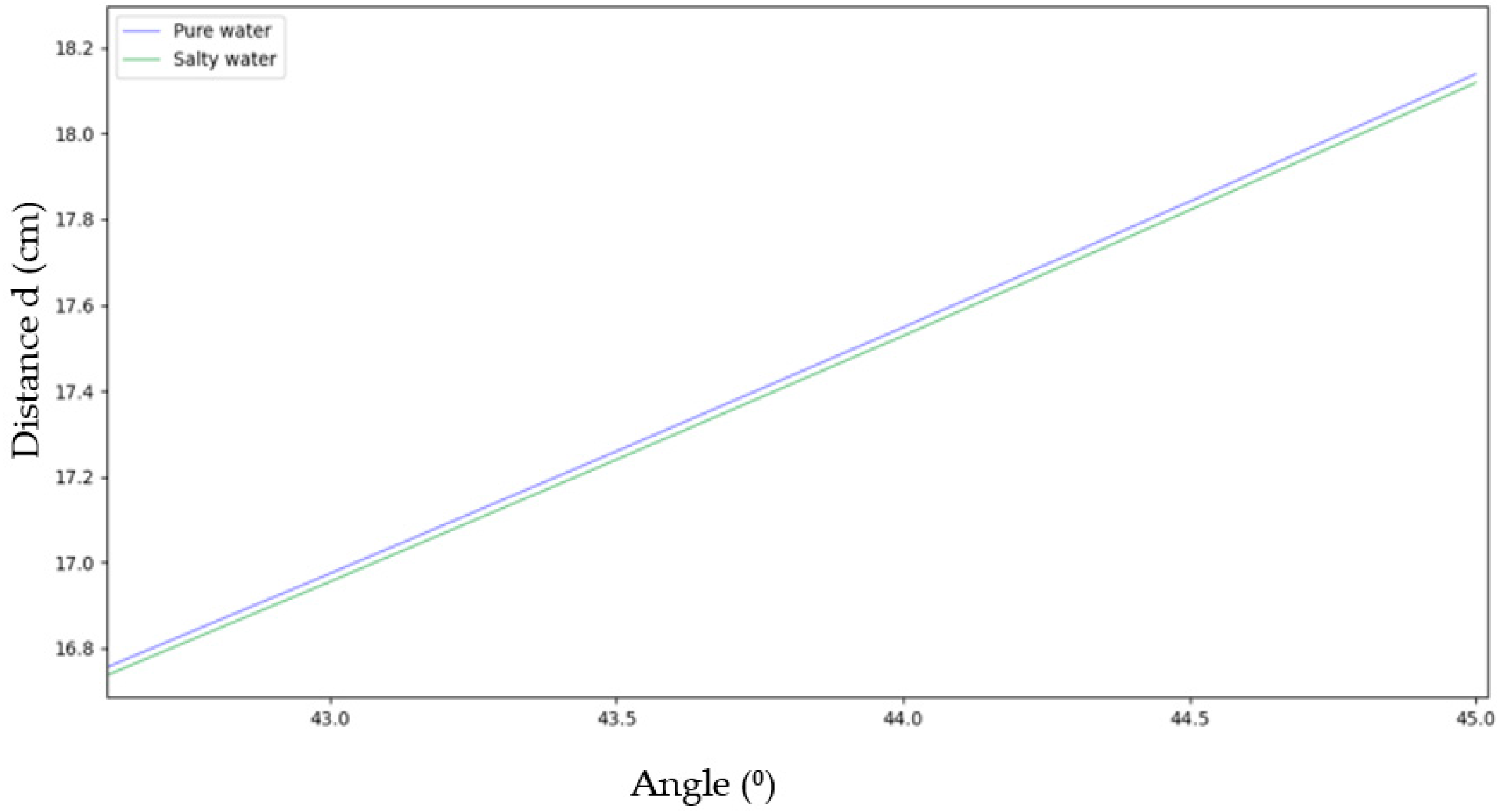
| 90 | Pure water (S = 0) | 73 | 17 |
| 90 | Salt water (S = 35%) | 66 | 24 |
Publisher’s Note: MDPI stays neutral with regard to jurisdictional claims in published maps and institutional affiliations. |
© 2022 by the authors. Licensee MDPI, Basel, Switzerland. This article is an open access article distributed under the terms and conditions of the Creative Commons Attribution (CC BY) license (https://creativecommons.org/licenses/by/4.0/).
Share and Cite
Mourched, B.; Ferko, N.; Abdallah, M.; Neji, B.; Vrtagic, S. Study and Design of a Machine Learning-Enabled Laser-Based Sensor for Pure and Sea Water Determination Using COMSOL Multiphysics. Appl. Sci. 2022, 12, 6693. https://doi.org/10.3390/app12136693
Mourched B, Ferko N, Abdallah M, Neji B, Vrtagic S. Study and Design of a Machine Learning-Enabled Laser-Based Sensor for Pure and Sea Water Determination Using COMSOL Multiphysics. Applied Sciences. 2022; 12(13):6693. https://doi.org/10.3390/app12136693
Chicago/Turabian StyleMourched, Bachar, Ndricim Ferko, Mariam Abdallah, Bilel Neji, and Sabahudin Vrtagic. 2022. "Study and Design of a Machine Learning-Enabled Laser-Based Sensor for Pure and Sea Water Determination Using COMSOL Multiphysics" Applied Sciences 12, no. 13: 6693. https://doi.org/10.3390/app12136693