1. Introduction
Data availability has left a drastically increasing competition between companies across all domains. In order for businesses to make sense of their data, there comes the need to employ machine learning specialists or data scientists with the proper background knowledge. However, many phases of most machine learning problems can be efficiently automated. The automation of such repetitive tasks will eventually lead to the reduction of human effort which is one of the main goals of machine learning in general.
In the past few years, new methods that enable domain experts to work with AI-supported technologies have emerged, these techniques usually require no background knowledge by using software tools to connect the experts with their work directly. This is similar to the work being conducted in automated machine learning (AutoML). Recent studies investigated the efficiency of the AutoML techniques [
1] applied by non-experts from various fields. Despite the easy-to-follow workflow, users expressed a need for a deeper understanding of the processing steps and results. Visualization is a straightforward way to overcome this issue, and it is also supported by studies [
2,
3].
Our objective is to introduce a user-friendly framework for domain experts that visually supports the understanding of the processing steps and leads toward proper evaluation of image classification and clustering tasks without requiring extensive knowledge of deep learning.
In this research, the close inspection and careful handling of the soldering-related industrial data were both prerequisites.
Visual inspection at each stage of the production line or in the quality control of the actual product is essential for the manufacturing efficiency of industries. The human workload is critical in this process since many industries still use conventional visual inspection methods and human labor instead of automation. When conventional approaches reach their limits, the commonly used automation concept is the contactless automatic optical inspection (AOI), which can have different hardware and software configurations, but most simply requires an image sensor (e.g., a camera), an illumination device, a computer for processing, a conveyor belt for transferring the products and an inspection algorithm [
4].
The use of commercially available AOI systems in solder joint inspection processes is a commonly used standard method according to the work of Metzner et al. [
5]. The authors revealed the limitations of such systems, which are rule-based implementation, general lack of flexibility to adapt to new cases, need for a high-level of domain knowledge for setup, and technological support during runtime. The research presented a deep learning supported solution, namely a convolutional neural network based classifier for classifying normal solder images and solder defects. After a detailed comparison and evaluation, the superior performance of the new method was concluded. As an outlook, the authors emphasized that obtaining the right amount and proportion of labeled training data is still one of the critical issues in the practical application of deep learning.
Deep learning has already been used to support automated industrial inspection in 2016, as shown in the publication by Weimer et al. [
6]. Instead of the commonly used hand-designed image processing solutions, they introduced a deep convolutional neural network (CNN) for the automatic generation of powerful features. The work emphasized that general optical quality control methods are adapted to controlled environments and fail on complex textures or noisy data, their performance also relies on human capabilities. Since there is a large variation in the visual appearance of defects, a modern automated visual inspection system must be able to handle this. Since deep neural networks learn from examples, a significant amount of training data is required, but only minimal prior knowledge of the problem domain, meaning that no domain expert knowledge is needed to develop a CNN-based visual inspection system.
Another real-world example of the practical application of deep learning image classification in visual inspection is the detection of cracks in concrete surfaces [
7]. The work presented a CNN-based approach with high accuracy classification performance and also showed that the domain knowledge of artificial intelligence specialists is essential to fine-tune the model appropriately.
The study by Dai et al. [
8] proposed a novel solder joint defect classification framework that incorporates deep learning and is potentially applicable to real-world AOI scenarios of solder joint inspection tasks. The authors’ motivation is that traditional inspection methods are still commonly used in modern factories, but their limitations make AOI techniques increasingly relevant. The paper describes in detail the three phases of AOI, which are image acquisition, solder joint localization, and classification.
The research of Wang et al. [
9] has drawn attention to the growing importance of visual quality control of products in all kinds of manufacturing processes. The study also highlighted that many factories still use traditional methods instead of automation to detect defects in products, these methods are expensive and labor-intensive, but due to the natural limitations of workers, efficiency is highly dependent on fatigue. This research has made it clear that there is an urgent need for novel automated defect detection systems in manufacturing processes. The authors implemented a CNN for image classification and successfully validated the approach on a simple benchmark dataset of defect-free and defective images. However, the paper did not consider a real-world example the proposed solution was also a CNN model, similar to the work of Metzner et al. [
5].
As previous works have shown, automating visual inspection is an essential step towards efficient production to ensure fast and reliable product quality control. The use of deep learning solutions leads to excellent performance, but the bottleneck to the uptake of the technology is a large amount of training data or annotation and the lack of comprehensive knowledge of AI.
In our proposed pipeline, beyond minimizing the labelling efforts, the domain experts may also identify misclassifications by trying more than one evaluating network that we put forth here. Thus, the proposed pipeline supports domain experts to independently evaluate their data without the in-depth involvement of AI specialists. We developed a prototypical pipeline jointly with a software tool called NIPGBoard used to conduct visual inception. The tool builds on the data projection benefits of the well-known TensorBoard visualization toolkit of TensorFlow [
10].
In contrast to the aforementioned works, one of our main goals was efficient clustering of soldering images for easier annotation, rather than filtering defective images. Due to their sheer number (≈75k) of samples in our database, it is difficult for the domain experts to label them by hand as it is a tedious and time-consuming process, meaning that an automated method is required. For this reason, we consider deep learning-based clustering techniques since they have become an influential trend in clustering methods and still have great potential. Another reason for considering these techniques would be that state-of-the-art deep learning architectures are available online with pre-trained weights on the ImageNet dataset [
11]. Therefore, by utilizing these pre-trained models, it is possible to extract latent space representations (embeddings) from the network and train an independent algorithm to create clusters based on the features captured by these representations for any required dataset, indicating that the clustering representations of the data maybe be efficient independently from the database. The only condition is that the images have to be resized to fit the pre-trained model input shape. Training a model to fit these representations can be done with or without any labels, meaning it is possible to label a subset of the overall dataset, making this problem somehow like a semi-supervised problem instead of a fully unsupervised task. Both methods have their advantages and disadvantages, but in general, they both may work well. Nevertheless, for high accuracy, a ratio of the data needs to be manually annotated by the experts. This ratio depends on the required precision, dataset complexity, number of unique categories, variations within each class, and the dataset distribution.
Deep clustering approaches and representation learning-based clustering techniques have gained popularity over traditional clustering methods in the last few years and have shown remarkable performance in unsupervised representation learning [
12].
Clustering is a fundamental unsupervised learning approach used in knowledge discovery and data science. Its principal purpose is to group data points based on their main attributes [
13] without access to the ground truth labels or prior knowledge of the data distributions, categories, or the nature of the clusters. It is also defined as the unsupervised classification of patterns (observations, data items, or feature vectors) [
14]. This means that the established groups could be much more than the required categories, as they can capture even the simplest variances within each class. On the other hand, supervised learning aims to find the correlation between the input and the output label by constructing a predictive model learning from a vast number of training examples, where each training example has a label indicating its ground truth output [
15].
Many researchers have published state-of-the-art deep learning neural networks with trained weights [
16,
17,
18,
19,
20,
21] on benchmarks datasets such as the ImageNet dataset, which contains a thousands of classes.
We intend to use both techniques to join their advantages in a kind of semi-supervised learning [
22]. Semi-supervised learning uses large amounts of unlabeled data and a small portion of labeled data to build better classifiers, meaning that it requires less human effort and gives higher accuracy [
23] than unsupervised learning approaches. Therefore, we can attempt to find the minimal amount of labeled data that still produces high accuracy.
In our implementation, we do not attempt to train any network, as it would require large computational efforts and special knowledge that the domain experts do not possess. Therefore, we will try the second approach by directly employing the feature space and using it in cluster construction to take advantage of the available pre-trained image classification convolutional neural networks. We train a Uniform Manifold Approximation and Projection (UMAP) model [
24] to reduce the dimensionality of the problem, effectively establishing the clusters between these images based on their feature space. New implementations tend to treat the clustering and the dimensionality reduction tasks jointly to learn what is known as cluster-friendly representations. These representations have shown that optimizing the two methods together improves the performance of both [
25].
Deep clustering techniques are powerful, but they usually suffer from several challenges. For instance, setting the optimal hyper-parameters for these techniques is not a trivial task [
26] as the recommended parameters are mainly benchmark-based on datasets such as MNIST [
27], and CIFAR-10 [
28] that do not reflect the complexity of real-world tasks. Whereas in our adaptation, the network is already trained and fine-tuned by a professional group of deep learning specialists. Nevertheless, we still have some parameters to optimize concerning the dimensionality reduction algorithm, such as the number of neighbors and iterations used in UMAP. Fortunately, these parameters are reasonably limited and easy to understand. In addition, running the algorithm requires a modest amount of resources only. Reducing the size of the data to be processed is a simple way to overcome this limitation. A small subset may be sufficient for fitting the model to obtain a reasonable performance, such as in our case, but careful selection is required to balance the data.
The other major issue is the lack of theoretical background and interpretability [
26], as explaining why and how these algorithms produce good results. Selecting the right pre-trained network for each dataset is also a challenge. It is often challenging to predict their behavior and performance for out-of-sample cases.
Our goal is to derive a method capable of effectively reducing the domain experts’ workload by minimizing the number of samples that require manual annotation. The proposed pipeline also helps individuals with little or no experience with AI to work and achieve the desired results. The main idea relies on utilizing deep clustering representation learning using pre-trained networks to achieve high-quality clusters without the need for deep learning specialists’ involvement. Also, by applying more than one network one may identify misclassifications and return them to experts for review and correction as we show. The introduced framework is based on a case study of a collaboration between AI specialists and domain experts on an image classification task on an industrial dataset.
2. Materials and Methods
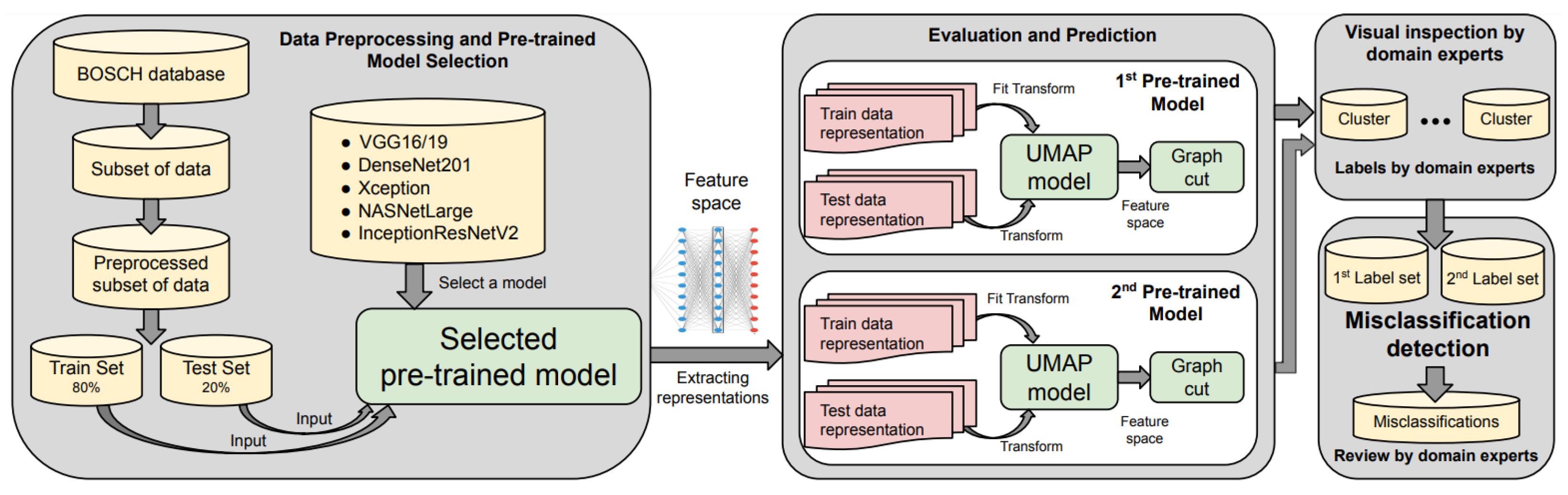
In this section, we introduce the pipeline for domain experts to accomplish a general image classification task. The practical scenario was carried out on an industrial dataset as part of academic-industrial cooperation. We propose a solution that automates the image clustering process entirely, prepares the data for easier annotation, provides visual explanation, and gives domain experts the power to find data clusters independently, with high precision.
First, the domain experts select random data points from the overall dataset. In our case, approximately 8% of the dataset was selected in the process. The data needs to be examined and processed appropriately to ensure that all the images are unique and have an appropriate format. Following the first step, the pre-processed dataset is to be divided into a training and a test subset. Ordinarily, it is 80–20% as one of the most common splits suggested by the literature. However, the ratio often depends on the problem at hand, the complexity of the data distribution, and other factors. For our case this split was sufficient given that it is a binary classification problem with a relatively balanced dataset and limited within-class variations for the two categories. Other more elaborate methods, such as k-fold cross-validation, can be used to estimate the error rate more accurately. Nonetheless, the purpose of the research is to ease the works of the experts, and avoid adding more complicated evaluation criteria.
The second component is the selection of a pre-trained deep learning architecture to work with. Recently there has been an arsenal of free, online available, and easily integrated pre-trained networks. These models include VGG16/19 [
16], DenseNet [
17], NASNet [
18], Inception [
19], InceptionResNet [
19], Xception [
20], EfficientNet [
21], ResNet [
29] and their variations.
Extraction of the representations of the train and test sets is done by feeding the sets to the pre-trained model to retrieve their corresponding feature space which we will also refer to as embedding.
Training and testing proceeds as follows. The latent representations of the train set are used to fit a UMAP model. This step can be accomplished with or without using the ground truth information. Using labels will improve the performance of the model by increasing the accuracy of the clusters. Nonetheless, labeling data is time and energy consuming, therefore a trade-off is required to achieve the highest possible accuracy with the minimal required manual annotation.
After obtaining the 2D or 3D embeddings produced by the UMAP model, the next step is the separation of the clusters from each other. In this processing phase, visual inspection can be performed using the NIPGBoard visualization tool.
The separation can be done by considering that all the data points form a fully-connected graph. The graph connections need to be minimized as the number of the edges is equal to . After minimizing the graph, we need to establish the boundaries between the clusters. This trained UMAP model is used to transform the latent representations of the test set into the UMAP space and the isolated clusters need to be checked independently by the domain experts by means of a few examples in each set.
Finally, one can use more than one evaluating network, compare the results and point to potential misclassifications that we detail later.
Figure 1 shows the pipeline steps as a flowchart.
2.1. Industrial Dataset
The joint research focused on deep learning supported evaluation of a large sized, soldering-related industrial dataset, provided by Robert Bosch, Ltd. (Bosch). As a concrete industrial example, in electronics manufacturing the soldering process refers to joining two or more metallic items together by melting and putting a filler metal into the joint. This filler metal is called solder and has a lower melting point than the adjoining metals. Soldering is utilized in many household devices and in-vehicle equipment. The reliability of solder joints is generally evaluated after long environmental testing, which is part of the product development process. Several methods are used for this process, including destructive techniques such as creating polished cross-sections and evaluating the internal structure of the solder joint.
This database represents cross-sections and other visual inspection images collected from different laboratories: pictures are taken under different lighting conditions, different camera parameters, and under different angles, indicating a difference in data distribution. The database does not have predefined rules about the capturing methodology. In addition, images are either captured using microscopes or ordinary photo cameras, showing electronic control units in whole or partially. These images happened to be collected over many years, are managed in a complex directory structure, and lack the proper labels.
Figure 2 shows example images from the Bosch dataset representing the two main image categories:
cross-section samples and the so called other recordings. These two image group names refer to the target categories of the classification task.
The data used in this task was randomly sampled from a set of a more comprehensive dataset (size of ≈75k). The domain experts had to randomly select images from the complete collection, which is stored in a complex directory structure. The selected data were manually renamed and labeled. This involved assigning each image one of the two given labels: either cross-section or other.
Even though there are only two distinct categories, each has multiple subclasses. The images in the other category are records of essential details and devices that are relevant in the Bosch laboratories. Such as parts and the boxes that contain the type of equipment. The cross-section images appear to have two main types: bright field and dark field. The aforementioned attributes are only general observations and these are not covering the overall characteristic of the dataset. The subset selected for the research was approximately 8% of the overall dataset.
The experts have labeled 6235 images. Out of this sample set 4159 belong to the cross-section category, and 2076 to the other visual inspection-related images. This random subset was not balanced, as it contained about twice as much cross-section data as the number of images in the other category. Although, this distribution represents the state of the full dataset, where the number of cross-section recordings is roughly twice the size of the other category. In general, the other category is more diverse, which might be problematic if the selected subset does not contain elements of each subclass. One can search for such examples by devising a method that searches for the most dissimilar (or least similar) images within the subset compared to the overall database.
2.2. Data Examination and Preprocessing
Before we proceed with the training process, potential issues related to the data collection characteristics need proper management. Since the dataset was provided by Bosch where the image recordings are stored in a complex structure, the data should be examined with simple scripts to ensure the proper quality and distribution for the forthcoming tasks. These preprocessing steps cover the removal of duplicated images and the examination and comparison of the similarities of the images.
2.2.1. Removing Duplicates
First, we need to ensure that the dataset does not contain redundant images. In this step, we examine whether an image appears multiple times or not. With the application of a simple, fast, and effective method, we checked the hash values of each image and compared them to each other. Thus we can investigate if two or more files having identical content under a different name are present in the dataset. As a result of the filtering, we removed the redundant data from the subset to be processed.
2.2.2. Examining Similarity
The second step is to examine the similarity distribution between all the images within the dataset to learn about data correlations. After investigating the dataset, we found that several pictures had similar latent space representations. This similarity factor is measured by taking the distance between the latent space representations of the images after normalizing or standardizing the images; in this case, images were divided by the maximum possible value of the pixels (255) as the standard image normalization method.
Comparison of the latent space similarities was carried out in feature space of the VGG19 model. A different pre-trained network could have been used, but since we are comparing the most similar images based on the extracted features of the model, then no notable gain would have been obtained from picking a different pre-trained model. We used the Euclidean distance between the representations of the images and concluded the following:
By setting a small distance threshold of 0.3 and less: 10 similar images were detected, meaning that these images have at least another significantly related sample in the dataset. For instance, one of the examples is shifted a few pixels from the other one. It is indistinguishable to the human eye, especially since the image had a large resolution, making these tiny details and differences hard to pick up by the experts.
For a threshold of 0.6 and less: 27 similar images were identified, 10 of them were the same as in the previous case, and the others had some minor differences. For instance, in some cases, one of the two images had measurements written on them.
By increasing the threshold to 1.0, we found 86 images. Some of the cases were the same as the previous ones. However, new instances emerged with significant differences. For example, two of the pictures were of the exact same device, one of them was with bolts, and the other one was not having bolts.
Based on these observations, the decision was to keep all the images as they will have no significant effect on the model performance or the measured accuracy. Additionally, given that this is how the original dataset is stored, we did not want to artificially influence or manipulate the data distribution. Nonetheless, such functionality might prove useful in other cases, this remains up to the industrial domain experts to decide when to use it.
2.3. Train and Test Sets
Almost any machine learning problem will need to have a separate set to ensure that model can generalize what it has previously learned into unseen data. Since we are utilizing clustering techniques to classify images into two general categories, we will need such a set as well.
Considering that we are using pre-trained models, the test set will only make a difference when applying the dimensionality reduction algorithms to the previously learned representations. Usually, keeping around 20% for the test set is an appropriate percentage, but it depends on the problem, the complexity of the issue, the size of the dataset, and many more factors that could influence the set size. Binary classification problems (as in this case) could require an even smaller test set, but in our case, there is a lot of diversity within each class.
Thus taking less than 20% may cause some of these variations to occur in the training set only. The train set of cross-section category contains 3322 images and the corresponding test portion has 837 examples. The other category holds 1666 samples for training and 410 images for testing purposes.
2.4. Selection of Deep Neural Network Models
Over the years, numerous architectures have been published with their weights, trained on massive datasets such as the ImageNet database. A common practice is to fine-tune these pre-trained weights on the required dataset instead of taking some randomly initialized weights, as the pre-trained networks have already proven their capabilities and constructed a common feature space. However, as we seek to connect the domain experts with their work directly, such an option is only feasible for a deep learning specialist but not suitable for the domain experts. Thus we needed to take a different approach to use these pre-trained models. The method that we will be using consists of extracting the pre-trained latent representations and treating these embeddings as features. These features will then serve as an input to one of the dimensionality reduction algorithms such as principal component analysis (PCA) and UMAP.
It is difficult to determine which architecture will yield the best result on a particular dataset. Even for AI professionals picking the best structure could sometimes be reduced to trial and error. Therefore, the domain experts will try a few architectures before finding the right one. Trying such models does not take much effort as they already have been trained.
In theory, with the help of NIPGBoard visualization interface, one only has to click a few buttons to examine these networks and evaluate their results.
One of the approaches to decide on the architecture is to start with the state-of-the-art networks that achieve the highest accuracy on the ImageNet dataset. Nevertheless, this method does not warrant that it will have the best result on the current dataset; it has a better chance to obtain the most favorable outcomes.
2.5. Extracting the Representations
After splitting the dataset and choosing a pre-trained architecture, the two sets of images (train and test portions) are inputted into that particular network. The output is one of the deep layers of the model. It is usually preferred to take the layer just before the softmax/output layer as it has a representation that was optimized for achieving high classification accuracies on the ImageNet dataset. The resulting representation is a two-dimensional matrix where each row is a vector representing the captured feature space of the corresponding image. We assume that the large number of ImageNet classes have many diverse features on this last layer suitable for discriminating novel classes and thus we expect high quality clusters.
After the extraction process, we used the representations of the training and test datasets for training a UMAP model with the corresponding labels that the domain experts provided and then testing it.
2.6. The UMAP Model
Uniform Manifold Approximation and Projection for Dimension Reduction (UMAP) is a manifold learning technique typically used for dimension reduction that results in an effective and scalable algorithm that can be effectively applied to virtually any real-world dataset. It is also competitive with other dimensionality reduction algorithms such as t-SNE [
30] for visualization quality and supposedly preserves more of the overall layout with excellent run time performance. Furthermore, UMAP has no computational constraints on embedding dimension, making it useful as a general-purpose dimension reduction technique for several machine learning problems. The algorithm makes three assumptions about the data. (i) A uniform distribution of the data on the Riemannian manifold, (ii) the Riemannian metric is locally constant (or can be approximated as such), (iii) and finally, the manifold is locally connected.
2.7. UMAP Model Training
Now that we have obtained the representations for both training and test sets they will be used to train a UMAP model with the corresponding labels that the domain experts provided. It is possible to train the model without labels as well, but omitting them will cause a noticeable decrease in accuracy. In other words, we could have only labeled the test set or even not have used any labels at all. However, then measuring the accuracy score would have been difficult. We would have needed to use other measurements such as the Silhouette index [
31] to get some indicator of the quality of the clusters.
Training is as follows: UMAP has several parameters that need to be fine-tuned, so we picked the ones that seemed of high relevance. Then used a grid search to get the best model within that limits of the search space. Often the results were not so much different from each other or the default parameters because the accuracy was already high.
2.8. UMAP Evaluation
There are several methods for evaluating the accuracy of the resulting clusters. Some of these techniques work with labeled or unlabeled datasets as well. But first, we need to transform the obtained train and test set representations into the UMAP space. After that, the evaluation process starts, and it is applied for both the train and test set independently, as we would like to know the training accuracy as well as the test accuracy. Additionally, this resembles the prediction part of the pipeline, where the unlabeled data need to be classified or clustered in a graph-based seperation.
After obtaining the 2D or 3D embeddings produced by the UMAP model, one can start to separate the clusters from each other. It is possible to achieve this step by different means. One of them is to build a graph, where the nodes are the data points, and the edges are the connections between these nodes. We consider the similarity to be in the inverse of the normalized adjacency distance matrix. Another method is to use the nearest neighbor approach, where each new data point is classified based on its K nearest neighbors.
The graph connections need minimization as the number of the edges are equal to , where n is the number of images in the set. It is done by one of two methods. The first method uses the minimal spanning tree, where only a single path will remain for connecting all of the nodes together. The other approach would keep the nearest neighbors of each node according to some pre-defined threshold. In the first approach, there is no discontinuity in the graph. Consequently, even points away from the cluster centers will be considered in the process. However, in the second approach, points that do not satisfy the distance threshold will be cut right from the start and are marked as outliers. Both methods have some advantages and disadvantages. We studied both methods and found minor differences due to the high quality of the clusters. We decided to use the minimal spanning tree due to its higher speed in the steps detailed below.
After minimizing the graph, we need to establish the boundaries between each cluster. We used community detection algorithms such as Girvan–Newman [
32], and Louvain [
33] that extract common elements from large-scale networks. Community structure, a general feature of most networks tries to find network nodes clustered more tightly into groups.
Between these groups, there are only loose connections [
32]. Girvan–Newman revolves around finding the community boundaries by using centrality indices. Instead of constructing a measure that tells which edges are most central to communities such as the hierarchical clustering method, Girvan–Newman focuses on the least central edges that are mostly in between communities. On the other hand, the Louvain algorithm is a simple computationally efficient heuristic method based on modularity optimization.
Multiple clusters or common regions form the output of the community detection and each cluster will have some general features common between the nodes. For simplicity and computational efficiency, we used the Louvain algorithm throughout this study.
The found groups need to be assigned labels for the train and test datasets independently. It is done by counting the number of labels for each category in all of the clusters individually, then assigning each cluster the dominant type in that group where dominance is determined solely based on the number of label occurrences. However, during prediction, the system provides the label of the closest cluster to the new sample. Depending on the parameter settings, there could be between 4–32 clusters for each model.
2.9. Misclassification Detection
In the current study, the aforementioned steps are all it takes to achieve high accuracy for this particular dataset. Nevertheless, our goal was to get a near-perfect accuracy without involving deep learning specialists too much or at all. Consequently, we needed a simple approach to detect misclassifications in the model. We have considered multiple strategies such as identifying out-of-distribution data or anomalies. However, training an anomaly detector is not trivial, there is no guarantee that anomalies will get misclassified or that a misclassification is an anomaly.
We note that the UMAP model is dealing with the representations of the pre-trained model, so the features captured by the latent space will highly depend on the model architecture and the data used for training that model, such as the ImageNet dataset. With this idea in mind, we hypothesize that different pre-trained networks may result in distinctive features. Training a dimensionality reduction algorithm such as UMAP on these features might result in a different set of misclassifications for different pre-trained networks. Therefore we used more than one network to detect possible misclassifications in the data. We can say that a data point is dubious when two models classify it differently, meaning they disagree on which class the data point belongs to. For the most accurate classification, we selected the two best performing pre-trained models.
Table 1 shows the common metrics of the tried algorithms on the test dataset which means in our case DenseNet201 (with 0.9992 accuracy) and Xception (with 0.9976 accuracy) were chosen. The accuracy value refers to the number of correctly classified images in relation to the total number of data instances. It has its best value at 1. More than one network is an ensemble-like approach that can be useful as they address certain issues of learning algorithms that output only a single hypothesis. For example, different networks may be stuck in different local minima of the problem space and a voting method can be advantageous as it could reduce the risk of not generalizing well to unseen data. An example is a recent Kaggle competition: the winner produced state-of-the-art results with 18 different networks combined into an ensemble [
34] and larger ensembles were also competitive. For a review on ensemble methods, see, e.g., [
35] and the references therein.
In our case, we can turn to the domain experts if models disagree and, due to the high quality of the clusters, a small number of networks (two in our case) is sufficient.
Our approach for using more than one network drastically reduces misclassifications by detecting potential errors in the models’ prediction. However, the more models introduced, the more clusters need to be labeled by the experts, and each model results in approximately 10–25 groups. More models will give rise to more misclassification candidates and this increases the experts’ work in the process. In turn, if the number of such candidates is too high then more elaborate ensemble learning based voting system using more networks can overcome the problem. There is trade-off between the required accuracy, the number of networks, and the amount of manual work that should be done.
2.10. Visual Inspection with NIPGBoard
To connect domain experts, technology and, deep learning professionals, we used the NIPGBoard software which was developed by the Neural Information Processing Group (NIPG) at Eötvös Loránd University in collaboration with Argus Cognitive company. NIPGBoard similarly to Tensorboard is a visualization interface with interactive functions. It uses the core features of the Tensorboard projector plugin, with additional algorithms and the ability to use pre-trained networks at the touch of a button, guaranteeing ease of use for domain experts.
The projection panel displays thumbnail versions of the data, called sprite images, after automatically applying one of the built-in dimension reduction techniques. The 3D position of the displayed data corresponds to the low-dimensional embedding of the hidden representations of the images, which are extracted using one of the deep neural networks. The user of the NIPGBoard tool can combine the available learning algorithms with the dimensionality reduction techniques. Displaying the results and switching between embeddings is an easy-to-use interface feature, so domain experts can gain comprehensive knowledge about the data and the selected methods. Labels can be displayed for each piece of data, and label-based colour overlays can be added to the images to provide further information on quality of the clusters. Label-based colour overlays also show the effectiveness of clustering by visual inspection of data in the embedding space without additional AI expert guidance.
In the course of our work, we have incorporated additional functions into the software to make the work of the expert easier.
Figure 3 shows the interface of the NIPGBoard visualization tool with the loaded Bosch data.
4. Discussion
For experts with no experience in training deep networks, observing the evaluation of training and test data can provide useful knowledge.
Table 2 summarizes the pre-trained model performances on the training set. It is common for train data to have higher values than test data. As
Table 1 shows DenseNet201 has the best results for the test set, even though it is not the best performing model on the ImageNet among the ones that we have tested.
In addition to the numerical assessment, visualizations also give an indication of a properly constructed pipeline.
Figure 4 and
Figure 5 show that the data split was appropriate and highlights minor differences between the pre-trained models.
As it is shown in
Table 1 and
Table 2, the difference between the worst performing model VGG19, and the best performing model DenseNet201 is less than
. This phenomenon does not imply that DenseNet201 will always perform better than the other models for every case. We conduct that DenseNet201 has a good chance of performing well on similar datasets. Consequently, this also suggests that VGG19 will not perform well on a similar dataset. This experience can be gained by the domain expert themselves without any prior knowledge of the underlying architecture of the models.
Simple methods can support the work of domain experts to further improve data management tasks beyond labelling. For example, one can search for images or groups of images similar to a given image by measuring the distances between latent representations of images that can be incorporated into our pipeline. Another approach would be to search for anomalies by finding the least similar images in the dataset, or images representing a rare subcategory.
Generative Adversarial Networks (GANs) [
36] and Variational Autoencoders (VAEs) [
37] are becoming increasingly popular in anomaly detection tasks. The use of these algorithms is a promising opportunity for further improvements to expand our pipeline. Yet, the integration of such methods need care as they may involve training and need artificial intelligence specialists.
Although the case we studied brought about high-quality results, there are some possible limitations to it. For instance, it heavily relies on pre-trained models for feature extraction, meaning those features are extracted from the ImageNet dataset tuned for the classes of the dataset. In turn, the selection of the final layer could not be the optimal strategy for all datasets. However, in the case of this particular cooperation, this technique achieved the excellent results. It is hard to predict how the method will perform on other datasets. Another aspect that could be considered a downside is the need for human intervention in various stages of the pipeline. The current methodology design allows the experts to directly examine and interact with the data to decide the best course of action based on their experience. However, if the extreme high level of accuracy is not required, such careful examination could be deemed unnecessary.
5. Conclusions
We developed a pipeline for the domain experts assuming that they may not have comprehensive knowledge about deep learning AI methods. We used the pipeline to solve a soldering data classification task. In this pipeline, we took advantage of pre-trained models, clustering of the feature maps of deep networks, and misclassification detection using more than one network.
Our goal was overcome the bottlenecks in academic-industrial collaborations by separating the tasks of the AI specialists and the domain experts and simplifying the tasks for the latter by automatically labelling data while achieving high accuracy with as little manual work as possible. This separation is motivated by studies pointing out that solving a problem using deep learning is traditionally still a task for AI specialists. Bottlenecks include the struggle with communication misunderstandings and knowledge gap between the expertise of the two fields. We showed that direction of separating the tasks using our pipeline is promising.
For domain experts, one novel way is to use the so-called AutoML system, but as the referred studies emphasized, confidence and positive user experience depend heavily on understanding such systems. We also used embedding into 2D or 3D, clustering of the embeddings and the belonging visualisations for helping in the steps towards the final results.
The documented evaluation pipeline provides compact and generic guidance and visual representations for domain experts on how to manage data properly and take advantage of deep learning methods. We had to request some annotation work from the domain experts followed by simple preprocessing steps, easily accessible pre-trained models, visual and numerical comparison, and explanation of why model selection may be appropriate.
We also tried to point out potential misclassifications by means of more than one pre-trained network: disagreements between their classification results can serve as indications. Dubious samples were sent back to the experts for review. We noted that a larger set of pre-trained networks could lead to a voting system called ensemble learning. Our approach was able to achieve near-perfect accuracy on the test set with only data labeled by domain experts.


