Efficiently Detecting Non-Stationary Opponents: A Bayesian Policy Reuse Approach under Partial Observability

Abstract

In multi-agent domains, dealing with non-stationary opponents that change behaviors (policies) consistently over time is still a challenging problem, where an agent usually requires the ability to detect the opponent’s policy accurately and adopt the optimal response policy accordingly. Previous works commonly assume that the opponent’s observations and actions during online interactions are known, which can significantly limit their applications, especially in partially observable environments. This paper focuses on efficient policy detecting and reusing techniques against non-stationary opponents without their local information. We propose an algorithm called Bayesian policy reuse with LocAl oBservations (Bayes-Lab) by incorporating variational autoencoders (VAE) into the Bayesian policy reuse (BPR) framework. Following the centralized training with decentralized execution (CTDE) paradigm, we train VAE as an opponent model during the offline phase to extract the latent relationship between the agent’s local observations and the opponent’s local observations. During online execution, the trained opponent models are used to reconstruct the opponent’s local observations, which can be combined with episodic rewards to update the belief about the opponent’s policy. Finally, the agent reuses the best response policy based on the updated belief to improve online performance. We demonstrate that Bayes-Lab outperforms existing state-of-the-art methods in terms of detection accuracy, accumulative rewards, and episodic rewards in a predator–prey scenario. In this experimental environment, Bayes-Lab can achieve about 80% detection accuracy and the highest accumulative rewards, and its performance is less affected by the opponent policy switching interval. When the switching interval is less than 10, its detection accuracy is at least 10% higher than other algorithms.

1. Introduction

Recently, deep neural networks have provided excellent performance in image recognition [1], pattern recognition [2], and security [3,4,5]. They are usually combined with reinforcement learning (RL) and have achieved great success [6,7,8,9]. Many advanced deep RL algorithms have been proposed and used to solve complex decision-making problems such as game playing [9,10], robotics [11,12,13,14], and autonomous driving [15,16,17,18]. In multi-agent systems [19,20], if an opponent’s policy is fixed, the agent can treat it as part of the stationary environment and learn the response policy using single-agent RL algorithms [21,22,23]. However, in many cases, the opponent’s behaviors may change over time and affect the objectives of the others, which implies a non-stationary environment [24]. As a result, it is essential for the agent to adapt its policy by taking into account the non-stationary opponent [25,26,27,28], which is regarded as the second sophisticated challenge categorized in [26]. In this paper, we focus on dealing with the non-stationary opponents in a partially observable environment, where we control an agent with a limited horizon and the other agents (opponents) select their fixed policies from a policy library. In our setting, the controlled agent is required to reason about the opponent’s policy and adjust its policy to achieve optimal rewards. One effective way to address the non-stationarity is opponent modeling [22,27,29,30]. According to [30], the opponent modeling methods can be divided into implicit modeling and explicit modeling.

A natural idea for implicit modeling is to use deep neural networks to encode the opponent’s policy features [27,29,31,32]. Specifically, such models usually consist of two networks [33]: one is to extract the latent policy features from supervision signals such as the opponent’s actions [31], goals [34], and beliefs [27], and the other learns the response policy by taking into account these policy features. The deep reinforcement opponent network (DRON) [29] uses an additional network to extract the opponent’s policy features, and it incorporates a mixed-of-expert structure with a deep Q-network (DQN) [35] to handle different opponent policies. However, it cannot guarantee optimality against each particular opponent’s policy and assumes that the agent can observe the opponent’s actions. Deep policy inference Q-network (DPIQN) [36] learns policy features directly from the opponent’s raw observations. These features are learned by auxiliary tasks that provide additional supervision signals, such as the opponent’s actions. Self-other modeling (SOM) [34] proposes using the agent’s policy to predict the opponent’s goal. Despite its simplicity, it takes longer to train, as an additional optimization step is required to consider the opponent’s actions. Most studies reviewed here assume that the opponent’s observations and actions can be accessed during online interactions. However, this assumption is unlikely to hold in practical scenarios. To address this problem, local information agent modeling (LIAM) [37] first proposed the use of a variational autoencoders (VAE) [38] model to learn the opponent’s policy features in RL. This method can extract the hidden opponent features during training conditioned only on the agent’s local observations. In other words, it does not require the opponent’s local information during execution. A mutual limitation of the above studies is that they cannot reuse the existing offline response policies to accelerate online decisions for lacking explicit opponent categorization. When the opponent switches between several known policies, the agent has to learn new response policies from scratch, which is inefficient [30].

The above problem is motivated by many application domains where the agent requires fast online decision making [39]. For example, a service robot has to interact with people with different policies (behaviors). For each of these policies, the robot needs to use an appropriate response policy to achieve optimal performance on the task [40]. It is very inefficient if the robot has to learn new coping strategies from scratch during online interactions. More commonly, the robot maintains an offline response policy library and reuses the response policies directly based on human online behaviors. Compared with the implicit modeling methods that can only learn the response policy from scratch during online interactions, our algorithm can reuse the offline learned policy to accelerate online decisions using explicit modeling methods.

One feasible direction for implementing explicit modeling is to exploit offline knowledge to improve online performance [39]. Type-based reasoning methods [30,41] assume that the opponent switches between several known types and the agent maintains a prior belief about the probability distribution of the opponent’s types. During online interactions, the belief is updated based on any task-related signals, and then the agent can reuse the existing response policy based on the updated belief. Bayesian policy reuse (BPR) [39] is an explicit opponent modeling framework based on type-based reasoning. It was initially applied to single-agent domains, where the agent can detect task types and reuse the learned best response policies when faced with multiple tasks. Regarding different opponent’s policies as different task types in BPR, BPR+ [40] first extended BPR to multi-agent scenarios to detect dynamic changes in the opponent’s policies. In addition, Bayes-Pepper [25] combines BPR with Pepper [42] to improve detection accuracy by using the opponent’s state–action pairs as an additional signal during belief updating. However, as table-based algorithms, BPR+ and Bayes-Pepper are spatially inefficient and even infeasible when dealing with complex scenarios. To overcome this problem, Deep BPR+ [43] proposes using a deep neural network as a value function approximator and an opponent model, which can be used to rectify the belief model in BPR+ to improve the detection accuracy. However, Bayes-Pepper and Deep BPR+ may suffer from incomplete opponent information. The above algorithms [22,23,40,43] assume that the opponent switches randomly among a class of stationary policies, but the opponent may be equally capable of reasoning, and thus adopts a more complex policy-switching approach. To address this issue, Bayesian theory of mind on policy (Bayes-ToMop) [44] assumes that the opponent also uses BPR. However, Bayes-ToMop needs to detect whether the opponent is using BPR through additional interactions when the opponent switches strategies randomly, which can be extremely time-consuming. Most BPR-based algorithms reviewed here assume that the agent can observe the opponent’s local information during online interactions, including its observations and actions. In practice, many tasks are characterized by partial observability, in which the agent can only obtain incomplete and uncertain observations about the opponent, making accurate policy detection more challenging.

In this work, we consider how to act optimally against non-stationary opponents that switch among several stationary strategies under partial observability. According to [45], a strength of VAE is that it can reason about the opponent’s policies without the opponent’s local observations. However, this method cannot reuse the learned response policies during online interactions for lacking explicit classification of the opponent’s policies. On the contrary, the BPR-based methods explicitly classify the opponent’s policies, and the optimal learned response policies can be reused during online interactions. However, most BPR-based methods require the opponent’s local observations to accurately identify the opponent’s policies. We consider that it is possible to combine these two forms of modeling to improve online performance under partial observability. Specifically, we perform an explicit opponent categorization and reuse the learned response policies without the opponent’s local information. We follow the centralized training with decentralized execution (CTDE) paradigm and propose an algorithm called Bayesian policy reuse with LocAl oBservations (Bayes-Lab), which incorporates VAE into BPR. Specifically, we train VAE during the offline phase to extract the latent opponent’s policy features only based on the agent’s local observations, and then use VAE to reconstruct the opponent’s actions during online interactions. In addition, we collect the reconstructed actions and episodic rewards to fit the reconstruction accuracy model, planning similarity model, and performance model, which are defined as Gaussian distributions. Using the generated models, we update the agent’s belief about the opponent’s types during the online phase. Finally, we reuse the best response policy based on the updated belief. Compared with most BPR-based algorithms [22,23,40,43,44] that infer the opponent’s policy from their behaviors, Bayes-Lab can track the opponent’s policy only conditioned on the agent’s local observations.

The most significant contribution of Bayes-Lab is that it can efficiently detect the non-stationary opponents under partial observability and accurately reuse the offline response policies to improve the online performance. The main novelty of this paper is as follows: (1) An opponent model is introduced to reconstruct the opponent’s local observations only based on the agent’s local observations. Bayes-Lab uses VAE as an opponent model to learn the relationship between the agent’s local observations and the opponent’s local observations. Then, the learned opponent model can be used to reconstruct the opponent’s actions under partial observability. (2) An offline learning architecture is introduced to simultaneously learn the response policy and the opponent model. Bayes-Lab uses VAE to extract the opponent’s policy features which are integrated with the agent’s observations to learn the response policy. The advantage of this architecture is that each opponent’s policy can correspond to an optimal response policy and a specific opponent model, which is essential for detecting the opponent’s type and reusing the response policy. (3) Bayes-Lab is the first to propose integrating VAE as an opponent model into BPR. Specifically, it combines the ability of BPR to improve online performance by using offline knowledge with the capability of VAE to reason about the opponent’s behaviors under partial observability. It can continuously infer the opponent’s policies during online interactions without the opponent’s local observations. Compared with other BPR-based methods that can only be used in the globally observable environment, Bayes-Lab can effectively apply BPR in the partially observable environment. (4) The reconstruction accuracy model and planning similarity model are introduced to improve the detection accuracy during online interactions. Bayes-Lab can use these models to detect the opponent’s policy and whether or not the opponent’s actions can be observed.

The rest of the paper is organized as follows: Section 2 presents the formal model of RL, BPR, and VAE. Section 3 introduces the proposed Bayes-Lab algorithm. Section 4 presents a validation environment, experimental settings, and corresponding experimental results. Section 5 concludes our contributions and problems that need to be solved.

2. Preliminaries

2.1. Reinforcement Learning

An RL task can be modeled as an MDP [24,46], which consists of a 4-tuple $〈\mathcal{S},\mathcal{A},\mathcal{P},\mathcal{R}〉$, where $\mathcal{S}$ is a finite set of states, $\mathcal{A}$ is a finite set of actions, $\mathcal{P}:\mathcal{S}\times \mathcal{A}\times \mathcal{S}\mapsto \left[0,1\right]$ is a transition function which describes the probability of the next state $s^{\prime }\in \mathcal{S}$, after taking action $a\in \mathcal{A}$ in state $s\in \mathcal{S}$, and $\mathcal{R}:\mathcal{S}\times \mathcal{A}\times \mathcal{S}\mapsto \mathbb{R}$ is a reward function which returns a scalar value conditioned on two consecutive states and the intermediate action. A policy function $\pi \left(a\left|s\right.\right)$ describes the probability distribution of choosing a in state s. An optimal policy can be learned by maximizing the state-value function or the action-value function. The state-value function is usually defined as $V^{\pi }\left(s_t\right)={\mathbb{E}}_{\pi }\left[{\sum }_{i=t}^H{\gamma }^{i-t}{r}_t\left|s=s_t\right.\right]$, which represents the expected rewards for visiting state and following policy $\pi$ thereafter. Similarly, the action-value function is defined as $Q^{\pi }\left(s_t,a_t\right)={\mathbb{E}}_{\pi }\left[{\sum }_{i=t}^H{\gamma }^{i-t}{r}_t{\left|s=s_t,a=a\right.}_t\right]$, which describes the expected rewards for taking action a when visiting state s and keeping policy $\pi$ throughout, where $0\le \gamma \le 1$ is a discount factor, and H is the finite horizon of the episode.

In this paper, we use advantage actor–critic (A2C) [7] to learn the response policy. The opponent’s policy will remain fixed until the agent learns the optimal response policy. Suppose there is a policy network ${\pi }_{\theta }$ with parameter $\theta$ and a value network $V_{\varphi }$ with parameter $\varphi$. A2C updates the network parameters as follows:

$$\begin{array}{c}\hfill \begin{array}{c}\hfill \underset{\theta ,\varphi }{min}{\mathbb{E}}_B\left[-\widehat{A}log{\pi }_{\theta }\left(a\left|s_t\right.\right)+\frac{1}{2}{\left(r+\gamma V_{\varphi }\left(s_{t+1}\right)-V_{\varphi }\left(s_t\right)\right)}^2\right]\end{array}\end{array}$$

(1)

where $B={\left\{\left(s_t,a_t,r_t,s_{t+1}\right)\right\}}_{t=0}^{t=H}$ is the batch of transitions, and $\widehat{A}$ is the basic advantage term.

2.2. Bayesian Policy Reuse

BPR [39] was originally proposed as a framework for an agent to determine the best response policy to execute when facing an unknown task in Markov Decision Process (MDP) [46,47]. Given a set of previously solved tasks $\mathcal{T}$ and current task ${\tau }^{*}$, the agent is expected to detect the type of task efficiently and reuse the optimal response policy ${\pi }^{*}$ from the policy library $\mathrm{\Pi }$ accordingly based on the observation signal $\sigma$ within a small number of interactions. The signal $\sigma$ can be any information related to the performance of a policy (e.g., episodic rewards, encountered state–action–state tuples). In addition, a performance model $P\left(U\left|\tau \right.,\pi \right)$ is a probability distribution over the utility U generated by applying a policy $\pi$ to a previously solved task $\tau$. BPR uses the concept of belief $\beta$, which is a probability distribution over the tasks $\mathcal{T}$, to estimate the matching degree between ${\pi }^{*}$ and the known tasks based on the signal $\sigma$. After each trial episode, ${\beta }^k\left(\tau \right)$ is updated using a Bayes’ rule as follows:

$$\begin{array}{c}\hfill \begin{array}{c}\hfill {\beta }^k\left(\tau \right)=\frac{P\left({\sigma }^k\left|\tau ,{\pi }^k\right.\right){\beta }^{k-1}\left(\tau \right)}{{\sum }_{{\tau }^{\prime }\in \mathcal{T}}P\left({\sigma }^k\left|{\tau }^{\prime },{\pi }^k\right.\right){\beta }^{k-1}\left({\tau }^{\prime }\right)}\end{array}\end{array}$$

(2)

where ${\beta }^{k-1}\left(\tau \right)$ is the belief after episode $k-1$. In addition, belief updating can be regarded as identifying task types. For example, suppose the agent’s policy library includes two learned response policies, ${\pi }_1$ and ${\pi }_2$, which are used to handle tasks ${\tau }_1$ and ${\tau }_2$, respectively. If the agent uses ${\pi }_1$ to interact with an unknown task which is one of ${\tau }_1$ or ${\tau }_2$, the agent will receive a signal $\sigma$ that can be combined with the performance model P to detect the task type. Specifically, $P\left(\sigma \left|{\tau }_1,{\pi }_1\right.\right)$ reflects the possibility that the unknown task is ${\tau }_1$. Similarly, $P\left(\sigma \left|{\tau }_2,{\pi }_1\right.\right)$ reflects the possibility that the unknown task is ${\tau }_2$. By comparing $P\left(\sigma \left|{\tau }_1,{\pi }_1\right.\right)$ and $P\left(\sigma \left|{\tau }_2,{\pi }_1\right.\right)$, the agent can identify the unknown task type. Moreover, the received signal will be different if the task switches from one to another, resulting in changes in the performance model. As a result, the agent’s belief $\beta \left(\tau \right)$ can be rectified based on Equation (2), leading the agent to reselect its response policy.

Several variants of BPR with exploration heuristics are available to choose the optimal response policy, among which BPR using an expected improvement (BPR-EI) presents the best performance. Assume that $\overline{U}={max}_{\pi \in \mathrm{\Pi }}{\Sigma }_{\tau \in \mathcal{T}}\beta \left(\tau \right)E\left[U\left|\tau ,\pi \right.\right]$ is the optimal estimated utility following the existing belief. BPR-EI selects the policy most likely to lead to any utility improvement $\overline{U}<U^{+}<U^{max}$ as follows:

$$\begin{array}{c}\hfill \begin{array}{c}\hfill {\pi }^{*}=\underset{\pi \in \mathrm{\Pi }}{\mathrm{argmax}}{\int }_{\overline{U}}^{U^{max}}\sum {}_{\tau \in \mathcal{T}}\beta \left(\tau \right)P\left(U^{+}\left|\tau ,\pi \right.\right)d{U}^{+}\end{array}\end{array}$$

(3)

2.3. Variational Autoencoders

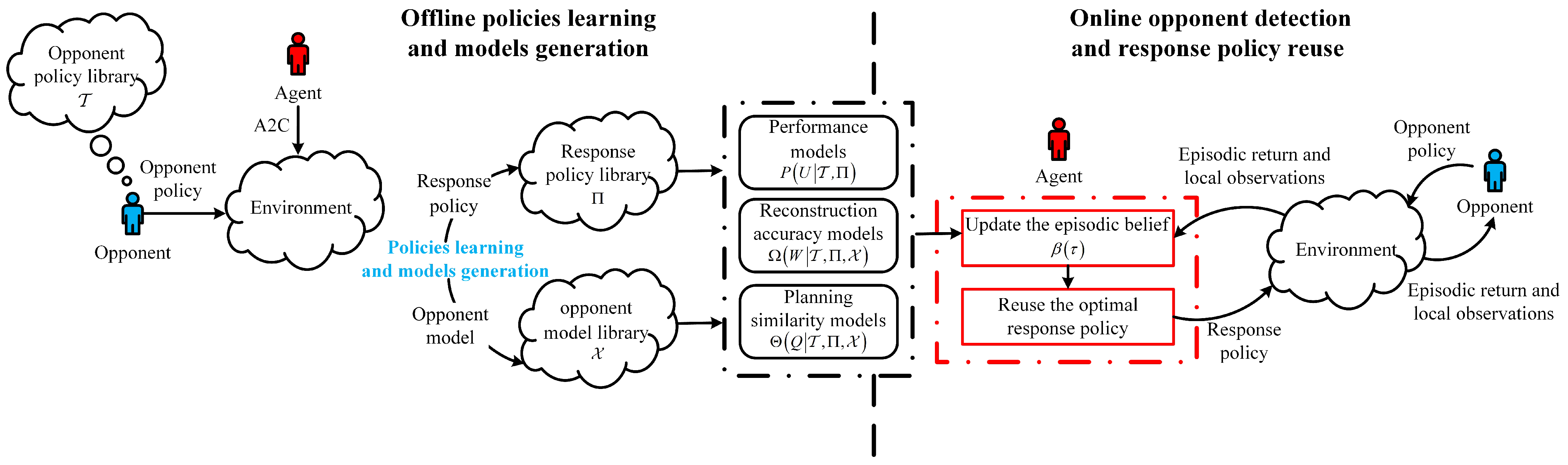
In recent years, variational autoencoders (VAE) [38] have become one of the most popular methods for unsupervised learning of complex distributions [48]. The VAE model uses deep neural networks [49] as standard function approximators and can be trained using stochastic gradient descent [50]. In image generation [48,51], the VAE model has been proven to be effective in generating wide varieties of complex data. In RL [24], many works use VAE to learn low-dimensional representations of the environment, leading to significant improvements [52,53].

Assume that samples from a data set $x\in \mathcal{X}$ are generated from some hidden (latent) random variables z based on a generative distribution $p_{\alpha }\left(x\left|z\right.\right)$ with unknown parameters $\alpha$. The prior distribution over the latent variables z is a Gaussian distribution with $\mathbf{0}$ mean and unit variance $p\left(z\right)=\mathcal{N}\left(z;\mathbf{0},\mathit{I}\right)$. The VAE model learns a variational parametric distribution $q_{\sigma }\left(z\left|x\right.\right)=\mathcal{N}\left(z;\mathbf{\mu },\Sigma ,\sigma \right)$ to approximate the true posterior probability $p\left(z\left|x\right.\right)$. In addition, the approximation of the true posterior starts with the computation of the KL divergence $D_{KL}\left(q_{\sigma }\left(z\left|x\right.\right)∥p\left(z\left|x\right.\right)\right)$. Moreover, the lower bound of evidence $logp\left(x\right)$ (ELBO) is derived as follows:

$$\begin{array}{c}\hfill \begin{array}{c}\hfill logp\left(x\right)\ge {\mathbb{E}}_{z\sim q_{\sigma }\left(z\left|x\right.\right)}\left[log{p}_{\alpha }\left(x\left|z\right.\right)\right]-D_{KL}\left(q_{\sigma }\left(z\left|x\right.\right)∥p\left(z\right)\right)\end{array}\end{array}$$

(4)

A VAE model is composed of an encoder and a decoder. Specifically, the encoder receives samples and generates a Gaussian variational distribution $p\left(z\left|x;\sigma \right.\right)$. The decoder accepts the samples generated by the Gaussian variational distribution and reconstructs the original input x. In addition, the VAE model is usually trained by a parameterization trick [38]. $\beta$-VAE [54] proposes taking advantage of the parameter $\beta$ which is positive to control the balance between the KL divergence and the reconstruction loss:

$$\begin{array}{c}\hfill \begin{array}{c}\hfill L\left(x;\sigma ,\alpha \right)={\mathbb{E}}_{z\sim q_{\sigma }\left(z\left|x\right.\right)}\left[log{p}_{\alpha }\left(x\left|z\right.\right)\right]-\beta D_{KL}\left(q_{\sigma }\left(z\left|x\right.\right)∥p\left(z\right)\right)\end{array}\end{array}$$

(5)

3. Bayes-Lab

An overview of Bayes-Lab is shown in Figure 1. It consists of two stages: (1) an offline stage used to learn the response policies and generate the corresponding models and (2) an online stage for opponent’s policy detection and optimal response policy reuse. The left part presents the process of learning a new response policy $\tau \in \mathcal{T}$ and the corresponding opponent model $x\in \mathcal{X}$ and generating the performance model $P\left(U\right|\mathcal{T},\mathrm{\Pi })$, the reconstruction accuracy model $\mathrm{\Omega }\left(W\left|\mathcal{T},\mathrm{\Pi },\mathcal{X}\right.\right)$, and the planning similarity model $\mathrm{\Theta }\left(Q\left|\mathcal{T},\mathrm{\Pi },\mathcal{X}\right.\right)$. The right part describes the process of belief update and policy reuse during online interactions. The episodic belief $\beta \left(\tau \right)$ is used for opponent policy detection and optimal response policy reuse, and it is updated based on episodic returns and the agent’s local observations. In addition, each model generated in the offline process remains fixed in the online process, and the agent can constantly update the episodic belief through these models. With the change of the online signals, such as the episodic rewards and the agent’s local observations, the episodic belief calculated by offline models will be different, which can be used to track the change in the opponent’s behaviors.

During the offline stage, the agent interacts with each opponent’s policy to learn the corresponding response policy and the opponent model. In addition, the agent is also required to fit the performance models, reconstruction accuracy models, and planning similarity models, which are defined as Gaussian distributions. During the online stage, the agent incorporates the generated models to update the belief about the opponent’s types at the end of each episode, and then reuses the best response policies with the updated belief.

In the following sections, we denote the agent’s local observations within an episode by ${\phi }_1=\left(o_1^{*},a_1^{*}\right)$, where $o_1^{*}={\left\{o_{1,t}\right\}}_{t=0}^{t=H}$ and $a_1^{*}={\left\{a_{1,t}\right\}}_{t=0}^{t=H}$ are the agent’s observations and actions, respectively, and H is the finite horizon of the episode. Similarly, the opponent’s local information within an episode can be defined as ${\phi }_{-1}=\left(o_{-1}^{*},a_{-1}^{*}\right)$. Moreover, the opponent’s actions reconstructed by the opponent model within an episode can be referred to as $a_{-1,recon}^{*}$.

3.1. Offline Policy Learning and Model Generation

During the offline stage, Bayes-Lab first needs to learn the response policy $\pi$ and the opponent model x and then use them to constitute the response policy library $\mathrm{\Pi }$ and the opponent model library $\mathcal{X}$, respectively. In addition, we use the VAE networks to represent the opponent model. As shown in Figure 2, Bayes-Lab updates the A2C networks and the VAE networks simultaneously, and the VAE networks consist of an encoder and a decoder. The encoder learns a variational Gaussian distribution $\mathcal{N}\left({\mathbf{\mu }}_{\sigma },{\Sigma }_{\sigma }\right)$ with parameters $\sigma$ and is denoted as $q_{\sigma }\left(z\left|{\phi }_1\right.\right)$, which is used to approximate the true posterior distribution $p\left(z\left|{\phi }_{-1}\right.\right)$. The approximate posterior distribution $q_{\sigma }\left(z\left|{\phi }_1\right.\right)$ can map the agent’s local observations ${\phi }_1$ to a hidden variable space $\mathcal{Z}$ from which the hidden variable z is sampled as the representation of the current opponent policy. In addition, the KL divergence $D_{KL}\left(q_{\sigma }\left(z\left|{\phi }_1\right.\right)∥p\left(z\left|{\phi }_{-1}\right.\right)\right)$ is used to measure the similarity between the approximate posterior distribution and the real posterior distribution.

The decoder learns a generative distribution $p_{\alpha }\left({\phi }_{-1}\left|z\right.\right)$ with parameters $\alpha$ that maps the hidden variable z to the opponent’s local information ${\phi }_{-1}$, which is used as a supervision signal to update the encoder–decoder networks. As a result, the opponent model can reconstruct ${\phi }_{-1}$ conditioned only on ${\phi }_1$. Moreover, we use the $MM{D}^2$ distance [55,56] for regularization. The loss of the encoder–decoder networks is formulated as follows:

$$\begin{array}{c}\hfill \begin{array}{c}\hfill \mathcal{L}\left({\phi }_{-1},{\phi }_1;\alpha ,\sigma \right)=-{\mathbb{E}}_{z\sim q_{\sigma }\left(z\left|{\phi }_1\right.\right)}\left[log{p}_{\alpha }\left({\phi }_{-1}\left|z\right.\right)\right]+\lambda D_{MMD}\left(q_{\sigma }\left(z\left|{\phi }_1\right.\right)∥p\left(z\right)\right)\end{array}\end{array}$$

(6)

where $\lambda$ is a scaling parameter.

In the original A2C algorithm, the input of the policy networks is only the agent’s observations, and the obtained policy can be expressed by $\pi \left(a\left|o_1\right.\right)$. Obviously, it cannot be directly applied in a multi-agent environment for not considering the impact of the opponent’s policy on its policy. To explicitly consider the coexisting opponents in the environment, we propose using the latent variable z, which is sampled as the low-level feature of the current opponent policy. Specifically, the agent’s observation $o_1$ augmented with z can be used as input signals to update the A2C networks, and the learned policy can be expressed by $\pi \left(a\left|o_1,z\right.\right)$. We emphasize that the VAE networks are updated by supervised learning, while the A2C networks are updated by reinforcement learning. Therefore, A2C is a separate network, not another decoder. One advantage of this architecture is that each opponent’s policy ${\tau }_i$ can correspond to an optimal response policy ${\pi }_i$ and a specific opponent model $x_i$, which is essential for reusing the response policies based on the opponent types. Although A2C and VAE are updated simultaneously, they use different optimizers and learning rates. As a result, the loss generated by A2C will not affect the parameters of VAE through back-propagating the gradient. Given a batch of the agent’s behaviors data, the objective of A2C is:

$$\begin{array}{c}\hfill \begin{array}{c}\hfill \begin{array}{cc}\hfill & {\mathcal{L}}_{A2C}={\mathbb{E}}_{\left(o_{1,t},a_{1,t},r_{1,t+1},o_{1,t+1}\right)\sim B}\left[\frac{1}{2}{\left(r_{1,t+1}+\gamma V_{\varphi }\left(o_{1,t+1},z_{t+1}\right)-V_{\varphi }\left(o_{1,t},z_t\right)\right)}^2\right.\hfill \\ \hfill & \begin{array}{cc}\begin{array}{cc}& \end{array}& \end{array}\left.-\widehat{A}log{\pi }_{\theta }\left(a_{1,t}\left|o_{1,t},z_t\right.\right)-\beta H\left({\pi }_{\theta }\left(a_{1,t}\left|o_{1,t},z_t\right.\right)\right)\right]\hfill \end{array}\end{array}\end{array}$$

(7)

where B is the batch of transitions, and $\widehat{A}$ is the basic advantage term.

Furthermore, the offline learning mechanism of Bayes-Lab is relatively similar to LIAM [37], but there are significant differences: LIAM combines multiple opponent policies randomly and uses VAE to learn the general features of the combined policies. As a result, it only trains a single VAE model to deal with different opponent policies. The drawback of LIAM is that the agent can only learn from scratch and cannot reuse the existing policies during online interactions. In contrast, Bayes-Lab trains several VAE models, and each VAE model corresponds to a particular opponent type. Therefore, it can reuse the learned policies based on the detection results.

After learning the response policies and the opponent models, we formulate the corresponding performance model, the reconstruction accuracy model, and the planning similarity model, which are defined as Gaussian distributions. Algorithm 1 outlines the above process.

Algorithm 1 Offline models’ generation

Input: agent policy library $\mathrm{\Pi }$, opponent policy library $\mathcal{T}$, opponent model library $\mathcal{X}$ Output: planning similarity model $\mathrm{\Theta }\left(Q\left|\mathcal{T},\mathrm{\Pi },\mathcal{X}\right.\right)$, reconstruction accuracy model $\mathrm{\Omega }\left(W\left|\mathcal{T},\mathrm{\Pi },\mathcal{X}\right.\right)$, performance model $P\left(U\right|\mathcal{T},\mathrm{\Pi })$ 1: for each $\tau \in \mathcal{T}$ do 2:    for each $\pi \in \mathrm{\Pi }$, $x\in \mathcal{X}$ do 3:      Use policy $\pi$ to play against policy $\tau$ multiple episodes 4:      Collect the episodic reward u, the agent’s local observations ${\phi }_1$, the opponent’s actions $a_{-1}^{*}$ 5:      Fit u to generate the performance model $P\left(U\right|\tau ,\pi )$ 6:      Use x to reconstruct the opponent’s actions $a_{-1,recon}^{*}$ based on ${\phi }_1$ 7:      if $a_{-1}^{*}$ are available then 8:         Compute reconstruction accuracy w based on $a_{-1}^{*}$ and $a_{-1,recon}^{*}$ 9:         Fit w to generate the reconstruction accuracy model $\mathrm{\Omega }\left(W\left|\tau ,\pi ,x\right.\right)$ 10:    else if $a_{-1}^{*}$ are unavailable then 11:         Create a basic environment $en{v}_{\mathrm{b}}$ and a parallel environment $en{v}_{\mathrm{p}}$ 12:         $en{v}_{\mathrm{b}}$ executes actions $\left(a_1^{*},a_{-1}^{*}\right)$ 13:         Sample the agent’s observations $o_1^{*}$ from $en{v}_{\mathrm{b}}$ 14:         $en{v}_{\mathrm{p}}$ executes actions $\left(a_1^{*},a_{-1,recon}^{*}\right)$ 15:         Sample the agent’s observation $o_{1,p}^{*}$ from $en{v}_{\mathrm{p}}$ 16:         Compute the similarity q between $o_{1,p}^{*}$ and $o_1^{*}$ 17:         Fit q to generate the planning similarity model $\mathrm{\Theta }\left(Q\left|\tau ,\right.\pi ,x\right)$ 18:    end if 19:   end for 20: end for

For all policies in $\mathcal{T}$ and $\mathrm{\Pi }$, we simulate them playing against each other for multiple episodes. Moreover, the generated episodic rewards are modeled as the performance model $P\left(U\left|\mathcal{T},\mathrm{\Pi }\right.\right)$. In addition, the agent’s local observations ${\phi }_1$, the opponent’s real actions $a_{-1}^{*}$, and the reconstructed actions $a_{-1,recon}^{*}$ are also collected for further calculations.

We propose two generating modes to fit different models, where the opponent’s observations cannot be obtained by the agent. Specifically, when the opponent’s actions are available, we compute the reconstruction accuracy w by comparing $a_{-1}^{*}$ with $a_{-1,recon}^{*}$, and then use w to generate the reconstruction accuracy model $\mathrm{\Omega }\left(W\left|\mathcal{T},\mathrm{\Pi },\mathcal{X}\right.\right)$ (line 9 in Algorithm 1). Otherwise, we propose a planning method when the opponent’s actions are unavailable. In detail, we create a basic environment $en{v}_b$ and a parallel environment $en{v}_p$, in which the initial states are identical and known. In $en{v}_b$, the opponent follows policy $\tau$, while in $en{v}_p$, the agent assumes that the opponent chooses the reconstructed actions $a_{-1,recon}^{*}$, which is used to infer its own observations $o_{1,p}^{*}$. By comparing $o_{1,p}^{*}$ and $o_1^{*}$, the planning similarity q can be calculated to build the planning similarity model $\mathrm{\Theta }\left(Q\left|\mathcal{T},\right.\mathrm{\Pi },\mathcal{X}\right)$ (line 17 in Algorithm 1). In addition, we use the mean square error to measure the similarity. The larger the mean squared error, the lower the similarity.

3.2. Online Opponent Detection and Policy Reuse

During the online stage, the agent needs to accurately detect unknown opponent types and reuse the optimal response policies accordingly. Algorithm 2 outlines the above process.

Algorithm 2 Online opponent detection and policy reuse

Input: agent policy library $\mathrm{\Pi }$, opponent policy library $\mathcal{T}$, opponent model library $\mathcal{X}$, performance models $P\left(U\right|\mathcal{T},\mathrm{\Pi })$, reconstruction accuracy models $\mathrm{\Omega }\left(W\left|\mathcal{T},\mathrm{\Pi },\mathcal{X}\right.\right)$, planning similarity models $\mathrm{\Theta }\left(Q\left|\mathcal{T},\mathrm{\Pi },\mathcal{X}\right.\right)$, episodic belief ${\beta }^k\left(\tau \right)$, the maximum number of episodes M, a basic environment $en{v}_{\mathrm{b}}$, a parallel environment $en{v}_{\mathrm{p}}$ Output: response policy 1: Initialize ${\beta }^k\left(\tau \right)$ with uniform distribution 2: for episode k = 1,2,3,…,M do 3:    Use BPR-EI to select a response policy ${\pi }_k^{*}$ based on ${\beta }^k\left(\tau \right)$ 4:    Select an opponent model $x_k^{*}$ based on ${\pi }_k^{*}$ 5:    Use ${\pi }_k^{*}$ to play against unknown opponent policy 6:    Collect the episodic reward $u^k$, the agent’s local observations ${\phi }_1$ 7:    Use $x_k^{*}$ to reconstruct the opponent’s actions $a_{-1,recon}^{*}$ based on ${\phi }_1$ 8:    if $a_{-1}^{*}$ are available then 9:      Compute the reconstruction accuracy w based on $a_{-1}^{*}$ and $a_{-1,recon}^{*}$ 10:      Use the episodic reward $u^k$ and $w^k$ to update ${\beta }^k\left(\tau \right)$ 11:    else if $a_{-1}^{*}$ are unavailable then 12:      $en{v}_{\mathrm{b}}$ executes actions $\left(a_1^{*},a_{-1}^{*}\right)$ 13:      Sample the agent’s observations $o_1^{*}$ from $en{v}_{\mathrm{b}}$ 14:      $en{v}_{\mathrm{p}}$ executes actions $\left(a_1^{*},a_{-1,recon}^{*}\right)$ 15:      Sample the agent’s observation $o_{1,p}^{*}$ from $en{v}_{\mathrm{p}}$ 16:      Compute the similarity q between $o_{1,p}^{*}$ and $o_1^{*}$ 17:      Use the episodic reward $u^k$ and $q^k$ to update ${\beta }^k\left(\tau \right)$ 18:   end if 19: end for

Before starting the interaction, the belief $\beta \left(\tau \right)$ is initialized with a uniform distribution. Based on the current belief ${\beta }^k\left(\tau \right)$, the agent selects an optimal response policy ${\pi }_k^{*}$ by using BPR-EI as follows (line 3 in Algorithm 2):

$$\begin{array}{c}\hfill \begin{array}{c}\hfill {\pi }_k^{*}=\underset{\pi \in \mathrm{\Pi }}{\mathrm{argmax}}{\int }_{\overline{U}}^{U^{max}}\sum {}_{\tau \in \mathcal{T}}{\beta }^k\left(\tau \right)P\left(U^{+}\left|\tau ,\pi \right.\right)d{U}^{+}\end{array}\end{array}$$

(8)

where the optimal estimated utility $\overline{U}={max}_{\pi \in \mathrm{\Pi }}{\Sigma }_{\tau \in \mathcal{T}}{\beta }^{k-1}\left(\tau \right)\mathbb{E}\left[U\left|\tau ,\pi \right.\right]$, and ${\pi }_k^{*}$ is adopted until the end of episode k. In addition, the agent uses a corresponding opponent model $x_k^{*}$ to reconstruct the opponent’s actions $a_{-1,recon}^{*}$ only based on its local observations ${\phi }_1$ (line 7 in Algorithm 2).

We propose two detecting modes to handle different opponent information, and we assume that the opponent’s observations are always unavailable. Specifically, when the opponent’s actions are observable, the agent calculates the reconstruction accuracy $w^k$ by comparing $a_{-1,recon}^{*}$ and $a_{-1}^{*}$, and then jointly uses the episodic reward $u^k$ and $w^k$ to update the episodic belief as follows (line 10 in Algorithm 2):

$$\begin{array}{c}\hfill \begin{array}{c}\hfill {\beta }^k\left(\tau \right)=\frac{\mathrm{\Omega }\left(w^k\left|\tau \right.,{\pi }^k,x^k\right)P\left(u^k\left|\tau ,{\pi }^k\right.\right){\beta }^{k-1}\left(\tau \right)}{\sum _{{\tau }^{\prime }\in \mathcal{T}}\mathrm{\Omega }\left(w^k\left|\tau \right.,{\pi }^k,x^k\right)P\left(u^k\left|\tau ,{\pi }^k\right.\right){\beta }^{k-1}\left(\tau \right)}\end{array}\end{array}$$

(9)

Otherwise, a planning method is proposed to infer the opponent’s type if the opponent’s actions cannot be observed. In detail, the opponent executes the real action $a_{-1}^{*}$ in $en{v}_b$, while in $en{v}_p$, the opponent executes the reconstructed actions $a_{-1,recon}^{*}$. The agent starts planning with a known initial state, and then reasons about its observations $o_{1,p}^{*}$ in $en{v}_p$. Sampling the real observations $o_1^{*}$ from $en{v}_b$, the planning similarity $q^k$ can be measured by calculating the mean squared error between $o_{1,p}^{*}$ and $o_1^{*}$. Finally, we incorporate $q^k$ and the episodic reward $u^k$ to update the prior belief as follows: (line 17 in Algorithm 2)

$$\begin{array}{c}\hfill \begin{array}{c}\hfill {\beta }^k\left(\tau \right)=\frac{\mathrm{\Theta }\left(q^k\left|\tau ,\right.{\pi }^k,x^k\right)P\left(u^k\left|\tau ,{\pi }^k\right.\right){\beta }^{k-1}\left(\tau \right)}{\sum _{{\tau }^{\prime }\in \mathcal{T}}\mathrm{\Theta }\left(q^k\left|\tau ,\right.{\pi }^k,x^k\right)P\left(u^k\left|\tau ,{\pi }^k\right.\right){\beta }^{k-1}\left(\tau \right)}\end{array}\end{array}$$

(10)

When the agent detects a poor execution of the current policy, it can improve the performance by updating the belief and reselecting the response policy according to the updated belief. For example, suppose the agent’s policy library includes two response policies ${\pi }_1$ and ${\pi }_2$, which are used to handle the opponent’s policies ${\tau }_1$ and ${\tau }_2$, respectively. The belief $\beta \left(\tau \right)$ is initialized with a uniform distribution $\left[1/2,1/2\right]$, which can be used to select the response policy based on Equation (8). If the agent selects ${\pi }_1$ to deal with ${\tau }_2$, which is unknown to the agent, it will result in a poor performance, including low episodic rewards u, low reconstruction accuracy w, and low planning similarity q. Using these signals, the belief will be updated based on Equations (9) and (10). For example, the belief may change from $\left[1/2,1/2\right]$ to $\left[0,1\right]$, and the agent will select ${\pi }_2$ based on the updated belief. As a result, the execution performance can be improved by selecting the corresponding policy ${\pi }_2$ to interact with ${\tau }_2$. Moreover, if the opponent’s policy changes, the agent will receive different signals, and the belief will be updated accordingly, as mentioned above.

We note that both Bayes-Lab and Deep-BPR+ [43] use the episodic rewards and the opponent’s behaviors in belief update. However, Deep-BPR+ infers the opponent’s type based on the opponent’s local information. In contrast, our model can track the opponent’s type based solely on the agent’s local observations.

4. Experiments and Results

4.1. Experimental Setup

In this section, we use a predator–prey environment, which is a well-known multi-agent scenario used in many studies [37,57,58,59,60]. As shown in Figure 3, the environment consists of one prey, three predators, and two immovable obstacles. The predators try to collide with the prey, while the prey must avoid collisions. All players choose actions from the action set $\left\{up,right,down,left,standby\right\}$, and any action that tries to move the players out of the environment is ignored. At each time step, if the prey avoids collisions with the predators, it will receive a reward of 0.1. As the number of collisions increases to 1, 2, and 3, the reward will become −1, −5, and −10, respectively. In this environment, we control the prey, and the predators sample their policies from several fixed policies. This environment is partially observable, where the prey can only see the predators and obstacles within a limited range of vision, while the predators can see all players and obstacles without limitations. The state observations are represented as a fourteen-dimensional vector which consists of the position of all players and obstacles and the speed of the prey. Each episode terminates after 100 time steps, and the position of all players and obstacles will be regenerated randomly.

We design four fixed policies for the predators. (1) Vertical priority pursuit (${\tau }_1$): the predators first reduce the vertical distance to the prey by moving up or down, and then move left or right when the vertical distance is small enough. (2) Horizontal priority pursuit (${\tau }_2$): the predators first take a left or right movement to reduce the horizontal distance to the prey, and then take an up or down movement when the horizontal distance is small enough. (3) Clockwise pursuit (${\tau }_3$): the predators pursue the prey in an action sequence of right, down, left, and up. (4) Counterclockwise pursuit (${\tau }_4$): the predators pursue the prey in a left, down, right, and up action sequence. These four policies constitute the opponent policy library $\mathcal{T}$. Then, the prey uses A2C to learn the optimal response policy for each opponent’s policy and construct the optimal response policy library $\mathrm{\Pi }$.

By designing the opponent’s fixed policy and learning the optimal response policy in the offline stage, both the agent and the opponent will directly choose the corresponding actions according to the existing policies during online interactions. Specifically, the opponent randomly selects a fixed policy in $\mathcal{T}$ and executes the corresponding action. The agent needs to identify which fixed policy the opponent has chosen and select the corresponding response policy from $\mathrm{\Pi }$, which is used to select the optimal action. In addition, when identifying the opponent’s fixed policy, the agent needs to reconstruct the opponent’s actions, which are used in two ways: First, they are used to compare with the real opponent’s actions to calculate the reconstruction accuracy. Second, the agent will estimate the opponent’s position by assuming that the opponent uses these reconstructed actions in a parallel environment, and then calculate the planning similarity. In other words, in the online stage, the reconstructed actions are only used as additional information to assist the agent in identifying the opponent’s policy, and then the agent reuses the optimal response policy to execute the optimal actions.

There are significant differences between Bayes-Lab and Deep-BPR+ [43] in the experimental environment. Deep-BPR+ uses the grid-world environments, which have the following characteristics: (1) Both the observations and actions are discrete. (2) The opponent does not consider the agent’s behaviors, and it can only act according to a fixed trajectory. (3) They are globally observable: the controlled agent has access to the opponent’s observations and actions. (4) There is only a single opponent in the environment. In the predator–prey scenario, the players have continuous observations, and the opponents take into account the effects of the agent’s behaviors rather than only following a fixed trajectory. In addition, the agent cannot observe the opponents’ local information during online interactions due to the environment being partially observable. Therefore, detecting the opponent’s policies and reusing the response policies in our setting is more challenging.

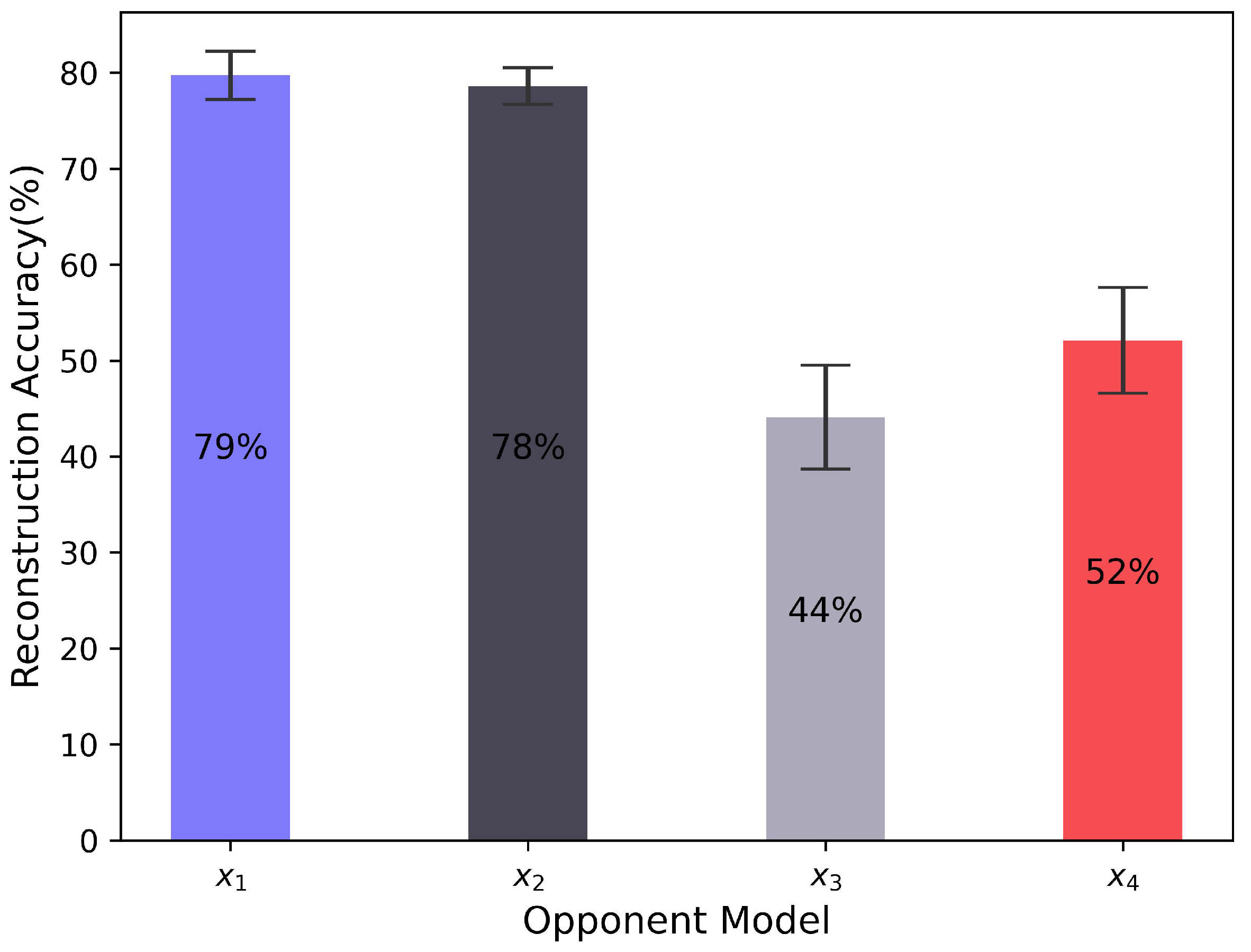
4.2. Results in the Offline Stage

In this section, we will evaluate the reconstruction accuracy of the opponent model and the distributions in the generated models. In the following experiments, we assume that the agent adopts the optimal response policy ${\pi }_i$ to play against the opponent policy ${\tau }_i$ and uses the opponent model $x_i$ to reconstruct the opponent’s actions.

Figure 4 illustrates the accuracy of the opponent model in reconstructing the opponent’s actions. We observe that both $x_1$ and $x_2$ can achieve an accuracy of approximately 80%, while $x_3$ and $x_4$ can only reach 44% and 52%. This is because ${\tau }_1$ and ${\tau }_2$ have fewer random actions to pursue the prey. In contrast, ${\tau }_3$ and ${\tau }_4$ have greater randomness, and they take all possible actions with a slight frequency difference, making VAE inaccurate in reconstructing the predators’ actions.

Figure 5 illustrates the performance model $P\left(U\left|\tau ,\pi \right.\right)$ (line 5 in Algorithm 1). Four opponent policies ${\left\{{\tau }_i\in \mathcal{T}\right\}}_{i=0}^{i=4}$ and four response policies ${\left\{{\pi }_i\in \mathrm{\Pi }\right\}}_{i=0}^{i=4}$ play against each other to fit sixteen Gaussian distributions. Each distribution reflects the corresponding episodic reward information. We observe that the optimal response policy receives the highest average episodic reward, all-around 10, with minor variance. In addition, the distribution is likely to be very similar to each other. For example, when the agent uses ${\pi }_1$, the distributions of interacting with ${\tau }_3$ and ${\tau }_4$ are almost the same. When the agent only uses the performance model to detect the opponent’s policy, such as BPR [39] and BPR+ [40], the high similarity of distributions may cause low detection accuracy.

Figure 6 illustrates the reconstruction accuracy model $\mathrm{\Omega }\left(W\left|\tau \right.,\pi ,x\right)$ (line 9 in Algorithm 1). It also consists of sixteen Gaussian distributions, like in the performance model P. Each distribution describes how accurately the corresponding opponent model x reconstructs the opponent’s actions. We observe that the optimal response policy has the highest accuracy, with ${\pi }_1$ and ${\pi }_2$ achieving an accuracy of around 80%, while ${\pi }_3$ and ${\pi }_4$ only reach approximately 50%. The difference between distributions in $\mathrm{\Omega }$ is more significant than that in P. For example, when the agent adopts ${\pi }_1$ to play against ${\tau }_3$ and ${\tau }_4$, the distributions in P are very similar, but they are much more different in $\mathrm{\Omega }$. In addition, $\mathrm{\Omega }$ is more suitable for situations where the opponent’s actions are available, and it can be jointly used with P during online detection.

Figure 7 shows the planning similarity model $\mathrm{\Theta }\left(Q\left|\tau ,\right.\pi ,x\right)$ (line 17 in Algorithm 1). We measure the similarity in terms of the mean square error between continuous observations. The smaller the error, the greater the similarity. We observe that the optimal response policy has the minimum mean squared error, with ${\pi }_1$ and ${\pi }_2$ reaching around 0. However, the minimum mean squared error for ${\pi }_3$ and ${\pi }_4$ is around 200 due to the lower accuracy of action reconstruction. In addition, $\mathrm{\Theta }$ is more suitable for situations where neither the opponent’s observations nor the actions are available, and it can also be used in combination with P during the online phase.

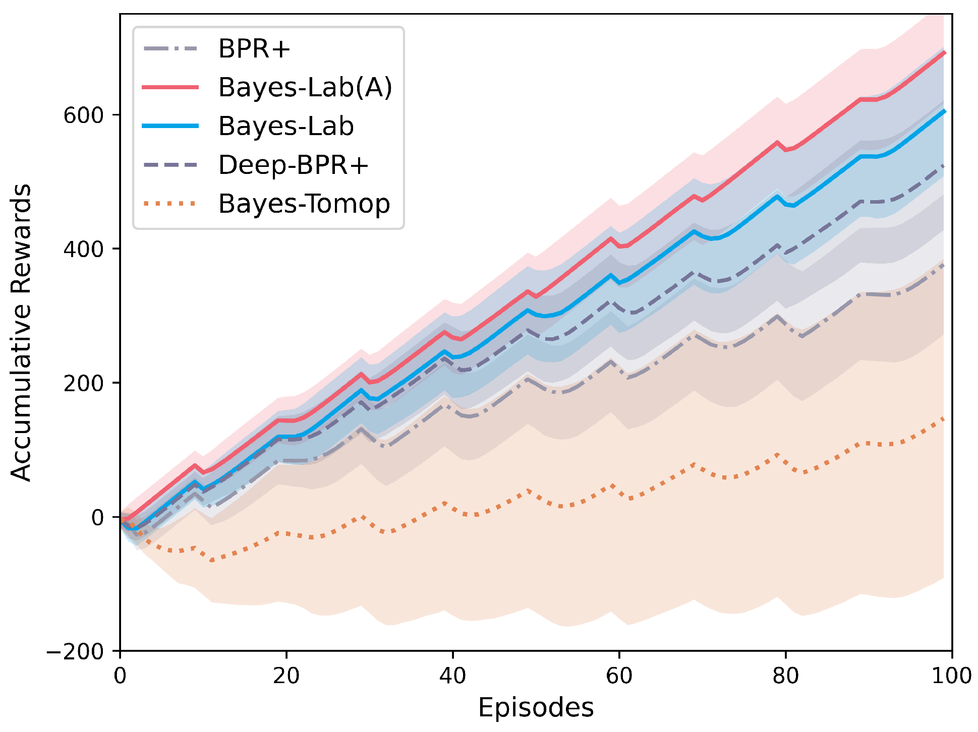
4.3. Results in Online Stage

In this section, we will evaluate the performance of Bayes-Lab by comparing it with the state-of-the-art algorithms, including BPR+ [40], Deep BPR+ [43], and Bayes-Tomop [44]. In the following experiments, we use Bayes-Lab(A) to represent the first detecting mode (line 10 in Algorithm 2), which combines $\mathrm{\Omega }$ with P to update $\beta \left(\tau \right)$, while using Bayes-Lab to define the second detecting mode (line 17 in Algorithm 2), which incorporates $\mathrm{\Theta }$ with P to detect the opponent’s type. In addition, we assume that the agent cannot obtain the opponent’s observations. We evaluated the performance of the proposed algorithm comprehensively through indicators such as episodic rewards, accumulated rewards, and detection accuracy. The following results were averaged over 500 runs to enable statistical analysis. There are 100 episodes in each run, and the opponents switch policies every 10 episodes. The order of policy switching is (${\tau }_2$, ${\tau }_3$, ${\tau }_1$, ${\tau }_3$, ${\tau }_4$, ${\tau }_1$, ${\tau }_4$, ${\tau }_1$, ${\tau }_3$, ${\tau }_1$). Each episode terminates after 100 time steps.

Figure 8 illustrates the episodic rewards for 100 episodes of interactions. The optimal reward will be around 10 within 100 time steps, as the agent receives a reward of 0.1 for each step without colliding with the opponents. We observe that the policy switch will lead to a rapid decrease in the reward, and the performance of the algorithms can be evaluated by observing how quickly the episodic rewards recover to 10. Bayes-Lab (A) recaptures the optimal reward most quickly during each policy switch. Bayes-Lab has a similar performance to Bayes-Lab (A) for the most part, but it has significantly lower rewards in episodes 50–60 and 70–80, where the policy switches from ${\tau }_4$ to ${\tau }_1$. By observing $\mathrm{\Omega }$ (Figure 6) and $\mathrm{\Theta }$ (Figure 7), we notice that the difference in the distributions in $\mathrm{\Omega }$ is more significant when the response policy is ${\pi }_4$. Therefore, $\mathrm{\Omega }$ is better suited to cope with the situation where the ${\tau }_4$ switches to ${\tau }_1$.

Moreover, Deep-BPR+ performs worse than Bayes-Lab (A) and Bayes-Lab because it overly depends on the opponent’s information and can only obtain the opponent’s behavior data within the agent’s vision range in our setting. BPR+ is slower to respond than Deep BPR+ because it detects the opponent based only on P (Figure 5). In other words, the distributions in P are relatively similar, resulting in poor performance for BPR+. Bayes-Tomop has the bottom performance of all algorithms as it takes additional steps to determine whether the opponent is using BPR, which is time-consuming.

Figure 9 illustrates the accumulative rewards for 100 episodes of interactions. We observe that the rewards decrease with each policy switch but increase again when detection and reuse are completed. Bayes-Lab (A) achieves the highest accumulative rewards because it detects and reuses the most quickly. Bayes-Lab has a lower performance than Bayes-Lab (A), but it is still better than the other algorithms because $\mathrm{\Theta }$ can compensate for the effects of the incomplete opponent information. Deep-BPR+ archives significantly higher rewards than BPR+, proving that detecting the opponent’s type by using its behaviors is more effective. Bayes-Tomop has the lowest rewards, demonstrating that it is inefficient in identifying whether the opponent is using BPR. Moreover, it assumes that the optimal rewards are consistent, but the agent may receive different optimal rewards in our setting, making detection more difficult.

Figure 10 shows the detection accuracy against non-stationary opponents. We observe that Bayes-Lab (A) and Bayes-Lab achieve relatively higher detection accuracies than other algorithms. We note that Bayes-Lab (A) and Bayes-Lab detect the opponent’s type only based on the agent’s observations. In contrast, Deep-BPR+ requires the opponent’s local information to achieve a high detection accuracy of 72%. BPR+ only achieves 65% detection accuracy by relying solely on reward signals. Bayes-Tomop has the lowest detection accuracy as it is hard to deal with opponents using random policies.

Figure 11 shows the switching interval’s effect on the algorithms’ performance. We design four switching intervals of 4, 8, 10, and 12, and we observe that the larger the switching interval, the higher the detection accuracy, with Bayes-Lab (A) and Bayes-Lab outperforming the other algorithms at all switching intervals. Specifically, when the switching interval is 12, the detection accuracy of all algorithms is relatively high, with Deep-BPR+ and BPR+ exceeding 70% and Bayes-Tomop exceeding 60%. When the switching interval changes from 12 to 8, there is a slight decrease in performance for all algorithms, and the degradation is relatively small for Bayes-Lab (A) and Bayes-Lab because they detect the opponent’s type most quickly. Most algorithms suffer a dramatic drop in performance when the switching interval changes from 8 to 4 because the opponent’s behaviors change rapidly. In this case, the gap between Bayes-Lab (A) and other algorithms increases obviously. In summary, the switching interval of the opponent policy has a crucial influence on detection accuracy. In other words, frequent switching strategies by opponents will lead to significant challenges to detection, while Bayes-Lab and Bayes-Lab (A) exhibit better performance in dealing with this problem due to $\mathrm{\Omega }$ and $\mathrm{\Theta }$.

Table 1. The effect of the switching interval on the accumulative rewards.

Algorithm	Switch Cycle 4	Switch Cycle 8	Switch Cycle 10	Switch Cycle 12
BPR+	−103.9 ± 73.6	190.9 ± 112.3	376.1 ± 104.5	563.4 ± 106.0
Deep-BPR+	−33.4 ± 89.4	326.5 ± 88.8	524.2 ± 96.8	728.8 ± 93.1
Bayes-Tomop	−171.6 ± 108.1	−16.1 ± 216.9	146.8 ± 237.9	302.7 ± 262.6
Bayes-Lab	23.9 ± 81.0	422.3 ± 82.5	604.3 ± 96.4	793.1 ± 90.5
Bayes-Lab (A)	131.8 ± 58.2	494.1 ± 74.8	691.6 ± 75.9	875.7 ± 74.6

shows the effect of the switching interval on the accumulative rewards. We observe that only Bayes-Lab (A) and Bayes-Lab have positive rewards when the switching interval is 4, and the other algorithms all have negative rewards, demonstrating that $\mathrm{\Omega }$ and $\mathrm{\Theta }$ effectively improve the performance against the opponent who switches policies frequently. Deep-BPR+ performs better than BPR+ and Bayes-Tomop, proving that it is essential for the agent to consider the opponent’s behaviors. The rewards improve significantly as the switching interval increases, showing that the longer the opponent’s policy remains fixed, the more accessible the agent can track the opponent. Bayes-Lab (A) and Bayes-Lab have similar performance, and their rewards far exceed that of BPR+ and Bayes-Tomop when the switching interval becomes 12. In summary, Bayes-Lab (A) and Bayes-Lab can adapt to a wide range of policy switching intervals without the opponent’s information.

5. Conclusions and Future Works

This paper focuses on accurate opponent policy detection and optimal response policy reuse in partially observable settings. The most significant contribution of the proposed algorithms, which include Bayes-Lab and Bayes-Lab (A), is that they can efficiently track the non-stationary opponents without their local information. Our model incorporates VAE into the BPR framework and follows the CTDE paradigm. It can reconstruct the opponent’s actions only based on its own local observations. Moreover, the reconstructed actions and episodic rewards are jointly used to update the belief about the opponent’s types. As a result, the agent can reuse the best response policies accurately. Extensive simulations in a predator–prey scenario with continuous observations and multiple opponents demonstrate that Bayes-Lab and Bayes-Lab (A) can adapt to a wide range of different policy switching intervals and achieve higher detection accuracy and accumulative rewards than other state-of-the-art algorithms. Many end applications that require quick online decisions may benefit from the proposed networks, such as human–computer interaction and service robots.

The main limitations of Bayes-Lab and Bayes-Lab (A) are as follows: First, we assume that the opponent’s behaviors significantly affect the agent’s local observations. However, the opponent’s behaviors may have little correlation to the agent’s local observations. In this case, it is difficult for the opponent model to learn the policy features of the opponent from the local observations. Second, we only consider the opponent switching policies at the end of an episode. However, the opponent may change more frequently, such as switching policies within an episode. Third, we assume that the opponent adopts its policy from a library that is fully known to the agent. However, the opponent may use a new strategy unknown to the agent. In future work, we would like to investigate how to build the model from different supervision signals rather than just depending on the opponent’s local information, and how to deal with opponents with abrupt policy changes, such as switching policies within an episode, is also worth investigating. Furthermore, we are also interested in accurately detecting the unknown opponent’s policy and learning a new optimal response policy by efficiently extracting available knowledge from the learned policies.

References

1. He, K.; Zhang, X.; Ren, S.; Sun, J. Deep residual learning for image recognition. In Proceedings of the IEEE Conference on Computer Vision and Pattern Recognition, Las Vegas, NV, USA, 26 June–1 July 2016; pp. 770–778. [Google Scholar]
2. Wang, J.; Chen, Y.; Hao, S.; Peng, X.; Hu, L. Deep learning for sensor-based activity recognition: A survey. Pattern Recognit. Lett. 2019, 119, 3–11. [Google Scholar] [CrossRef] [Green Version]
3. Kwon, H.; Lee, S. Ensemble transfer attack targeting text classification systems. Comput. Secur. 2022, 117, 102695. [Google Scholar] [CrossRef]
4. Kwon, H.; Lee, S. Textual Adversarial Training of Machine Learning Model for Resistance to Adversarial Examples. Secur. Commun. Netw. 2022, 2022, 4511510. [Google Scholar] [CrossRef]
5. Kwon, H.; Kim, Y. BlindNet backdoor: Attack on deep neural network using blind watermark. Multimed. Tools Appl. 2022, 81, 6217–6234. [Google Scholar] [CrossRef]
6. Lillicrap, T.P.; Hunt, J.J.; Pritzel, A.; Heess, N.; Erez, T.; Tassa, Y.; Silver, D.; Wierstra, D. Continuous control with deep reinforcement learning. arXiv 2015, arXiv:1509.02971. [Google Scholar]
7. Mnih, V.; Badia, A.P.; Mirza, M.; Graves, A.; Lillicrap, T.; Harley, T.; Silver, D.; Kavukcuoglu, K. Asynchronous methods for deep reinforcement learning. In Proceedings of the International Conference on Machine Learning, New York, NY, USA, 20–22 June 2016; pp. 1928–1937. [Google Scholar]
8. Van Hasselt, H.; Guez, A.; Silver, D. Deep reinforcement learning with double q-learning. In Proceedings of the AAAI Conference on Artificial Intelligence, Phoenix, AZ, USA, 12–17 February 2016; Volume 30. [Google Scholar]
9. Silver, D.; Huang, A.; Maddison, C.J.; Guez, A.; Sifre, L.; Van Den Driessche, G.; Schrittwieser, J.; Antonoglou, I.; Panneershelvam, V.; Lanctot, M.; et al. Mastering the game of Go with deep neural networks and tree search. Nature 2016, 529, 484–489. [Google Scholar] [CrossRef]
10. Mnih, V.; Kavukcuoglu, K.; Silver, D.; Rusu, A.A.; Veness, J.; Bellemare, M.G.; Graves, A.; Riedmiller, M.; Fidjeland, A.K.; Ostrovski, G.; et al. Human-level control through deep reinforcement learning. Nature 2015, 518, 529–533. [Google Scholar] [CrossRef]
11. Gu, S.; Holly, E.; Lillicrap, T.; Levine, S. Deep reinforcement learning for robotic manipulation with asynchronous off-policy updates. In Proceedings of the 2017 IEEE International Conference on Robotics and Automation (ICRA), Singapore, 29 May–3 June 2017; pp. 3389–3396. [Google Scholar]
12. Tai, L.; Paolo, G.; Liu, M. Virtual-to-real deep reinforcement learning: Continuous control of mobile robots for mapless navigation. In Proceedings of the 2017 IEEE/RSJ International Conference on Intelligent Robots and Systems (IROS), Vancouver, BC, Canada, 24–28 September 2017; pp. 31–36. [Google Scholar]
13. Zhang, F.; Leitner, J.; Milford, M.; Upcroft, B.; Corke, P. Towards vision-based deep reinforcement learning for robotic motion control. arXiv 2015, arXiv:1511.03791. [Google Scholar]
14. Barzegar, A.; Lee, D.J. Deep Reinforcement Learning-Based Adaptive Controller for Trajectory Tracking and Altitude Control of an Aerial Robot. Appl. Sci. 2022, 12, 4764. [Google Scholar] [CrossRef]
15. Sallab, A.E.; Abdou, M.; Perot, E.; Yogamani, S. Deep reinforcement learning framework for autonomous driving. Electron. Imaging 2017, 2017, 70–76. [Google Scholar] [CrossRef] [Green Version]
16. Kiran, B.R.; Sobh, I.; Talpaert, V.; Mannion, P.; Al Sallab, A.A.; Yogamani, S.; Pérez, P. Deep reinforcement learning for autonomous driving: A survey. IEEE Trans. Intell. Transp. Syst. 2021, 23, 4909–4926. [Google Scholar] [CrossRef]
17. Chang, C.C.; Tsai, J.; Lin, J.H.; Ooi, Y.M. Autonomous Driving Control Using the DDPG and RDPG Algorithms. Appl. Sci. 2021, 11, 10659. [Google Scholar] [CrossRef]
18. Zhao, W.; Meng, Z.; Wang, K.; Zhang, J.; Lu, S. Hierarchical Active Tracking Control for UAVs via Deep Reinforcement Learning. Appl. Sci. 2021, 11, 10595. [Google Scholar] [CrossRef]
19. Wooldridge, M. An Introduction to Multiagent Systems; John Wiley & Sons: Hoboken, NJ, USA, 2009. [Google Scholar]
20. Nguyen, T.T.; Nguyen, N.D.; Nahavandi, S. Deep reinforcement learning for multiagent systems: A review of challenges, solutions, and applications. IEEE Trans. Cybern. 2020, 50, 3826–3839. [Google Scholar] [CrossRef] [Green Version]
21. Conitzer, V.; Sandholm, T. AWESOME: A general multiagent learning algorithm that converges in self-play and learns a best response against stationary opponents. Mach. Learn. 2007, 67, 23–43. [Google Scholar] [CrossRef] [Green Version]
22. Chen, H.; Liu, Q.; Huang, J.; Fu, K. Efficiently tracking multi-strategic opponents: A context-aware Bayesian policy reuse approach. Appl. Soft Comput. 2022, 121, 108715. [Google Scholar] [CrossRef]
23. Chen, H.; Liu, Q.; Fu, K.; Huang, J.; Wang, C.; Gong, J. Accurate policy detection and efficient knowledge reuse against multi-strategic opponents. Knowl.-Based Syst. 2022, 242, 108404. [Google Scholar] [CrossRef]
24. Sutton, R.S.; Barto, A.G. Reinforcement Learning: An Introduction; MIT Press: Cambridge, MA, USA, 2018. [Google Scholar]
25. Hernandez-Leal, P.; Kaisers, M. Towards a fast detection of opponents in repeated stochastic games. In International Conference on Autonomous Agents and Multiagent Systems; Springer: Berlin/Heidelberg, Germany, 2017; pp. 239–257. [Google Scholar]
26. Hernandez-Leal, P.; Kaisers, M.; Baarslag, T.; de Cote, E.M. A survey of learning in multiagent environments: Dealing with non-stationarity. arXiv 2017, arXiv:1707.09183. [Google Scholar]
27. Rabinowitz, N.; Perbet, F.; Song, F.; Zhang, C.; Eslami, S.A.; Botvinick, M. Machine theory of mind. In Proceedings of the International Conference on Machine Learning, Stockholm, Sweden, 10–15 July 2018; pp. 4218–4227. [Google Scholar]
28. Papoudakis, G.; Christianos, F.; Rahman, A.; Albrecht, S.V. Dealing with non-stationarity in multi-agent deep reinforcement learning. arXiv 2019, arXiv:1906.04737. [Google Scholar]
29. He, H.; Boyd-Graber, J.; Kwok, K.; Daumé, H., III. Opponent modeling in deep reinforcement learning. In Proceedings of the International Conference on Machine Learning, New York, NY, USA, 20–22 June 2016; pp. 1804–1813. [Google Scholar]
30. Albrecht, S.V.; Stone, P. Autonomous agents modelling other agents: A comprehensive survey and open problems. Artif. Intell. 2018, 258, 66–95. [Google Scholar] [CrossRef] [Green Version]
31. Grover, A.; Al-Shedivat, M.; Gupta, J.; Burda, Y.; Edwards, H. Learning policy representations in multiagent systems. In Proceedings of the International Conference on Machine Learning, Stockholm, Sweden, 10–15 July 2018; pp. 1802–1811. [Google Scholar]
32. Tacchetti, A.; Song, H.F.; Mediano, P.A.; Zambaldi, V.; Rabinowitz, N.C.; Graepel, T.; Botvinick, M.; Battaglia, P.W. Relational forward models for multi-agent learning. arXiv 2018, arXiv:1809.11044. [Google Scholar]
33. Hernandez-Leal, P.; Kartal, B.; Taylor, M.E. A survey and critique of multiagent deep reinforcement learning. Auton. Agents Multi-Agent Syst. 2019, 33, 750–797. [Google Scholar] [CrossRef] [Green Version]
34. Raileanu, R.; Denton, E.; Szlam, A.; Fergus, R. Modeling others using oneself in multi-agent reinforcement learning. In Proceedings of the International Conference on Machine Learning, Stockholm, Sweden, 10–15 July 2018; pp. 4257–4266. [Google Scholar]
35. Mnih, V.; Kavukcuoglu, K.; Silver, D.; Graves, A.; Antonoglou, I.; Wierstra, D.; Riedmiller, M. Playing atari with deep reinforcement learning. arXiv 2013, arXiv:1312.5602. [Google Scholar]
36. Hong, Z.W.; Su, S.Y.; Shann, T.Y.; Chang, Y.H.; Lee, C.Y. A deep policy inference q-network for multi-agent systems. arXiv 2017, arXiv:1712.07893. [Google Scholar]
37. Papoudakis, G.; Christianos, F.; Albrecht, S. Agent Modelling under Partial Observability for Deep Reinforcement Learning. Adv. Neural Inf. Process. Syst. 2021, 34, 19210–19222. [Google Scholar]
38. Kingma, D.P.; Welling, M. Auto-encoding variational bayes. arXiv 2013, arXiv:1312.6114. [Google Scholar]
39. Rosman, B.; Hawasly, M.; Ramamoorthy, S. Bayesian policy reuse. Mach. Learn. 2016, 104, 99–127. [Google Scholar] [CrossRef] [Green Version]
40. Hernandez-Leal, P.; Taylor, M.E.; Rosman, B.; Sucar, L.E.; De Cote, E.M. Identifying and tracking switching, non-stationary opponents: A Bayesian approach. In Proceedings of the Workshops at the Thirtieth AAAI Conference on Artificial Intelligence, Phoenix, AZ, USA, 12–13 February 2016. [Google Scholar]
41. Harsanyi, J.C. Games with incomplete information played by “Bayesian” players, I–III Part I. The basic model. Manag. Sci. 1967, 14, 159–182. [Google Scholar] [CrossRef]
42. Crandall, J.W. Just add Pepper: Extending learning algorithms for repeated matrix games to repeated markov games. In Proceedings of the 11th International Conference on Autonomous Agents and Multiagent Systems, Valencia, Spain, 4–8 June 2012; Volume 1, pp. 399–406. [Google Scholar]
43. Zheng, Y.; Meng, Z.; Hao, J.; Zhang, Z.; Yang, T.; Fan, C. A deep bayesian policy reuse approach against non-stationary agents. Adv. Neural Inf. Process. Syst. 2018, 31, 962–972. [Google Scholar]
44. Yang, T.; Meng, Z.; Hao, J.; Zhang, C.; Zheng, Y.; Zheng, Z. Towards efficient detection and optimal response against sophisticated opponents. arXiv 2018, arXiv:1809.04240. [Google Scholar]
45. Papoudakis, G.; Christianos, F.; Albrecht, S.V. Local Information Opponent Modelling Using Variational Autoencoders. arXiv 2020, arXiv:2006.09447. [Google Scholar]
46. Bellman, R. A Markovian decision process. J. Math. Mech. 1957, 6, 679–684. [Google Scholar] [CrossRef]
47. Zacharaki, A.; Kostavelis, I.; Dokas, I. Decision Making with STPA through Markov Decision Process, a Theoretic Framework for Safe Human-Robot Collaboration. Appl. Sci. 2021, 11, 5212. [Google Scholar] [CrossRef]
48. Doersch, C. Tutorial on variational autoencoders. arXiv 2016, arXiv:1606.05908. [Google Scholar]
49. Hinton, G.E.; Salakhutdinov, R.R. Reducing the dimensionality of data with neural networks. Science 2006, 313, 504–507. [Google Scholar] [CrossRef] [PubMed] [Green Version]
50. Bottou, L. Stochastic gradient descent tricks. In Neural Networks: Tricks of the Trade; Springer: Berlin/Heidelberg, Germany, 2012; pp. 421–436. [Google Scholar]
51. Yan, X.; Yang, J.; Sohn, K.; Lee, H. Attribute2image: Conditional image generation from visual attributes. In Proceedings of the European Conference on Computer Vision, Munich, Germany, 8–14 September 2016; pp. 776–791. [Google Scholar]
52. Ha, D.; Schmidhuber, J. Recurrent world models facilitate policy evolution. In Proceedings of the Advances in Neural Information Processing Systems 31, Montréal, QC, Canada, 3–8 December 2018. [Google Scholar]
53. Igl, M.; Zintgraf, L.; Le, T.A.; Wood, F.; Whiteson, S. Deep variational reinforcement learning for POMDPs. In Proceedings of the International Conference on Machine Learning, Stockholm, Sweden, 10–15 July 2018; pp. 2117–2126. [Google Scholar]
54. Higgins, I.; Matthey, L.; Pal, A.; Burgess, C.; Glorot, X.; Botvinick, M.; Mohamed, S.; Lerchner, A. Beta-vae: Learning basic visual concepts with a constrained variational framework. In Proceedings of the International Conference on Learning Representations, Toulon, France, 24–26 April 2017. [Google Scholar]
55. Gretton, A.; Borgwardt, K.; Rasch, M.; Schölkopf, B.; Smola, A. A kernel method for the two-sample-problem. arXiv 2006, arXiv:0805.2368. [Google Scholar]
56. Zhao, S.; Song, J.; Ermon, S. Infovae: Information maximizing variational autoencoders. arXiv 2017, arXiv:1706.02262. [Google Scholar]
57. Stone, P.; Veloso, M. Multiagent systems: A survey from a machine learning perspective. Auton. Robot. 2000, 8, 345–383. [Google Scholar] [CrossRef]
58. Böhmer, W.; Kurin, V.; Whiteson, S. Deep coordination graphs. In Proceedings of the International Conference on Machine Learning, Virtual, 13–18 July 2020; pp. 980–991. [Google Scholar]
59. Lowe, R.; Wu, Y.I.; Tamar, A.; Harb, J.; Abbeel, O.P.; Mordatch, I. Multi-agent actor-critic for mixed cooperative-competitive environments. arXiv 2017, arXiv:1706.0227530. [Google Scholar]
60. Son, K.; Kim, D.; Kang, W.J.; Hostallero, D.E.; Yi, Y. Qtran: Learning to factorize with transformation for cooperative multi-agent reinforcement learning. In Proceedings of the International Conference on Machine Learning, Long Beach, CA, USA, 9–15 June 2019; pp. 5887–5896. [Google Scholar]
Figure 1. An overview of Bayes-Lab.
Applsci 12 06953 g001
Figure 2. Diagram of offline learning architecture.
Applsci 12 06953 g002
Figure 3. Predator–Prey: an adversarial multi-agent environment used in our evaluation.
Applsci 12 06953 g003
Figure 4. The accuracy of the opponent model in reconstructing the opponent’s actions.
Applsci 12 06953 g004
Figure 5. The performance model P.
Applsci 12 06953 g005
Figure 6. The reconstruction accuracy model Ω .
Applsci 12 06953 g006
Figure 7. The planning similarity model Θ .
Applsci 12 06953 g007
Figure 8. The episodic rewards for 100 episodes of interactions.
Applsci 12 06953 g008
Figure 9. The accumulative rewards for 100 episodes of interactions.
Applsci 12 06953 g009
Figure 10. The detection accuracy against non-stationary opponents.
Applsci 12 06953 g010
Figure 11. The effect of the switching interval on the detection accuracy.
Applsci 12 06953 g011